


Introduction and motivation
This review represents the Southern Ocean community’s satellite needs for the coming decade. It is designed to stand as an important strategy paper that provides the rationale and information required for future strategic planning and investment.
The Southern Ocean (defined herein as south of 30°S, although the expertise of those who replied and commented is largely restricted to higher latitude oceans, which limits some of the topics discussed in this paper) has a profound influence on the global ocean circulation and the Earth’s climate. It uniquely connects the Earth’s ocean basins and plays a key role in global overturning circulation, thereby regulating the capacity of the ocean to store and transport heat, carbon and other properties that influence climate and global biogeochemical cycles. Global climate and sea level are influenced strongly by ocean–cryosphere interactions in the Southern Ocean. Changes in the extent or volume of sea ice result in changes in the Earth’s albedo, water mass formation rates and air–sea gas exchange rates, and effects on marine organisms from microbes to whales (see Rintoul et al. Reference Rintoul, Sparrow, Meredith, Wadley, Speer, Hofmann, Summerhayes, Urban and Bellerby2012 for more detailed information on the importance of the Southern Ocean in the global climate and biogeochemical system).
Given the central role that the Southern Ocean plays in the global climate system, any changes in the region will have global consequences. The Southern Ocean Observing System (SOOS) Initial Science and Implementation Strategy (Rintoul et al. Reference Rintoul, Sparrow, Meredith, Wadley, Speer, Hofmann, Summerhayes, Urban and Bellerby2012) provides an overview of how an effective observing system could be built for the Southern Ocean and highlights the importance of remote sensing in providing fundamental observational data of surface and near-surface properties in this remote region, where in situ observations will probably always be sparse and hard to obtain. A valuable review of recent developments and upcoming plans in satellite oceanography was recently published by Le Traon et al. (Reference Le Traon, Antoine, Bentamy, Bonekamp, Breivik, Chapron, Corlett, Dibarboure, DiGiacomo, Donlon, Faugere, Font, Girard-Ardhuin, Gohin, Johannessen, Kamachi, Lagerloef, Lambin, Larnicol, Le Borgne, Leuliette, Lindstrom, Martin, Maturi, Miller, Mingsen, Morrow, Reul, Rio, Roquet, Santoleri and Wilkin2015), demonstrating progress in the discipline at the time this paper was being compiled and written. In addition, for a review of open access data, including various satellites and their lifetimes, see Pope et al. (Reference Pope, Rees, Fox and Fleming2014). Nevertheless, remote sensing of the Southern Ocean is not without significant challenges and much work is needed to enhance cross-calibration and independent validation with in situ data, improve algorithms and geophysical corrections, ensure continuity of time series, and drive development of better sensor technology and global climate prediction models.
There are many similarities between Arctic and Antarctic/Southern Ocean remote sensing, but different geographical settings introduce unique challenges to each. Although differences exist in the validity and accuracy of specific algorithms and corrections between the Northern and Southern Hemisphere polar oceans, data requirements are largely the same. Yet, some missions focus acquisitions and data analysis predominantly on Arctic objectives, owing to the strong scientific, commercial and operational rationale, as well as the national priorities of the key data providers. Sentinel observation requirements, for example, are currently justified by Copernicus services and national requirements relevant to EU users in specific geographical zones. The Copernicus programme and the Sentinels are planned to address many community requests (e.g. data access, higher revisit frequency, standard data formats, continuity of crucial datasets, etc.), and some will be relevant for polar research and the Southern Ocean (Malenovský et al. Reference Malenovský, Rott, Cihlar, Schaepman, García-Santos, Fernandes and Berger2012). However, whilst the satellites are cited as providing routine global coverage, the data acquisition strategies and resulting datasets are not characterized by ‘all the time, everywhere’ (and admittedly cannot fully be so, because of limited duty cycles per orbit). A clear example of this is that Sentinel-2 will be mostly inactive south of the southern tip of Chile (dependent on particular requests and subject to special approval), raising the question about the means to obtain optical coverage of the Southern Ocean or Antarctic ice shelves. Today there are no operational high priority Copernicus user service requirements to drive these data acquisitions. Addressing this oversight is crucial to ensure a well-balanced polar science data collection strategy from the Copernicus Sentinels (Aschbacher & Milagro-Pérez Reference Aschbacher and Milagro-Pérez2012, Donlon et al. Reference Donlon, Berruti, Buongiorno, Ferreira, Femenias, Frerick, Goryl, Klein, Laur, Mavrocordatos, Nieke, Rebhan, Seitz, Stroede and Sciarra2012, Drusch et al. Reference Drusch, Del Bello, Carlier, Colin, Fernandez, Gascon, Hoersch, Isola, Laberinti, Martimort, Meygret, Spoto, Sy, Marchese and Bargellini2012, Torres et al. Reference Torres, Snoeji, Geudtner, Bibby, Davidson, Attema, Potin, Rommen, Floury, Brown, Traver, Deghaye, Duesmann, Rosich, Miranda, Bruno, L'Abbate, Croci, Pietropaolo, Huchler and Rostan2012). Similarly, RADARSAT-2 (http://www.asc-csa.gc.ca/eng/satellites/radarsat2/) and the RADARSAT Constellation (http://www.asc-csa.gc.ca/eng/satellites/radarsat/) missions are focused on the Arctic, owing predominantly to the commercial customer base.
In order to address these and other disparities in polar remote sensing, and to articulate the satellite needs specific to the Southern Ocean, SOOS (an initiative of the Scientific Committee on Oceanic Research (SCOR) and the Scientific Committee on Antarctic Research (SCAR)) and the World Climate Research Programme’s Climate and Cryosphere project (WCRP CliC) sanctioned this community review to offer a consolidated user voice. It provides an overview of satellite data requirements for the Southern Ocean (including scientific, commercial and operational rationales) towards achieving the objective of ensuring continuation and enhancement of Southern Ocean satellite data. This review also features the results of a survey tailored specifically to ensure community input. Its scope includes satellite data requirements for the open and sea ice-covered portions of the Southern Ocean, including the coastal and fast ice zones, and oceanic connections to the continent through ice shelves. Terrestrial data requirements are largely outside the scope of this report. This review should be considered alongside the recommendations of parallel efforts, including the SCAR Horizon Scan (Kennicutt et al. Reference Kennicutt, Chown, Cassano, Liggett, Massom, Peck, Rintoul, Storey, Vaughan, Wilson and Sutherland2014), the Year of Polar Prediction (Goessling et al. Reference Goessling, Jung, Klebe, Baeseman, Bauer, Chen, Chevallier, Dole, Gordon, Ruti, Bradley, Bromwich, Casati, Chechin, Day, Massonnet, Mills, Renfrew, Smith and Tatusko2016), the outcomes of a European Space Agency (ESA) cryosphere workshop (Fernández-Prieto et al. Reference Fernández-Prieto, Hogg, Bamber, Baeseman, Drinkwater, Ryabinin, Steffen, Dierking, Duguay, Gerland, Giles, Haas, Heim, Howell, Joughin, Kaleschke, Kern, Laxon, Macelloni, Painter, Paul, Payne, Pedersen, Pulliainen, Rack, Rignot, Rott, Scambos, Schrama, Shepherd, Strozzi, van den Broeke, Velicogna and Zwally2013) and an ESA-CliC workshop focussing on Arctic satellite data needs (Baeseman & Fernández-Prieto Reference Baseman and Fernández Prieto2015).
Importantly, this review also links the observational priorities defined herein to the global effort to identify essential variables for climate and ocean, specifically Essential Climate Variables (ECVs, Bojinski et al. Reference Bojinski, Verstraete, Peterson, Richter, Simmons and Zemp2014) and Essential Ocean Variables (EOVs). In particular, this review highlights connections with EOVs and ECVs of the Ocean Observations Panel for Climate (OOPC) and the World Meteorological Organization Global Climate Observing System (WMO GCOS), the ECVs defined by the ESA Climate Change Initiative (CCI) and SOOS EOVs. While there is currently no consistency in the definition of an ECV or EOV between communities, this report follows the SOOS definition whereby an EOV has a unit of measurement. Regardless, the recognition of these variables as ‘essential’ indicates global agreement in the priority for their inclusion in observing systems.
Community consultation
Between 12 March and 26 June 2014, the survey introduced above was open to input from members of the Southern Ocean community, spanning a wide range of research and operational disciplines and goals. Although the survey was open to comments regarding the mid-latitudes through to polar ocean considerations, the expertise of most of those who responded centred largely on Antarctic coastal waters and regions with ice. The survey received 59 unique responses from 19 countries worldwide (Fig. 1). Full survey questions are available in the supplemental material (found at http://dx.doi.org/10.1017/S0954102016000390) and full survey responses (except personal information) are available as a separate supplement (Pope et al. Reference Pope, Wagner, Johnson, Baeseman and Newman2015).
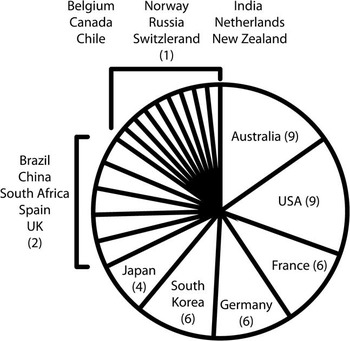
Fig. 1 Nationalities of survey respondents.
Most survey respondents were researchers, while only two identified primarily as operational remote sensing users (‘Icebreaker Science Liaison’ and ‘national Antarctic programme operations involving ships, aircraft and ground activity’). Scientific expertise of respondents included sea ice research (13), oceanography (11), marine biology and ecology (8), glaciology/permafrost/snow science (6), sea level change (5), ocean colour remote sensing (5), climate science (5), ocean winds (2), data collection and management (2), numerical weather prediction (1), atmospheric chemistry (1) and geomagnetism (1); note, there is some overlap in areas of expertise. For clarity in discussing contributions from this group, information gained from the survey will be termed as coming from ‘respondents’.
To ensure that we accurately captured the Southern Ocean community response and to broaden feedback in key disciplines and user groups, we specifically contacted members of the community and solicited their input. In particular, there were minimal or no survey respondents who provided feedback on sea surface salinity, surface winds or atmospheric parameters, so nine experts in these specialties were consulted to supplement a literature review in this regard. These experts will be referred to as ‘contributors’ to clarify their contributions. Finally, a draft version of the review was made available for public consultation via major Antarctic and Southern Ocean community listservs (e.g. Cryolist) and newsletters (e.g. SCAR, SOOS, International Ice Charting Working Group (IICWG) and CliC); over 25 respondents from a range of specialties commented in that final stage of review development, referred to as ‘commenters’. While respondents are anonymous, see the Acknowledgements section for all contributors and commenters.
Sea ice
Importance of sea ice observations
Sea ice is an important part of the cryosphere, and it is ice made of saline water floating on the polar oceans. It changes significantly on seasonal and annual timescales, and acts as a considerable reflector of incoming solar radiation, which regulates local and global energy balances between the atmosphere and the underlying sea surface (Perovich Reference Perovich2011). Sea ice growth and formation plays a role in air–ice–ocean heat, gas and freshwater fluxes on seasonal timescales. Approximately 7% of the Earth’s surface or 10% of the ocean surface is covered by sea ice at some point within the year and thus plays a critical role with other parameters in the Earth’s global system (Parkinson Reference Parkinson2014). As global temperatures are increasing at rapid rates, sea ice response may also be a sensitive indicator of our changing climate (Massom & Stammerjohn Reference Massom and Stammerjohn2010, Landrum et al. Reference Landrum, Holland, Schneider and Hunke2012). Sea ice cover around the Antarctic varies strongly by region and season due to its dynamic growth and retreat, especially in the Ross, Bellingshausen-Amundsen and Weddell seas (Cavalieri & Parkinson Reference Cavalieri and Parkinson2008, Parkinson & Cavalieri Reference Parkinson and Cavalieri2012). Due to the high level of turbulence in the Southern Ocean, Antarctic sea ice contains largely frazil, pancake and first-year ice types. It is very rare for calm conditions and lack of swell waves to prevail long enough for large expanses of undeformed nilas and grey-white ice to form (Massom Reference Massom2009). Antarctic sea ice has also demonstrated a strong response to winds and atmospheric variability, and is potentially influenced by large-scale climate variability patterns, such as the El Niño Southern Oscillation and Southern Annular Mode (SAM) (Marshall Reference Marshall2003, Holland & Kwok Reference Holland and Kwok2012, Maksym et al. Reference Maksym, Stammerjohn, Ackley and Massom2012, Raphael & Hobbs Reference Raphael and Hobbs2014). Although overall positive trends have been observed with regards to the sea ice extent, there continues to be strong patterns of regional variability where some regions show an increase and others are decreasing (Meier & Markus Reference Meier and Markus2015).
Although sea ice is often viewed as a single component of the cryosphere, it is actually a complex material characterized by a number of different parameters (i.e. thickness, sea ice area fraction, ice type, ice drift and snow cover on sea ice), all of which affect how accurately we can measure sea ice features. To improve the accuracy in monitoring sea ice conditions, it is particularly important for observational scientists to understand the types of in situ data that can be used in validation, both for long-term monitoring products where the datasets are acquired over a long time period, and for tactical products used for navigational safety where there is an additional focus on timely and reliable delivery.
Operational monitoring includes providing support to fishing vessels, icebreakers, other cargo ships transporting supplies to scientific bases on the Antarctic continent, tourist ships and military transits. As operations, industry and tourist vessels continue to traverse through sea ice-infested areas, it is important to have accurate knowledge of sea ice conditions so that non-ice strengthened ships have ample time to avoid or navigate safely and efficiently through these areas. For operations, Antarctica is continuously observed with the use of multiple data sources to produce sea ice charts that provide large-scale and global coverage year-round (e.g.https://nsidc.org/noaa/iicwg).
The following sea ice parameters described in this review are critical to sea ice as an ECV and the SOOS EOVs, as described in the SOOS Science Theme 5: the future of Antarctic sea ice (Rintoul et al. Reference Rintoul, Sparrow, Meredith, Wadley, Speer, Hofmann, Summerhayes, Urban and Bellerby2012). Additionally, monitoring changes in sea ice is particularly important to SOOS due to the multi-faceted relationship of sea ice and the freshwater balance, albedo, oceanic air–sea CO2 flux and biological activity in the Southern Ocean.
Current status of sea ice observations
Monitoring sea ice in the Southern Ocean uses data from optical (visible) and infrared radiation, imaging sensors (passive microwave and synthetic aperture radar (SAR)), non-imaging radar sensors (scatterometer) and nadir-ranging sensors (laser and radar altimeters). Although optical imagery is used when there are clear cloud conditions, imaging and nadir-ranging sensors can collect data through cloud cover and during the winter when there is little to no solar illumination (Carsey Reference Carsey1992, Lubin & Massom Reference Lubin and Massom2006). Detailed descriptions of fundamental concepts and principles of these sensors on sea ice can be found in Carsey (Reference Carsey1992), Lubin & Massom (Reference Lubin and Massom2006), Massom (Reference Massom2009), Weeks (Reference Weeks2010) and Tedesco (Reference Tedesco2015).
Sea ice concentration, also known as sea ice area fraction, is measured indirectly by the level of emissivity, or reflectivity, seen by a sensor (Lubin & Massom Reference Lubin and Massom2006). Since the 1970s, passive microwave data have been used to compute the Southern Ocean sea ice area fraction (Comiso et al. Reference Comiso, Cavalieri, Parkinson and Gloersen1997, Comiso & Nishio Reference Comiso and Nishio2008, Parkinson & Cavalieri Reference Parkinson and Cavalieri2012) and more or less consistent, continuous sea ice records suitable for time series analysis exist after multifrequency sensors were introduced in 1979 (Peng et al. Reference Peng, Meier, Scott and Savoie2013, Eastwood et al. Reference Eastwood, Jenssen, Lavergne, Sørensen and Tonboe2015, Ivanova et al. Reference Ivanova, Pedersen, Tonboe, Kern, Heygster, Lavergne, Sørensen, Saldo, Dybkjær, Brucker and Shokr2015). Survey respondents referred to passive microwave data as being the main source for a comprehensive climate record because of its high temporal resolution and longest continuous data record. Also, when combining several algorithms for sea ice concentration, it was shown that a combination of algorithms for the 19 GHz and 37 GHz channels can provide reliable global sea ice concentration data that extends from 1978 to the present (Ivanova et al. Reference Ivanova, Pedersen, Tonboe, Kern, Heygster, Lavergne, Sørensen, Saldo, Dybkjær, Brucker and Shokr2015).
Several types of active radar satellite-derived data include: SAR, scatterometry and radar altimetry. Some advantages of using SAR data are that it provides higher spatial resolution images (which allows the user to detect smaller features such as leads, floes, ridges, polynyas) and that it can be used to augment other high spatial resolution satellite products, such as optical or infrared when there is cloud cover over a particular area (Lubin & Massom Reference Lubin and Massom2006). Such detailed images also have the ability to develop more realistic models of the rheology of sea ice and sea ice drift (Carsey et al. Reference Carsey, Harding and Wales1998, Linow et al. Reference Linow, Hollands and Dierking2015). Additionally, the lack of pixel mixing allows for details over large areas to be discernible, which can be particularly important at the ice edge where the sea ice can be dispersed (Carsey et al. Reference Carsey, Harding and Wales1998, Lubin & Massom Reference Lubin and Massom2006). The disadvantages of SAR are that it does not provide synoptic coverage, there are greater data archives and volumes with passive microwave, and the data processing is more complicated because radiometric corrections should be applied to resolve incidence angles for different backscatter magnitudes across varying incidence angles (Lubin & Massom Reference Lubin and Massom2006, Moen et al. Reference Moen, Anfinsen, Dougleris, Renner and Gerland2015).
Before presenting information on how sea ice parameters are monitored, it is necessary to describe the impact of snow cover on sea ice. Snow cover on sea ice is an important parameter because it affects the accuracy of sea ice thickness measurements and affects microwave properties when identifying sea ice area fraction. According to respondents and commenters, commonly used snow depth products derived from passive microwave data are the Advanced Microwave Scanning Radiometer - Earth Observing System (AMSR-E; and later AMSR-2) products that were developed by NASA and hosted at the National Snow and Ice Data Center (NSIDC) (Comiso et al. Reference Comiso, Cavalieri and Markus2003) following initial research using the Special Sensor Microwave Imager (SSM/I) 19 and 37 GHz vertical polarization channels (Markus & Cavalieri Reference Markus and Cavalieri1998), and the snow depth product developed at the University of Bremen (Frost et al. Reference Frost, Heygster and Kern2014). All three products are used, but based on the survey consultation, the AMSR-E (Comiso et al. Reference Comiso, Cavalieri and Markus2003) and University of Bremen (Frost et al. Reference Frost, Heygster and Kern2014) products are used the most (Zwally et al. Reference Zwally, Yi, Kwok and Zhao2008, Kurtz & Markus Reference Kurtz and Markus2012, Xie et al. Reference Xie, Tekli, Ackley, Yi and Zwally2013, Kern & Spreen Reference Kern and Spreen2015, Schwegmann et al. Reference Schwegmann, Rinne, Ricker, Hendricks and Helm2016).
Survey respondents noted that much of the ice thickness data available has been retrieved from the Arctic. The Antarctic is more difficult, especially for altimeters, because there is ambiguity in the relationship between freeboard and total thickness because of flooded snow and snow–ice formation. From the survey and community feedback, common mechanisms to measure sea ice thickness are spaceborne laser altimetry (ICESat) (Zwally et al. Reference Zwally, Yi, Kwok and Zhao2008, Kurtz & Markus Reference Kurtz and Markus2012, Ozsoy-Cicek et al. Reference Ozsoy-Cicek, Ackley, Xie, Yi and Zwally2013, Xie et al. Reference Xie, Tekli, Ackley, Yi and Zwally2013, Kern & Spreen Reference Kern and Spreen2015) and radar (Cryosat-2) (Price et al. Reference Price, Beckers, Ricker, Kurtz, Rack, Haas, Helm, Hendricks, Leonard and Langhorne2015, Schwegmann et al. Reference Schwegmann, Rinne, Ricker, Hendricks and Helm2016). In comparison with in situ measurements (e.g. autonomous underwater vehicle (AUV), upward looking sonar (ULS), electromagnetic (EM)-data, airborne altimetry), these sensors have produced robust estimates of Antarctic sea ice thickness, although they are still being validated (Zwally et al. Reference Zwally, Yi, Kwok and Zhao2008, Markus et al. Reference Markus, Massom, Worby, Lytle, Kurtz and Maksym2011, Kurtz & Markus Reference Kurtz and Markus2012, Kurtz et al. Reference Kurtz, Galin and Studinger2014, Price et al. Reference Price, Beckers, Ricker, Kurtz, Rack, Haas, Helm, Hendricks, Leonard and Langhorne2015). Radar altimeters have the capability to penetrate through the snow cover and return off the snow–ice, snow–water or air–ice interface, but are dependent on the freeboard (Willatt et al. Reference Willatt, Giles, Laxon, Stone-Drake and Worby2010). The alternative method of using laser altimetry returns the freeboard height of the snow surface (i.e. there is no penetration) and includes snow plus ice freeboard to infer thickness (Meier & Markus Reference Meier and Markus2015).
Passive microwave data, specifically SSM/I brightness temperature at different frequencies, have been used and applied to an empirical approach to derive Antarctic sea ice thickness with good correlations when paired with sea ice charts from the US National Ice Center (NIC) and using sea ice observations from the Antarctic Sea ice Processes and Climate (ASPeCt) database (Aulicino et al. Reference Aulicino, Fusco, Kern and Budillon2014). Another approach uses passive microwave brightness temperatures from the Advanced Very High-Resolution Radiometer (AVHRR) for fast ice and thin sea ice delineation (Tamura et al. Reference Tamura, Ohshima, Markus, Cavalieri, Nihashi and Hirasawa2007). Several responses for deriving sea ice thickness used both SAR and radar altimeter sensors because the use of SAR for the detection of leads openings provides the best accuracy (Xie et al. Reference Xie, Tekli, Ackley, Yi and Zwally2013, Schwegmann et al. Reference Schwegmann, Rinne, Ricker, Hendricks and Helm2016). Some feedback from the community has expressed potential plans to incorporate ERS 1/2 as well.
Feedback from numerous respondents mentioned the potential use of Soil Moisture and Ocean Salinity (SMOS) data for thin ice detection in conjunction with Cryosat-2 for use with thicker ice in the Antarctic (Kaleschke et al. Reference Kaleschke, Tian-Kunze, Maas, Mäkynen and Drusch2012, Huntemann et al. Reference Huntemann, Heygster, Kaleschke, Krumpen, Mäkynen and Drusch2014). For ice types near the Marginal Ice Zone (MIZ), SAR imagery has demonstrated the potential to detect ice types located in turbulent areas, such as frazil and pancake, by analysing the wave dispersion of these ice types (Wadhams et al. Reference Wadhams, Parmiggiani, de Carolis and Tadross1999, Reference Wadhams, Parmiggiani, de Carolis, Desiderio and Doble2004, Doble et al. Reference Doble, De Carolis, Meylan, Bidlot and Wadhams2015). Sea ice thickness can also be identified with the use of SAR imagery in the C-band and X-band (for all types), and occasionally L-band (for thinner ice types) (Falkingham Reference Falkingham2014). Operationally, they are used for visual analysis and often in conjunction with other sources of high-resolution data (such as optical, where available) to provide the best analysis of sea ice conditions (e.g. ice types, ice area fraction and ice edge location) for an area. Multi-polarization techniques from the C-band SAR continue to be investigated to determine the capability of SAR to derive sea ice thickness (Nakamura et al. Reference Nakamura, Wakabayashi, Uto and Nishio2009).
Additionally, it is important to note that spatial and temporal resolution differences between various sensors influence their usage for sea ice monitoring and research. The spatial resolution describes the smallest object that can be resolved by the remote sensing system, which is also referred to as a measure of the smallest angular or linear separation between two objects (Lubin & Massom Reference Lubin and Massom2006, Jensen Reference Jensen2007). For sea ice, we will refer to the following degrees of spatial resolution: low (>1 km), medium (100 m–1 km) and high (<100 m). Temporal resolution refers to how often the sensor records images for a particular area (Jensen Reference Jensen2007). We will refer to various temporal resolutions as: infrequent (less than once per week), frequent (several times daily to every 1–3 days) and continuous (e.g. geostationary imaging).
Antarctic sea ice edge changes have been identified in various case studies but the rate of change and specific processes are not fully understood because it is difficult to delineate the precise displacement (Remund & Long Reference Remund and Long1999, Ackley et al. Reference Ackley, Wadhams, Comiso and Worby2003, Worby & Comiso Reference Worby and Comiso2004, Meier et al. Reference Meier, Gallaher and Campbell2013). The definition of the ice edge from the science community is described as 15% sea ice concentration, whereas the operational community adopts a relative definition as ‘any area of known ice’ where the extent is mapped at a ~4 km gridded resolution (Worby & Comiso Reference Worby and Comiso2004, Meier et al. Reference Meier, Fetterer, Stewart and Helfrich2015). Both passive and active microwave imagery (from SAR and scatterometer) are used for ice edge detection depending on the application. For the operational community, SAR and scatterometer sensors are preferred because one can use the surface roughness to determine pattern features. There also tends to be more noise at the edge with active microwaves due to the ocean surface roughness from capillary waves (Sandven & Johannessen Reference Sandven and Johannessen2006). The Scatterometer Climate Record Pathfinder Project developed a scatterometer-based time series of data that combines several scatterometers (Ku-band and C-band) from 1978 up to the present (Long et al. Reference Long, Drinkwater, Holt, Saatchi and Bertoia2001). A Scatterometer Image Reconstruction (SIR) algorithm developed at Brigham Young University (BYU) was applied to these datasets, which increased the spatial resolution, helped to resolve the noise problem at the edge and provided daily global coverage (Remund & Long Reference Remund and Long2014). This algorithm has also been found to perform well for sea ice edge detection by ice charting services, especially with the use of the NASA QuikSCAT Ku-band. A commenter from the science community suggested that when used with the QuikSCAT Ku-band enhancement, one can argue that this algorithm performs better for the ice edge, particularly during the freeze-up and winter season, although the difference may be small and, in some cases, passive microwave performs better. Further, the passive microwave record provides a longer time series, and AMSR-E and AMSR-2 provide better resolution (up to 5 km) that rivals scatterometer data (Comiso et al. Reference Comiso, Cavalieri and Markus2003, Comiso & Nishio Reference Comiso and Nishio2008). From respondent feedback regarding Antarctic-specific sea ice drift products, there are two products that are currently available: the EUMETSAT (European Organisation for the Exploitation of Meteorological Satellites) OSI-SAF Low-Resolution Sea Ice Drift product (Laverne 2015) and the Global Ocean–High-Resolution SAR Sea Ice Drift product (Saldo & Hackett Reference Saldo and Hackett2016). The EUMETSAT OSI-SAF product combines the Special Sensor Microwave Imager Sounder (SSMIS; 91 GHz, Defense Meteorological Satellite Program (DMSP) F17), Advanced SCATterometer (ASCAT; Metop-A) and AMSR-2 (36.4 GHz, Global Change Observation Mission Water 1 (GCOM-W1)) with a temporal resolution of two days and a spatial resolution of 62.5 km spacing on a polar stereographic projection (Laverne 2015). The Global Ocean–High-Resolution SAR Sea Ice Drift uses gridded displacement fields from SAR with a 10 km spatial resolution.
In the operational community, there are nine sea ice charting services for the Southern Ocean (Argentina, Australia, Chile, China, Denmark, Germany, Norway, Russia and the US) that rely on the accessibility of dependable sea ice data to help guide vessels through ice-infested waters. Service providers meet informally at the annual IICWG meeting. These organizations provide varying sea ice charts and products depending on their finances and regions of interest. Sea ice charts can contain either sea ice concentration, ice types, icebergs, sea surface temperature (SST) and areas of the MIZ, which are based on a compilation of available satellite data products. For areas with shared interests between more than one country, efficient methods have been adopted to share the workload. Although some sea ice charting agencies provide limited support to their vessels, they all provide some type of imagery support. Currently, the US NIC and the Russian Arctic and Antarctic Research Institute (AARI) are the only institutes that produce charts with comprehensive coverage of the Southern Ocean. They are now working together with the Norwegian Ice Service (NIS) to produce a collaborative Antarctic sea ice product. This will allow organizations to share efforts, as well as provide a higher temporal resolution Southern Ocean product.
The locations of data for sea ice observations are presented in Table I.
Table I Locations of data for sea ice observations.

All acronyms are included in the supplemental material found at http://dx.doi.org/10.1017/S0954102016000390.
Limitations of current sea ice observations
Survey respondents stated that although optical (visible) and infrared sensors (e.g. Moderate Resolution Imaging Spectroradiometer (MODIS) and AVHRR) have been widely used in the Antarctic for sea ice research and monitoring, they cannot be relied on for continuous observation due to the frequent interruptions caused by cloud cover and winter darkness. Although polar darkness is less of a problem in the Southern Ocean than in the Arctic because the majority of the sea ice cover is between approximately 50°S and 70°S, sea ice south of the Antarctic Circle can be affected by a diurnal cycle that still only has limited periods of daylight suitable for continuous optical observations in the winter months. Although SAR does not have cloud or light constraints, it is not currently useful for long climate time series due to having a relatively short record.
Microwave sensors also have some geophysical caveats that limit accurate sea ice detection from satellites. As sea ice becomes thicker, changes in the crystalline structure, brine content and snow cover affect its ability to be accurately detected from space (Massom Reference Massom2009). When environmental effects, such as ocean and wind forcings, create pressure ridges and rafting features, this further complicates how well we are able to measure the sea ice thickness and volume (Worby et al. Reference Worby, Geiger, Paget, van Woert, Ackley and DeLibert2008, Leonard & Maksym Reference Leonard and Maksym2011, Markus et al. Reference Markus, Massom, Worby, Lytle, Kurtz and Maksym2011, Ozsoy-Cicek et al. Reference Ozsoy-Cicek, Kern, Ackley, Xie and Tekeli2011). Additionally, though various passive microwave frequencies can detect specific sea ice signatures, geophysical properties within sea ice, especially sea ice types in the outer pack ice, cannot currently be resolved with any specific frequency due to the wet surfaces, and thin sea ice types that tend to develop in the MIZs and polynyas (e.g. frazil, shuga, grease, nilas, brash) and occur at sea ice boundaries (Weeks Reference Weeks2010). These are explained in further detail by Massom (Reference Massom2009) and Meier & Markus (Reference Meier and Markus2015).
When thick snow cover on sea ice in the Southern Ocean causes flooding of the interface between the sea ice and snow, it has an impact on the snow depth retrieval and introduces uncertainties when interpreting sea ice concentration, extent and thickness from satellite-derived data (Markus & Cavalieri Reference Markus and Cavalieri1998, Massom et al. Reference Massom, Eicken, Haas, Jeffries, Drinkwater, Sturm, Worby, Wu, Lytle, Ushio, Morris, Reid, Warren and Allison2001, Voss et al. Reference Voss, Heygster and Ezraty2003, Massom Reference Massom2009, Meier & Notz Reference Meier and Notz2010, Yi et al. Reference Yi, Zwally and Robbins2011, Kwok & Maksym Reference Kwok and Maksym2014, Kern & Spreen Reference Kern and Spreen2015). Sea ice thickness is affected because the thickness measurements are sensitive to variations and uncertainties in the total freeboard (Yi et al. Reference Yi, Zwally and Robbins2011, Kwok & Maksym Reference Kwok and Maksym2014, Kern & Spreen Reference Kern and Spreen2015). Another scenario is that liquid water from the snow cover and absorption from the slush layer at the snow–ice interface (with Antarctic sea ice) alters the microwave signals where signatures for thin and thick ice types overlap (Garrity Reference Garrity1992, Hallikainen & Winebrenner Reference Hallikainen and Winebrenner1992). Additionally, seasonal and regional variations of both passive and active microwave signals can be dominated by snow processes and atmospheric forcings (Willmes et al. Reference Willmes, Nicolaus and Haas2014).
Survey respondents commented that the passive microwave algorithms are acceptable for snow depth but that there is a lot of uncertainty as it saturates at a relatively low level (~50 cm). This means it cannot retrieve thicknesses >~50 cm and can only be used over first-year ice (Comiso et al. Reference Comiso, Cavalieri and Markus2003). As one respondent noted, the AMSR-E and Frost et al. (Reference Frost, Heygster and Kern2014) products are part of extended validation studies, the findings of which indicate this empirical algorithm (Markus & Cavalieri Reference Markus and Cavalieri1998) is not optimal and has problems dealing with the diverse Antarctic snow cover, as well as with snow on deformed sea ice. For thin ice types in particular (and especially those at the MIZ and ice edge), there is a smearing effect with microwave sensors and saturated sea ice (Worby & Comiso Reference Worby and Comiso2004). One commenter suggested that the main issue is that passive microwave has such low spatial resolution. If there is a wide, diffuse ice edge it could be missed by 10–100 km. This is particularly relevant for fishing vessels as they often focus their fishing efforts next to the edge and need to know the exact edge location.
Sea ice thickness measurements with laser and radar altimetry for the Antarctic may be possible with accurate knowledge of snow thickness and ice and snow density, but these data are limited in spatial and temporal coverage. Uncertainties for converting altimeter data to ice thickness come from freeboard estimates (Kwok & Cunningham Reference Kwok and Cunningham2008, Markus et al. Reference Markus, Massom, Worby, Lytle, Kurtz and Maksym2011, Kern & Spreen Reference Kern and Spreen2015), as well as underlying assumptions (e.g. hydrostatic equilibrium). Thick snow cover and flooding of Antarctic sea ice represents a significant issue for the use of radar altimetry techniques to measure thicknesses greater than those of first-year ice, but new techniques used on the CryoSat-2 radar altimeter are showing some potential (Willatt et al. Reference Willatt, Giles, Laxon, Stone-Drake and Worby2010, Price et al. Reference Price, Beckers, Ricker, Kurtz, Rack, Haas, Helm, Hendricks, Leonard and Langhorne2015). Leonard & Maksym (Reference Leonard and Maksym2011) state that obstacles in measuring snow cover can be due to its variability, with the rate of accumulation influenced by the strength of winds, and ocean surface and sea ice roughness. More information on these issues can be found in Worby et al. (Reference Worby, Geiger, Paget, van Woert, Ackley and DeLibert2008), Markus et al. (Reference Markus, Massom, Worby, Lytle, Kurtz and Maksym2011) and Ozsoy-Cicek et al. (Reference Ozsoy-Cicek, Kern, Ackley, Xie and Tekeli2011).
The overall issue with altimetry techniques is that the snow cover is unknown and, in the case of radar altimetry, is further complicated by the strong likelihood of the radar return coming from internal snow layers (refrozen layers within the snow cover) and not representing the true location of the ice layer (Willatt et al. Reference Willatt, Giles, Laxon, Stone-Drake and Worby2010, Willatt et al. Reference Willatt, Laxon, Giles, Cullen, Haas and Helm2011). For laser altimetry measurements, the high levels of snowfall over Antarctic sea ice and lack of extensive field measurements create significant problems with the generation of suitable snow climatology products to aid altimeter retrievals (Xie et al. Reference Xie, Ackley, Yi, Zwally, Wagner, Weissling, Lewis and Ye2011, Yi et al. Reference Yi, Zwally and Robbins2011). As a result, there are large inaccuracies when upscaling altimeter measurements to climate model grid resolutions, or when downscaling coarse resolution snow products to altimeter measurement footprints (Xie et al. Reference Xie, Ackley, Yi, Zwally, Wagner, Weissling, Lewis and Ye2011).
Regarding validation, survey consultants mentioned when trying to acquire satellite observations coincident with sea ice ground truth measurements, MODIS works well if there is no cloud cover. High-resolution data are ideal for the science community because in situ observations are much more representative of the smaller footprint and image sizes collected by SAR. The problem is that high-resolution satellites typically have a smaller imaging footprint than that of passive microwave or optical data (MODIS). This increases the difficulty of co-locating the acquisition time and location with a sampling site on the drift ice, making direct comparisons difficult unless accurate on-ice tracking data are available, such as that from GPS-equipped buoys.
Feedback from the operational community noted that the lack of available real-time, high spatial resolution data is problematic when needing to facilitate safe navigation through sea ice. Although it varies depending on application, 50–100 m SAR is appropriate to evaluate sea ice features for safe navigation. Without high-resolution imagery, systematic acquisition of sea ice data for sea ice forecasting of future conditions is difficult. The SAR image acquisition is limited to a few regions located primarily in the Weddell Sea, the Bellingshausen Sea and the Ross Sea. This coverage is not sufficient for operational or navigational purposes as these areas show the largest changes in Antarctic sea-ice. This is a legacy of acquisition prioritization following the loss of Envisat. Sentinel-1 acquisitions will soon change to include the whole Antarctic sea-ice zone with six-day repeats possible once the constellation is complete. This is useful for sea ice extent and classification mapping.
One of the main challenges that many of the respondents mentioned is the limited bandwidth available for data transfer, both for downlinking near-real-time data from satellites and for sending it to remote vessels or shore stations to transmit data. The lack of satellite ground station coverage within Antarctica can be addressed through the use of a suitable geostationary data relay satellite to take data from a suitably equipped polar orbiting satellite and send it to a low-latitude ground station (Hauschildt et al. Reference Hauschildt, Garat, Greus, Kably, Lejault, Moeller, MURRELL, Perdigues, Witting, Theelen, Wiegand and Hegyi2014). This approach was tested by ESA for sending data back from the Envisat satellite via a laser link to the ARTEMIS (Advanced Data Relay and Technology Mission) communications satellite (ESA 2012). There are plans for ESA to re-establish this type of communications setup for Sentinels 1 and 2 by laser links (with a bandwidth of 1.8 Gbps) to the European Data Relay System (EDRS) satellites, the first of which was launched in January 2016. Respondents agreed that if this were the case, the communications drawback would still be primarily in the delivery of data to vessels and remote stations. This is typically done via satellite telecommunications and the capacity of these is continually being improved. At least for Antarctic marine users, there is not the same latitudinal limitation to data provision as there is in the high Arctic that can only be served by the Iridium satellite network.
In situ measurements for satellite validations are always needed but are too sparse to cover all regions where sea ice is located. Another impediment to validation efforts is that travel to Antarctica to systematically collect the datasets of sea ice parameters required is difficult. For the in situ data that is being collected, inferences must still be made due to the difference in scale between surface-based measurements and remote sensing resolutions. One respondent noted that airborne observations (e.g. Operation IceBridge, ASIRAS) have been used for sea ice thickness measurements but mainly for freeboard validation. It was further noted that more extensive airborne Antarctic sea ice observations would be beneficial. Another respondent commented that remotely piloted airborne systems are not yet reliable enough to be deployed in a routine monitoring role. For this reason, access to ground truth data can be sporadic, thus the majority of data in the Southern Ocean is derived from satellite-based observations (de la Mare Reference de la Mare2009).
Interest in Antarctic sea ice extent continues to be prevalent given the overall decrease in global ice extents, but there is disagreement on the sea ice extent published in previous records (e.g. Ackley et al. Reference Ackley, Wadhams, Comiso and Worby2003, de la Mare Reference de la Mare2009, Parkinson Reference Parkinson2014). Community feedback expressed the need to improve how we work with historical sea ice data. This information can be modelled to reliably confirm previous sea ice trends in order to provide better predictions of how sea ice will respond to the changing climate (Worby & Comiso Reference Worby and Comiso2004).
The main limitation in the development of reliable drift products is getting instantaneous drift measurements due to the sparse coverage of buoy data. Respondents commented that there are too few buoys being deployed and that they are expensive and short-lived. Therefore, increasing coverage using inexpensive and long-lasting buoys was suggested as necessary for the validation of drift products, specifically when using passive microwave data.
Recommendations and additional requirements for sea ice observations
Survey respondents agreed that, from a scientific perspective, the Amundsen/Bellingshausen Sea and the Ross Sea regions are key regions of sea ice interest. However, they further noted that there is also a need to understand what is happening with the ice at all longitudes. There are a range of recommendations that would improve sea ice remote sensing in the Southern Ocean:
-
∙ Ongoing in situ data collections. Support for ongoing in situ data collections was recommended because it allows improvements to be made on satellite-derived sea ice products, particularly for: i) density distribution of snow and ice for conversion of freeboard (from satellite altimetry) into thickness, ii) enhanced accuracy of snow depth, iii) enhanced accuracy and validation of freeboard, and iv) identification of areas of flooding at the snow–ice interface. Better understanding of snow depth and snow properties is critical for calculating thickness retrieval uncertainties and for improving algorithms. One respondent suggested the development of a Southern Hemisphere Climatology for snow cover, since one does not currently exist. In addition, to improve knowledge of sea ice thickness estimates the community suggests implementing more sonar data from underwater gliders and buoys (e.g. Argo floats). One respondent also suggested that it would be useful to have more observations of the extent and magnitude of ridged ice in the Antarctic.
The ASPeCt sea ice data archive, established by SCAR in 1997, is a valuable in situ dataset for the community (Worby & Allison Reference Worby and Allison1999, Worby et al. Reference Worby, Geiger, Paget, van Woert, Ackley and DeLibert2008). The ASPeCt archive is a comprehensive dataset consisting of ship-based sea ice observations and profile measurements for all regions around Antarctica. ASPeCt data as described in Worby et al. (Reference Worby, Geiger, Paget, van Woert, Ackley and DeLibert2008) are available up to April 2005. Unfortunately, ship-based observations of sea ice properties made during the last decade have not yet been included into an updated version of the ASPeCt dataset. An unofficial extension of this ASPeCt dataset was used in Beitsch et al. (Reference Beitsch, Kern and Kaleschke2015) and by Frost et al. (Reference Frost, Heygster and Kern2014). It would be highly desirable to update such valuable data annually. Additional systematic data collection devices have been developed, for example Evaluative Imagery Support Camera (EISCam; Weissling et al. Reference Weissling, Ackley, Wagner and Xie2009) that could augment ship-based observations.
Another suggestion was that increased validation and ground truth data could be collected using autonomous platforms from stations on sea ice for validation (time series) and airborne data to fill the gaps of observational scales (between transects and satellites). Another recommendation suggested tourist and base resupply vessels and icebreakers could be used as satellite data validation platforms, typically during the spring and summer between November and February.
Survey respondents noted that the utility of in situ measurements could be improved with more complete and discoverable metadata, as this information is difficult to find when trying to match in situ observations with coincident satellite data. A need for more data from polynyas and leads was also expressed. The respondents emphasized that acquisitions should be better co-ordinated, but that the community should focus on initiating multiple, complementary proposals to be written for the individual sensors. These efforts should also include simultaneous measurements with drifting buoys, which will help validate classification and process studies.
-
∙ Increased availability of intermediate level data products. Some other problems ensue when observing sea ice concentration from different satellites because data are dispensed at various product levels. For example, in the case of AMSR-E, AMSR and AMSR-2, data from the Japanese Aerospace Exploration Agency (JAXA) administered in swath format after the ice concentration algorithms have been applied (Markus & Cavalieri Reference Markus and Cavalieri2000, Comiso et al. Reference Comiso, Cavalieri and Markus2003, Comiso & Nishio Reference Comiso and Nishio2008, Parkinson & Comiso Reference Parkinson and Comiso2008). The next level of processing is gridded daily averages. Respondents suggested it would be helpful to have an intermediate step between these two levels, where the data are gridded, but have not been averaged in time, keeping original time stamps.
-
∙ Better dissemination of sea ice products and information for operations. Recommendations from the operational community include the establishment of a better delivery system of data tools for product development to ship and yacht operators who require real-time information to aid navigation. Current global coverage with daily products is available for passive microwave data and ice charts (longer intervals), which can be helpful for planning, but the spatial resolution (kilometre-scale), time lag and data transfer make them less useful for navigation. Due to the number of ship operators in a specific area at one time, a stronger prioritization of delivering real-time data and tools for image annotation would be ideal. High-resolution data, especially those that show leads and pressure ridges, should be obtainable year-round, but availability is most critical during October–April when there is more ship traffic, primarily from tourism. Updated statistics on all ship traffic for tourism can be found from the International Association of Antarctic Tour Operators at: http://iaato.org/tourism-statistics.
Regarding the dissemination of data for sea ice products, a recommendation for adequate documentation was made. It was noted that funding agencies usually enforce sharing research data but shared data may not have adequate documentation, leading to potentially inappropriate use by other researchers. A comment from a community member stated that there are many extra parameters in sea ice products that are likely to be valuable for error estimation, although it is not yet clear which parameters will prove most useful or how they should be applied. Therefore, it would be helpful to provide the extra data to scientists, along with the parameters required as project deliverables.
The need for dissemination of sea ice imagery applies to both research and operational communities. There are excellent services available to disseminate real-time sea ice products (such as Landsat-8, quiklook web portal and Polar View) that are widely used within the scientific and operational communities. However, some constraints with Landsat-8 and the quiklook web portal include the lack of continuous reliable data due to cloud cover, in particular for areas at the ice edge. Polar View provides a large number of available sea ice products for Sentinel-1, but its use is problematic if a vessel’s internet connection is intermittent. Therefore, some European Commission projects, Polar Ice and its predecessor ICEMAR (Sea Ice Service for Maritime Operations), have been looking into more efficient and reliable mechanisms using dedicated data servers and clients to deliver subset information in smaller file sizes or data streams to vessels. Sea ice charts can be useful to the science community because they provide an archive of sea ice concentration and extent. However, information on how to use ice charts is not easily accessible, and a plain language guide for non-operational users is not available at present. Environment Canada’s Manual of standard procedures for observing and reporting ice conditions (MANICE, https://ec.gc.ca/glaces-ice/4FF82CBD-6D9E-45CB-8A55-C951F0563C35/MANICE.pdf) would be an excellent model to use to develop a similar document for sea ice in the Southern Ocean. Additionally, respondents requested that those involved in logistics, such as ship operators, should be involved in collecting relevant sea ice information. For example, the ASPeCt protocol could be expanded for use on non-research vessels. This would benefit the science community because more frequent observations and visual confirmation of prevailing sea ice conditions would then be available. Further to this, human observers could also be supplemented by a wider deployment of IceCam/EISCam technology allowing quantitative image analysis techniques to be used (Hall et al. Reference Hall, Hughes and Wadhams2002, Weissling et al. Reference Weissling, Ackley, Wagner and Xie2009).
-
∙ Continuity of existing sensors and restoration of previous sensors. Due to the importance of passive microwave data for sea ice monitoring, continuity of these sensors is necessary, from either AMSR-2 or DMSP (the SSMIS series). The DMSP F20 is the last SMMIS due to launch; therefore by 2020 there is an increased risk of a gap in passive microwave observations.
Given the dynamic nature of the ice edge and difficulty monitoring its behaviour, respondents from the survey suggested it would be ideal to employ a similar scatterometer instrument to that of NASA’s QuikSCAT, which operated in the Ku-band. Recent scatterometer products used to detect sea ice (i.e. ASCAT 2006 and 2012) have shown satisfactory performance when compared with QuikSCAT despite using different incident angles and operating in the C-band, but they are still being evaluated (Rivas et al. Reference Rivas, Verspeek, Verhoef and Stoffelen2012, Aaboe et al. Reference Aaboe, Breivik, Sørensen, Eastwood and Lavergne2015). Qualitative comparisons between passive microwave data sets, ice charts and the QuikSCAT Ku-band scatterometer showed that the Antarctic ice edges were more clearly defined and slightly more extensive on scatterometer images in all regions than that seen on the passive microwave (Ozsoy-Cicek et al. Reference Ozsoy-Cicek, Xie, Ackley and Ye2009). Another option suggested by the community to improve extent mapping is to implement an edge detector algorithm for other radar altimetry, similar to the Dwyer & Godin semi-empirical algorithm used on the Geodetic Satellite (GEOSAT) Geodetic Mission (Dwyer & Godin Reference Dwyer and Godin1980). The algorithm provided a sea ice index over water and ice, and displayed capabilities to separate water–ice transitions (Hawkins & Lybanon Reference Hawkins and Lybanon1989). Respondents commented that it is inexpensive, the algorithm is relatively simple and the data easily disseminated. Therefore, it could be applicable to other radar altimeter satellite data sources for ice edge detection and real-time dissemination.
Another suggestion for monitoring thin ice products included the use of the SMOS, Aquarius or SMAP (Soil Moisture Active Passive) missions because they have demonstrated capabilities to detect wet and thin ice in the Arctic (Kaleschke et al. Reference Kaleschke, Tian-Kunze, Maas, Mäkynen and Drusch2012). A recommendation was to encourage more effort to be put into evaluating these products in the Antarctic rather than requesting new data.
-
∙ Increased temporal resolutions of sensors. Particular temporal resolution requests included a preference for year-round dual-polarization or compact/full polarimetry and wide-scan SAR with a repeat period of 1–3 days, as this will provide sufficiently frequent updates to produce sea ice drift products and operational ice mapping. Improved monitoring of fast ice was also suggested, through increased temporal resolution of optical to weekly acquisitions over all areas, and increased SAR coverage to augment optical during cloudy conditions. In addition to increased temporal resolution, it was also suggested that it would be useful to have a substantially denser network of altimeter data in order to monitor sea ice thickness changes.
-
∙ Need for uncertainty estimates in data products. Respondents suggested that including reliable uncertainty estimates for each grid point would provide significant improvement to all products. Additional needs expressed by the community were geared towards development of more accurate, Antarctic-wide retrieval algorithms for the use of microwave observations to interpolate clear-sky retrieval over cloudy regions. Survey respondents also noted a need for a better understanding of altimetry and how the return signal is affected by interaction with the surface (e.g. snow cover, ridges, etc.) This requires more validation at different spatial scales. It was noted that while IceBridge data can be used to link scales and provide some validation, more is needed.
-
∙ Implementation of multiple frequencies on satellites. A key recommendation was for the development of enhanced satellite data coverage with SAR and with high-resolution optical data. Multiple frequencies would be helpful in order to highlight different sea-ice features. Key regions need to be covered regularly by both types of satellites and with the shortest feasible image acquisition time difference to obtain a quasi-synoptic picture. As some respondents acknowledged, the ‘model’ of having two Sentinel-1 and two Sentinel-2 with different overpass times is good because it enhances data coverage, but a constellation similar to the A-train used for atmospheric research and cloud structures was also suggested. One commenter stated that it would be ideal to have an optical-infrared-passive microwave type of sensor providing the overall picture first, followed by a series of SAR sensors operating at different frequencies (L, C, X or Ku), a laser + radar altimeter, subsequently an optical sensor, such as Landsat-8, and concluded with a scatterometer, all recorded in one hour. The temporal resolution should be twice daily with coarse resolution sensors being synchronized with the fine-resolution sensors of the Sentinel family (or similar). Some survey respondents suggested that improvements for all sea ice monitoring could be facilitated with the use of more wide swath multifrequency SAR data (L-, C-, X- and Ku-band) and preferably twice daily. After the start of Sentinel-1, any improvements to access L-band data from future missions, such as the Argentinian Satélite Argentino de Observación Con Microondas (SAOCOM) constellation (with launches expected in 2016 and 2017) and USA-India NASA-ISRO SAR (NISAR) mission (expected 2020), could be used to emphasize features like cracks, ridges or rubble fields. The principal new and planned radar altimetry missions are Sentinel-3 and ICESat-2. The first satellite of the Sentinel-3 constellation was launched in February 2016 and the satellite carries a radar altimeter (Donlon et al. Reference Donlon, Berruti, Buongiorno, Ferreira, Femenias, Frerick, Goryl, Klein, Laur, Mavrocordatos, Nieke, Rebhan, Seitz, Stroede and Sciarra2012). This is similar to the radar altimeter carried by CryoSat-2 in that it uses a SAR technique, but lacks the interferometric mode of the CryoSat-2 Synthetic Aperture Interferometric Radar Altimeter (SIRAL) instrument (Malenovský et al. Reference Malenovský, Rott, Cihlar, Schaepman, García-Santos, Fernandes and Berger2012). The orbit of Sentinel-3 covers a smaller latitudinal range than CryoSat-2, thus larger areas of the Arctic and Antarctic are not covered. This prompted a recent request by remote sensing scientists for a CryoSat-3 follow-on mission (Amos Reference Amos2016). ICESat-2 is expected to launch in 2017, and will carry a laser altimeter capable of simultaneous measuring along three pairs of tracks (Moussavi et al. Reference Moussavi, Abdalati, Scambos and Neuenschwander2014). A key outcome of the 4th IICWG Ice Analysts meeting was that availability of daily imagery unspoiled by weather effects is critical. Therefore, the operational community should collaborate on availability of real-time radar mosaics from Sentinel and Radarsat-2 for the Southern Ocean, as well as contacting Cosmo Sky-MED operations for possible collaboration on navigation safety in the Southern Ocean. Another commenter recommended fusing satellite and manual imagery analysis together because its accuracy could be beneficial to get better SST fields at the ice edge, which may in turn, propel research on the sea ice extent. A similar product would be MASIE for the Arctic (Meier et al. Reference Meier, Fetterer, Stewart and Helfrich2015).
-
∙ Co-ordinated validation missions. Numerous respondents suggested there needs to be more pre-planned validation missions or experiments to coincide with new satellite technologies. This would ideally co-ordinate ground-based measurements with accompanied airborne and spaceborne validations. As a respondent noted, the benefit of a co-ordinated campaign would make it easier to find and make use of coincident data. Specific requests were to initiate planned-ahead validation work that compares ice concentration from SAR with concentration from passive microwave where possible.
-
∙ Coincident in situ, airborne and spaceborne validation. An overall agreement between the operations and research communities is that collecting coincident airborne vs spaceborne validation along satellite overpasses would improve validation success for sea ice thickness. However, algorithms for altimetry are still developing and a better understanding of the return signal and how it interacts with the surface (e.g. snow cover, ridges, etc.) is needed. Combining coincident data from ULS data with relevant satellite overpasses would also be helpful for validating altimetry. For sea ice concentration, synergistic use of active and passive microwave data may help to avoid reported biases in the MIZ due to wet ice during late spring and summer.
-
∙ Missing parameters for sea ice monitoring. A significant parameter missing for sea ice monitoring in the Southern Ocean is instantaneous ice motion, as well as ice deformation and ice temperature. Sea ice drift is critical to sea ice formation and deformation because, depending on the level of turbulence, it influences the development of specific ice types (i.e. pancake ice is related to turbulent conditions, whereas nilas forms in calm waters) and pressure ridges. A number of products developed for the Arctic have been applied in the Southern Hemisphere, for example, synoptic low-resolution passive microwave-derived to localized medium-resolution SAR-derived sea ice drift products. However, it is still difficult to measure small-scale spatial and temporal characteristics of sea ice motion and deformation due to the snow cover issue (Kwok Reference Kwok2005, Lavergne et al. Reference Lavergne, Eastwood, Teffah, Schyberg and Breivik2010). Additionally, any improved information on the status of snow cover and the ice–snow interface would be helpful to provide better sea ice forecasts (e.g. distribution of flooded areas, potential presence of ice layers in the snow, hoar frost, meteoric ice, gap layer, ice types, deformed and undeformed sea ice at fine spatial resolution for understanding volume). Recommendations for sea ice motion included investigating how the increased temporal resolution with both Sentinel-1A and -1B acquisitions can be used to apply feature-tracking as this is an appropriate technique for a sea ice motion product (5–6-day repeat cycle at the equator, but much higher at polar latitudes) (Kwok Reference Kwok2010, Linow et al. Reference Linow, Hollands and Dierking2015). Daily high-resolution SAR imagery would be preferred for areas with low ice compactness and would provide more areas with overlaps at shorter time intervals (Kwok Reference Kwok2010).
-
∙ Several respondents and consultants expressed the need for in situ data (which is covered in more detail in the section on Importance of coincident data) but one of the main suggestions specific to sea ice is the need to deploy more ice mass balance buoys for sea ice mass balance measurements. Key difficulties were also acknowledged, including the prohibitive cost of the platform and its deployment, and the fact that the ice is very transient. Other recommendations included the need for GPS-equipped buoys for the validation of sea ice drift products, and the need to establish open access to all in situ data from GPS-equipped buoys. It was also noted that there should be a reinvigoration of the International Program for Antarctic Buoys (IPAB) because effort on this front has stalled with no data currently available or co-ordinated programmes in place.
Sea surface temperature
Importance of studying sea surface temperature observations
Sea surface temperature is an important physical parameter for a range of practitioners, and thus physical oceanographers, biogeochemists, sea ice scientists, ecosystem modellers and glaciologists specifically addressed SST issues in the survey. In the polar regions, SST plays a role, for example, in ocean dynamics, biological activity in the upper ocean, air–ocean exchange and ice–ocean exchange. It is identified as an EOV by OOPC and ESA CCI and is generally agreed globally to be critical for all aspects of observational science, from physical to biological oceanography.
Current status of sea surface temperature observations
Data on SST is typically derived from passive thermal infrared measurements based upon assumptions about ocean surface emissivity (e.g. Reynolds et al. Reference Reynolds, Smith, Liu, Chelton, Casey and Schlax2007) or from passive microwave radiometry (e.g. Wentz et al. Reference Wentz, Gentemann, Smith and Chelton2000, Gentemann & Hilburn Reference Gentemann and Hilburn2015). It has been shown to be a very accurate and robust retrieval from satellite observations (e.g. Gentemann Reference Gentemann2014). Recent years have seen significant development in available SST technology and datasets (Le Traon et al. Reference Le Traon, Antoine, Bentamy, Bonekamp, Breivik, Chapron, Corlett, Dibarboure, DiGiacomo, Donlon, Faugere, Font, Girard-Ardhuin, Gohin, Johannessen, Kamachi, Lagerloef, Lambin, Larnicol, Le Borgne, Leuliette, Lindstrom, Martin, Maturi, Miller, Mingsen, Morrow, Reul, Rio, Roquet, Santoleri and Wilkin2015). However, sea ice confounds most SST retrievals, and SST has been treated as an empirical function of sea ice concentration derived from other remote sensing methods (Reynolds et al. Reference Reynolds, Smith, Liu, Chelton, Casey and Schlax2007). Improvements are being made to classify sea ice, and therefore, refine SST retrievals in both the Arctic and the Antarctic (Høyer et al. Reference Høyer, Karagali, Dybkjær and Tonboe2012, Høyer et al. Reference Høyer, Le Borgne and Eastwood2014, Bulgin et al. Reference Bulgin, Eastwood, Embury, Merchant and Donlon2015).
Survey respondents identified the datasets shown in Table II as helpful. These records provide the means to examine long-term (interannual to interdecadal) change, as well as the ability to average into weekly, monthly and seasonal averages for trend detection and use with numerical models. For continuity reasons, these datasets are important to include in future mission planning. For case studies of higher resolution, it is worthwhile pointing out that infrared brightness temperatures are also available more opportunistically from other sensors, for example Nimbus in the 1960s (Gallaher & Campbell Reference Gallaher and Campbell2013), MODIS, or the entire Landsat record; indeed, the range of bands in MODIS should lead to improved atmospheric correction over other sensors, too.
Table II Locations of data for sea surface temperature (SST) observations.

All acronyms are included in the supplemental material found at http://dx.doi.org/10.1017/S0954102016000390.
Limitations of current sea surface temperature observations
Survey respondents called for SST measurements for a wide range of applications. Daily, low-resolution, synoptic SST measurements are already collected for the Southern Ocean via a range of infrared and passive microwave sensors, many of which have open data policies (Pope et al. Reference Pope, Rees, Fox and Fleming2014).
Many survey respondents called for higher spatial and temporal resolution for SST measurements. Higher spatial resolution was cited as necessary for breaking down issues with SST due to the presence of sea ice, as well as studying smaller scale eddies than can be resolved with currently available data. Unfortunately, no quantified targets were given or suggested; while higher resolution thermal infrared sensors do exist (largely used for land remote sensing, because the oceans are too vast for current sensors to be able to handle the volume of data collection and transfer) and could be launched/tasked for more ocean remote sensing, microwave radiometer limitations (i.e. antenna size) require engineering innovations to increase spatial resolution. Due to orbit constraints as well as buffering and data transfer limitations, spatial and temporal resolution are often trade-offs, with one being fulfilled at the expense of the other. In addition, a fine-resolution SST product needs to be accompanied with a fine-resolution correction of atmospheric influence and cloud influence which might not always be possible, especially for sensors with a finer spatial resolution than offered by MODIS. Irrespective, many platforms are out-performing their planned lifetimes, they cannot be relied upon, and, according to respondents, more platforms are needed.
Additionally, higher temporal resolution would allow coupling of SST measurements with other data sources (e.g. salinity, wind speed, etc.) in order to study diurnal processes; this is being addressed partly by the Sentinel-3 constellation, the first satellite of which (Sentinel-3A) was launched in February 2016. Daily monitoring of heat fluxes are needed because they have a significant impact on sea ice stability, growth and melt. Higher temporal resolution would also help to reduce the sampling bias in thermal infrared SST records caused by cloud cover, although this will have varying impacts depending on setting and the speed of SST variation. The combination of both higher temporal and spatial resolution is important for many applications. In addition to new research avenues, higher temporal and spatial resolution would help address the desire for enhanced calibration and validation of SST products with in situ measurements.
In addition to improvements to infrared and microwave data available for SST products, respondents identified other improvements to facilitate use of SST data. Some users requested more real-time availability of SST data for forecasting applications, which is available through Group for High-Resolution Sea Surface Temperature (GHRSST). Others wanted improved cloud-masking of certain products, more robust validation of published SST products, and more uniformity in uncertainty estimates placed on different SST products. As it can considerably bias sampling, data loss from cloud cover is a key issue for the Southern Ocean. Additionally, there are often inconsistencies with these parameters across different products which make associated error estimates very difficult to interpret.
Also, many survey respondents requested specific study areas for targeted increased SST acquisition, which taken together cover most of the Southern Ocean (e.g. the Ross Sea, Weddell Sea, Scotia Sea, western Antarctic Peninsula, Amundsen Sea, Bellingshausen Sea, Drake Passage, Dronning Maud Land coast, East Antarctic coast, Kerguelen area, South Georgia, Marion Island, etc.). Other respondents, motivated by process-based scientific questions highlighted the sea ice edge and polynyas in particular as important for higher resolution SST studies in order to understand air–ice–ocean heat fluxes.
Recommendations and additional requirements for sea surface temperature observations
There are three major recommendations for SST measurements:
-
∙ Maintaining continuity in currently valued datasets. Almost universally, the synoptic availability of Southern Ocean SST measurements was highlighted as important for scientific use (see Table II). Respondents recommended that continuity of monthly averaged data would be very valuable to examine long-term climatologies related to these influences, but work needs to be done on mission standards to achieve particular scientific goals. Continued investment in successful SST programmes is vital for the Southern Ocean community.
-
∙ Investigating solutions for higher temporal and spatial resolution observations. As discussed above, higher temporal and spatial resolution of SST measurements would have significant impacts for studies in the Southern Ocean, but will require investment in more missions and/or innovative engineering.
-
∙ Increasing targeted acquisitions in areas of interest. SST plays a vital role in all near-surface Southern Ocean processes. Therefore, widespread increased acquisition in areas of large research investment, current change and key processes is important. The ice edge, transitional seasons and polynyas were specifically highlighted by survey respondents.
Sea level/sea surface height
Importance of sea surface height observations
Many survey respondents discussed the importance of sea level or sea surface height (SSH), including oceanographers, glaciologists and climate scientists. Recently, understanding sea level change was listed as the first priority science question in the US National Academy of Sciences 2015 Decadal Survey of Ocean Sciences (National Research Council 2015). As a parameter, SSH is related to ocean water density (i.e. salinity, temperature), local water volume fluxes and variable gravity, and as such is an important physical parameter to be able to measure with satellite remote sensing. In addition to studying regional SSH itself in response to changes to the Antarctic ice sheet, SSH at daily (or sub-daily temporal resolution) and at as fine as possible spatial resolution (at least fine enough to resolve the Rossby-radius scales) is mandatory for satellite altimetry of sea ice thickness. Furthermore, SSH is important for studying mesoscale variability and geostrophic currents, as well as being useful for logistical operations in some regions (e.g. Antarctic Peninsula, Ross Sea where there are high densities of bases). However, this research area appears to be fairly niche among survey respondents. Additionally, SSH is identified as an EOV by SOOS and an ECV by OOPC and ESA CCI.
Current status of sea surface height observations
Survey respondents identified two main types of measurements used in the Southern Ocean relevant to sea level: altimetry (e.g. Rye et al. Reference Rye, Garabato, Holland, Meredith, Nurser, Hughes, Coward and Webb2014) and gravimetry (e.g. Rietbroek et al. Reference Rietbroek, LeGrand, Wouters, Lemoine, Ramillien and Hughes2006). While altimetry returns SSH directly, gravimetry is appropriate for the eustatic component of sea level rise. Altimetry can either be based on laser or radar technology, the two being suited to different environments and being available for different time periods. Commonly used radar altimeters include TOPEX/Poseidon, Jason-1, Jason-2, Jason-3, Envisat, European Remote Sensing Satellite 1 (ERS-1), ERS-2, AltiKa, CryoSat-2 and Sentinel-3. Laser altimeters include a range of airborne lasers (i.e. Operation IceBridge) and ICESat. Nevertheless, available SSH data are often averaged across multiple years due to lack of data and the difficulty in measuring SSH in the presence of sea ice. Relevant upcoming missions include Sentinel-6, Jason-3 and ICESat-2.
Locations of data for SSH observations are presented in Table III.
Table III Locations of data for sea surface height observations.

All acronyms are included in the supplemental material found at http://dx.doi.org/10.1017/S0954102016000390.
Limitations of sea surface height observations
Survey respondents repeatedly referenced limitations to currently available SSH measurements in the Southern Ocean. They noted, for example, ‘existing altimeters remain ambiguous in the Southern Ocean due to the sea state’ (i.e. presence of sea ice in the MIZ or large waves in open ocean at lower latitudes where the Antarctic Circumpolar Current is more active), and commented about limitations such as, ‘lack of knowledge on how well the altimeter waveforms are tracked in these settings’, an issue being addressed as part of the ESA CCI. Introduction of uncertainty by the presence of sea ice means that the highest confidence is currently experienced for summer retrievals, but survey respondents requested year-round data coverage. One commenter suggested a possible combination of altimeter data with other sea ice data, but this would have to be done at fine temporal scales. In addition, survey respondents requested 10–14-day repeat measurements. This may require significant improvements in spatial resolution of SSH measurements and other observations both along-track and between orbit tracks to confirm the presence of smooth, open water. One respondent suggested potential solutions including increasing the spatial and temporal density of altimeter measurements, as well as using SAR-based Doppler radar missions to refine along-track resolution. The Surface Water Ocean Topography (SWOT) mission, planned for launch in 2021, will have a swath-based interferometric radar, which should achieve broader spatial coverage.
Coastal and island tide gauges can be used to validate SSH retrievals, but there are relatively few at higher latitudes in the Southern Ocean. There were many requests for improvements in SSH measurement with satellites and coincident in situ SSH measurements. Confidence in gravimetric SSH derivation (e.g. resolving mm yr-1 displacements) is problematic without improvement in understanding of sea floor geodesy, although improvements are also being made in this regard (note: sea floor geodesy is also recognized by SOOS as a potential EOV; Sandwell et al. Reference Sandwell, Müller, Smith, Garcia and Francis2014).
Recommendations and additional requirements for sea surface height observations
There are three major recommendations to improve understanding of Southern Ocean sea level in both the short- and long-term:
-
∙ Further research and development. The most important recommendation is the need for further research and development into addressing SSH measurement capabilities, in order to overcome the limitations discussed above.
-
∙ Targeted data acquisition. Spatially synoptic data coverage is important for many researchers. Individual regions identified as important were the Amundsen-Bellingshausen region, the Antarctic Peninsula and the Weddell Sea (~120°W to 0°). Some datasets are not available for the highest latitudes due to satellite orbit and inclination, which was identified as problematic. Similar to SST coverage requests, high-latitude polynyas were identified as priority regions of study because they give insight into SSH in largely ice-covered regions, which requires the next point, increased resolution.
-
∙ Increased resolution. In the near future, SSH data will be provided by continued CryoSat-2, Jason-3 and Sentinel-3 acquisitions, as well as future Jason-CS/Sentinel-6, SWOT and ICESat-2 data collection. Nevertheless, increased spatial and temporal resolution is needed of all types of products is requested; increased spatial resolution is needed to help account for intermittent ice cover, and increased temporal resolution to understand seasonal and annual sea level dynamics. Some respondents called for daily repeat altimetry data, but most respondents converged around requesting 10–14-day repeat measurements.
Sea surface salinity
Importance of sea surface salinity observations
Sea surface salinity (SSS) observations can play an important role in understanding the upper ocean. Ocean salinity and temperature differences drive thermohaline circulations, and play a key role in the ocean–atmosphere coupling. Furthermore, SSS responds to terrestrial runoff and, where surface runoff is minimal (as in most of the Southern Ocean), it is possible to observe freshening from melting sea ice and possibly icebergs. However, various technical difficulties and limitations have restricted accurate SSS retrieval in the Southern Ocean. Despite recognition from SOOS as an EOV and OOPC as an ECV, SSS was not addressed by any survey respondents. This is possibly the result of polar-specific datasets becoming only recently available for SSS (Brucker et al. Reference Brucker, Dinnat and Koenig2014c). However, in situ observations from ships are available for several decades (e.g. Morrow & Kestenare Reference Morrow and Kestenare2014). Accordingly, all information presented here comes from literature sources and the secondary stage of community consultation.
Current status of sea surface salinity observations
L-band (~1.4 GHz) passive microwave observations are used in a wide range of cryospheric observations (e.g. sea ice thickness, soil freeze/thaw state, ice sheet surface properties, etc.). The SMOS sensor (launched 2 November 2009) provides up-to-date global salinity measurements (Font et al. Reference Font, Camps, Borges, Martin-Neira, Boutin, Reul, Kerr, Hahne and Mecklenburg2010). In addition, until recently (8 June 2015), L-band observations from the Aquarius mission provided information about Southern Ocean SSS. After correction for external noise and atmospheric effects, brightness temperature was converted into SSS using ancillary data for the SST, and a model for the sea water dielectric constant (Brucker et al. Reference Brucker, Dinnat and Koenig2014c).
The weekly and monthly gridded products of SSS (see Table IV) enable the monitoring of SSS changes in the polar regions, and possibly freshening resulting from the melting cryosphere (Brucker et al. Reference Brucker, Dinnat and Koenig2014d). However, while the algorithm used in the Aquarius Level 2 processing for retrieving SSS performs well in the tropics and mid-latitude (warm) oceans, L-band SSS retrieval in the polar (cold, <7°C) oceans is challenging due to reduced sensor sensitivity. The accuracy (root mean squared error) for SMOS salinity observations in equatorial waters has been estimated to be 0.15 PSU (Hernandez et al. Reference Hernandez, Boutin, Kolodziejczyk, Reverdin, Martin, Gaillard, Reul and Vergely2014). However, the sensitivity of the SMOS instrument to salinity in the cold polar waters is only 50% of its sensitivity when compared with the tropics, thus we would expect a root mean squared error in the Southern Ocean in the order of 0.15–0.3 PSU. Aquarius and SMOS SSS retrievals have not yet been specifically validated in cold water, so should be applied with caution when being used to study polar regions.
Table IV Locations of data for sea surface salinity (SSS) observations. (Note: Aquarius SSS products are available from August 2011 and are expected to be updated monthly through to May 2015; Aquarius suffered a crucial malfunction in early June 2015. The availability of future products is uncertain.)

All acronyms are included in the supplemental material found at http://dx.doi.org/10.1017/S0954102016000390.
Limitations of current of sea surface salinity observations
Strong caveats should be placed on satellite-based Southern Ocean SSS retrievals. Brucker et al. (Reference Brucker, Dinnat and Koenig2014d, section 6 paragraph 2) provide a concise and informative summary of these limitations: ‘Polar ocean waters are cold and L-band observations are less sensitive to salinity in cold waters. In addition, salinity retrieval is less accurate for very rough sea surfaces. For instance, in the Southern Ocean there are strong winds and the oceanic circulation is dominated by the Antarctic Circumpolar Current, which reduce the quality of the SSS retrievals. Finally, the presence of sea ice and icebergs in the sensors’ field of view adds complexity to the monitoring of SSS in the high latitudes. … Therefore, one should be particularly careful when studying SSS in the vicinity of sea ice edge and ice sheet. Put simply, increasing (brightness temperature) due to the presence of ice can appear as erroneous freshening’. The low resolution of the polar SSS products amplifies the effects of retrieval contamination by land and ice (Boutin et al. Reference Boutin, Martin, Yin, Font, Reul and Spurgeon2012).
In addition, as mentioned above, the SSS retrievals have not been validated in the cold waters of the Southern Ocean. Also, radio frequency interference can contribute to uncertainty in SSS retrievals, but this influence in the Southern Ocean region is significantly smaller than in the Arctic. Corrections for external noise are still uncertain, and different orbital paths and incidence angles make this a challenging problem. Areas of low data density must also be filled with linear interpolation, although the gridding of a weekly product minimizes this problem. In summary, Southern Ocean SSS retrievals can be used for research and monitoring, as long as one is aware of the data’s limitations
Recommendations and additional requirements for sea surface salinity observations
Polar SSS retrievals from satellites are still relatively new, thus much work can be done to continue to improve these retrievals. There are many challenges to accurately retrieving SSS in the Southern Ocean from satellite observations, which leads to many available recommendations for improvement:
-
∙ Validate Southern Ocean SSS. Southern Ocean SSS validation exercises should begin as soon as possible.
-
∙ Improve corrections. Improved corrections for sea ice and land contamination must also be provided for applying SSS observations to areas of interest (e.g. ice edge and polynyas), stronger interpretation of seasonal SSS behaviour and detecting any longer term change.
-
∙ Ensure future data availability. The launch of SMAP should have opened continued Southern Ocean SSS observations. However, the failure of SMAP’s active sensor makes SSS retrieval impossible. As future missions are planned, increased observation and continuity of SSS retrievals from a combination of active and passive sensors is of interest to the Southern Ocean community.
Marine microbes: chlorophyll, primary production and biogeochemistry
Importance of studying marine microbes
Marine microbes are the linchpin of the marine ecosystem. Nevertheless, until the advent of satellite-based ocean colour remote sensing their global influence was not fully appreciated. A summary of the current and historical ocean colour remote sensors can be found at the International Ocean Colour Coordinating Group website (IOCCG, http://www.ioccg.org) Phytoplankton make up <1% of the photosynthesizing biomass on Earth and yet undertake ~50% of the Earth’s primary production (Field et al. Reference Field, Behrenfeld, Randerson and Falkowski1998, Falkowski Reference Falkowski2012). This incommensurate contribution to the global carbon cycle makes these tiny marine organisms as important as all the plants on land combined. Unlike land plants, the physical size and cosmopolitan distribution of phytoplankton inhibit large-scale direct observation and therefore ocean colour remote sensing has evolved as the most practical way to estimate chlorophyll concentrations (a proxy for phytoplankton biomass), primary production rates and other biogeochemical properties in the surface ocean. In addition to discrete observations, there is a growing multi-decadal ocean colour time series that is allowing the investigation of climate-scale phenomena. To this end, both the WMO GCOS and SOOS list ocean colour observations and the products derived from them as ECVs and EOVs for the upper ocean.
Current status of marine microbe observations
The remote sensing of marine microbes has been described as a landmark achievement in the history of oceanography (Barber & Hilting Reference Barber and Hilting2000). Nevertheless, survey respondents pointed out that in the Southern Ocean, ocean colour remote sensing is often impeded by the region’s unique bio-optical and physical properties. Community consultation highlighted that chlorophyll concentrations and primary production rates are two products that have attracted strong research attention in recent decades and are relatively robust, and yet they are still significantly less reliable than their global counterparts. In addition to these few reasonably robust products, the literature suggests that there are several novel and experimental products, such as calcite concentration, particulate organic carbon, microbial ecosystem size structure and functional types, and photosynthetic physiological parameters that are at the cutting edge of our current capability, but are not yet operationally reliable or verified (McClain Reference McClain2009).
Chlorophyll and primary production
There are several regional primary production and chlorophyll algorithms for the Southern Ocean and coastal Antarctica (Mitchell & Holm-Hansen Reference Mitchell and Holm-Hansen1991, Arrigo et al. Reference Arrigo, Worthen, Schnell and Lizotte1998, Dierssen & Smith Reference Dierssen and Smith2000, Gregg & Casey Reference Gregg and Casey2004, Behrenfeld et al. Reference Behrenfeld, Boss, Siegel and Shea2005, Garcia et al. Reference Garcia, Garcia and McClain2005, Marrari et al. Reference Marrari, Hu and Daly2006, Arrigo et al. Reference Arrigo, van Dijken and Bushinsky2008, Mitchell & Kahru Reference Mitchell and Kahru2009, Kahru & Mitchell Reference Kahru and Mitchell2010, Szeto et al. Reference Szeto, Werdell, Moore and Campbell2011, Johnson et al. Reference Johnson, Strutton, Wright, McMinn and Meiners2013, Arrigo et al. Reference Arrigo, van Dijken and Strong2015, Munro et al. Reference Munro, Lovenduski, Stephens, Newberger, Arrigo, Takahashi, Quay, Sprintall, Freeman and Sweeney2015). The development of algorithms that are specific to the Southern Ocean has been driven, and at times limited by, the availability of high quality in situ data. A limited number of in situ samples is currently available and has been used to produce products with accuracies well above the standard NASA and ESA algorithms (Johnson et al. Reference Johnson, Strutton, Wright, McMinn and Meiners2013). Unfortunately, the current products are at risk of becoming obsolete as the sensors they are designed for reach the end of their useful life. The continuity of ocean colour data streams is a concern and a major challenge for the Southern Ocean remote sensing community due to the difficulty of collecting in situ data for calibration/validation of new sensors in this region (a list of currently planned satellite sensors with ocean colour capabilities is provided in Table V). This highlights the tyranny of remote sensing; the collection of calibration and verification data is never ending.
Table V Ocean colour capable sensors planned from 2016 onwards. (Adapted from the IOCCG: http://www.ioccg.org/sensors/scheduled.html.)

All acronyms are included in the supplemental material found at http://dx.doi.org/10.1017/S0954102016000390.
Even with decades of effort there are still large differences between satellite estimates of primary production and in situ estimates of primary production (Friedrichs et al. Reference Friedrichs, Carr and Barber2008). In the Southern Ocean, these differences are largely driven by three things: uncertainties in the in situ measurements (varying techniques have been used and the sampling strategies are generally sparse in space and time), errors in the satellite radiometry and associated products used to generate the primary production estimates (such as the different satellite-derived products predicting the euphotic depth and thus the available light for phytoplankton growth, Soppa et al. Reference Soppa, Dinter, Taylor and Bracher2013), and limitations that are inherent in the formulation/parameterization of the models currently used. The commonly used Vertically Generalized Production Model (VGPM, Behrenfeld & Falkowski Reference Behrenfeld and Falkowski1997) relies on a statistical representation of the vertical distribution of primary production and an empirical function that links physiological variability to SST; both of which are often unreliable in the cold waters of the Southern Ocean. Other approaches have been tried on the global scale (e.g. Antoine et al. Reference Antoine, André and Morel1996) using a single set of photosynthetic parameters, but these parameters cannot be valid everywhere and are probably not suitable for use in the Southern Ocean.
In coastal Antarctica, the model proposed by Arrigo et al. (Reference Arrigo, van Dijken and Bushinsky2008) is likely to be one of the current best estimates of primary production from remote sensing, although this is a point of debate amongst the community and is being evaluated. Nevertheless, this model is largely unverified north of the Polar Front and most of the research community reverts to using the more readily available VGPM model of Behrenfeld & Falkowski (Reference Behrenfeld and Falkowski1997) or the carbon-based model of Behrenfeld et al. (Reference Behrenfeld, Boss, Siegel and Shea2005).
A key to the success of VGPM is that the data are easily accessible and researchers are able to download and use data quickly and easily without needing specialized knowledge or the ability to generate datasets themselves. Access to operational data streams is one of the main limitations for the Southern Ocean remote sensing community. National agencies rarely operationalize regionally specific products and many communities must rely on individual scientists who have the technical expertise to generate these products or who have set up operational processing streams to serve their products to the community.
One of the main constraints on developing more robust primary production products, both in the Southern Ocean and elsewhere, is the need to have reliable estimates of phytoplankton photo-physiology across both space and time (mainly chlorophyll specific absorption and quantum yield for absorbed-light models or photosynthetic parameters for photosynthesis-irradiance models; see details of the existing models of primary production in Falkowski et al. (Reference Falkowski, Barber and Smetacek1998) and Sathyendranath & Platt (Reference Sathyendranath and Platt2007)). Ideally, these data would be measurable from space and although progress is being made in this area, it is not yet possible and most attempts have proven unreliable (Lee et al. Reference Lee, Marra, Perry and Kahru2014). Nevertheless, there is considerable effort by researchers focused on accurately estimating primary production, and as the technical challenges faced globally are shared by the Southern Ocean community, there are likely to be rapid advances in this field.
Biogeochemical and other products
There has been a recent expansion in global biogeochemical and community structure products. These products are of great interest to the Southern Ocean community as they allow estimation of parameters like microbial size classes and functional types using ‘abundance-based approaches’ (Vidussi et al. Reference Vidussi, Claustre, Manca, Luchetta and Marty2001, Uitz et al. Reference Uitz, Claustre, Morel and Hooker2006, Nair et al. Reference Nair, Sathyendranath, Platt, Morales, Stuart, Forget, Devred and Bouman2008, Aiken et al. Reference Aiken, Pradhan, Barlow, Lavender, Poulton, Holligan and Hardman-Mountford2009, Brewin et al. Reference Brewin, Sathyendranath, Hirata, Lavender, Barciela and Hardman-Mountford2010, Hirata et al. Reference Hirata, Hardman-Mountford, Brewin, Aiken, Barlow, Suzuki, Isada, Howell, Hashioka, Noguchi-Aita and Yamanaka2011) and ‘spectral characteristic approaches’ (Gege Reference Gege1998, Bricaud et al. Reference Bricaud, Claustre, Ras and Oubelkheir2004, Alvain et al. Reference Alvain, Moulin, Dandonneau and Breon2005, Raitsos et al. Reference Raitsos, Lavender, Maravelias, Haralabous, Richardson and Reid2008, Bracher et al. Reference Bracher, Vountas, Dinter, Burrows, Röttgers and Peeken2009, Kostadinov et al. Reference Kostadinov, Siegel and Maritorena2009, Pan et al. Reference Pan, Hill, Pinnick, House, Flagan and Chang2011), particulate organic carbon (POC; Stramski et al. Reference Stramski, Reynolds, Kahru and Mitchell1999, Stramska & Stramski Reference Stramska and Stramski2005, Pabi & Arrigo Reference Pabi and Arrigo2006, Stramski et al. Reference Stramski, Reynolds, Babin, Kaczmarek, Lewis, Rottgers, Sciandra, Stramska, Twardowski, Franz and Claustre2008) and coloured dissolved and detrital organic matter (Loisel et al. Reference Loisel, Nicolas, Deschamps and Frouin2002, Siegel et al. Reference Siegel, Maritorena, Nelson, Hansell and Lorenzi-Kayser2002, Loisel et al. Reference Loisel, Nicolas, Sciandra, Stramski and Poteau2006), dissolved organic carbon concentrations (Del Castillo & Miller Reference Del Castillo and Miller2008, Mannino et al. Reference Mannino, Russ and Hooker2008, Morel & Gentili Reference Morel and Gentili2009, Fichot & Benner Reference Fichot and Benner2011), calcite concentrations and calcification rates (Balch et al. Reference Balch, Gordon, Bowler, Drapeau and Booth2005, Reference Balch, Drapeau, Bowler and Booth2007, Reference Balch, Drapeau, Bowler, Lyczskowski, Booth and Alley2011), iron stress via fluorescence methods (Behrenfeld et al. Reference Behrenfeld, Westberry, Boss, O'Malley, Siegel, Wiggert, Franz, McClain, Feldman, Doney, Moore, Dall'Olmo, Milligan, Lima and Mahowald2009); and euphotic zone depth (Soppa et al. Reference Soppa, Dinter, Taylor and Bracher2013). These products remain largely un-operationalized, with the exception of some global c:chl products and some global calcite concentration products of Balch et al. (Reference Balch, Gordon, Bowler, Drapeau and Booth2005) that are routinely produced by NASA for the MODIS-Aqua sensor. All of these models were developed using in situ data collected in the tropics and mid-latitudes and regrettably with little to no verification in the Southern Ocean, especially south of 60°S. The barriers to accessing cutting edge products restrict the verification and research needed to advance these products. Nevertheless, they remain useful and with a focused effort on verification and operationalization they can provide highly relevant and important insights for the study of Southern Ocean biogeochemistry.
The locations of data for marine microbe observations are presented in Table VI.
Table VI Locations of data for marine microbe observations.

All acronyms are included in the supplemental material found at http://dx.doi.org/10.1017/S0954102016000390.
Limitations of current marine microbe observations
It is clear from the literature, from the individual contributors contacted when writing this paper and from the survey respondents that there are many challenges facing ocean colour remote sensing in the Southern Ocean. The unique bio-optics, microbial community structure and photo-physiology, lack of regularly verified and operationalized products, the physical location, and the scarcity of in situ samples for verification are major limitations to the development and use of ocean colour remote sensing in the Southern Ocean. Even so, progress is being made at a rapid pace and >25% of survey respondents referred to ocean colour data as being essential to their work. Each of these limitations is further explained below (also see IOCCG 2015).
Two of the key barriers to the use of ocean colour data are the complex computing skills required by researchers and the infrastructure currently needed to access or to create many of the Southern Ocean regional products currently available. The scarcity of these skills is highlighted by the success of initiatives like Software Carpentry (https://software-carpentry.org/) and Data Carpentry (http://www.datacarpentry.org/) that are dedicated to teaching scientists how to code and to handle large datasets effectively. The majority of ocean colour remote sensing products developed for the Southern Ocean never make it into an operational system that is centralized, supported and updated with the latest research knowledge or verification data. This results in individual scientists or institutes developing processing chains and data services in an ad hoc way. There are several examples of scientists currently working in isolation producing ocean colour remote sensing data products: phytoplankton functional type products are produced and distributed by their creators Alvain et al. (e.g. Reference Alvain, Moulin, Dandonneau and Breon2005), primary production products are produced and distributed by their creators Behrenfeld and colleagues (e.g. Behrenfeld & Falkowski Reference Behrenfeld and Falkowski1997), and chlorophyll products are created by Johnson et al. (e.g. Reference Johnson, Strutton, Wright, McMinn and Meiners2013) and are hosted in yet another repository, the Integrated Marine Observing System. The myriad of products or techniques that are published but never reach operational stage and remain unsupported has a large impact on the scientists who use ocean colour data. Fisheries, ecosystem and climate modellers were some of the survey contributors and respondents who voiced concerns that the difficulty in accessing ocean colour data specific to the Southern Ocean is a serious impediment to their current and future research activities. Several initiatives launched by NASA and ESA agencies appear promising avenues for disseminating and promoting the use of centralized, validated and user-friendly ocean colour products but none have yet successfully achieved this.
Sea ice has a large impact on ocean colour remote sensing. Sea ice is extremely bright relative to the dark ocean resulting in an ‘adjacency effect’, where ice-free pixels near an ice edge or open water pixels including sub-pixel ice appear artificially bright. This has been investigated in the Arctic where it was revealed that ice adjacency influences pixels tens of kilometres away from an ice edge (Bélanger et al. Reference Bélanger, Ehn and Babin2007, Wang & Shi Reference Wang and Shi2009). The extent of the adjacency effect in the Antarctic has, to our knowledge, not yet been investigated but it is likely to significantly compromise the quality of ocean colour data within a few kilometres of the ice edge in the biologically important ice edge blooms and MIZ. Methods are being developed to correct for adjacency effects and have been implemented in the Arctic, for example using the POLYMER algorithm (Frouin et al. Reference Frouin, Deschamps, Ramon and Steinmetz2012).
Due to the Southern Ocean’s high latitudes, the Sun zenith angle is regularly greater than the atmospheric correction algorithms are designed to handle, that is usually a solar zenith angle of 70° (Wang Reference Wang2003). Most atmospheric correction algorithms are modelled on a parallel plane atmosphere. This simplifies the radiative transfer calculations required and is often a good approximation of the atmospheric conditions in the tropics and mid-latitudes (Wang Reference Wang2003). Nevertheless, this approximation is not suitable for high-latitude regions and results in much of the data from the southern-most reaches of the Southern Ocean being discarded as invalid for large parts of the year (Wang Reference Wang2003). This is likely to significantly bias our understanding of Southern Ocean and Antarctic primary production towards the summer season.
The thermohaline and wind-driven mixing of the Southern Ocean often favour oligotrophic conditions with depleted surface nutrient concentrations (mainly iron and, at a lesser degree, silicic acid or nitrate in coastal waters; Quéguiner Reference Quéguiner2013), which result in the formation of Deep Chlorophyll Maximum (DCM) layers (Parslow et al. Reference Parslow, Boyd, Rintoul and Griffiths2001, Schlitzer Reference Schlitzer2002, Uitz et al. Reference Uitz, Claustre, Griffiths, Ras, Garcia and Sandronie2009). Not only can DCM's contain a large amount of biomass but they often have very high primary production rates (Martin et al. Reference Martin, Tremblay, Gagnon, Tremblay, Lapoussière, Jose, Poulin, Gosselin, Gratton and Michel2010, Wright et al. Reference Wright, van den Enden, Pearce, Davidson, Scott and Westwood2010, Ardyna et al. Reference Ardyna, Gosselin, Michel, Poulin and Tremblay2011, Tripathy et al. Reference Tripathy, Pavithrana, Sabu, Pillai, Dessai and Anilkumar2015). Ocean colour chlorophyll and primary production algorithms do not capture this elevated biological activity, as it is too deep for passive remote sensing methods to detect. This has led to biases in oligotrophic and stratified Arctic regions, especially during post-phytoplankton bloom periods (Hill & Zimmerman Reference Hill and Zimmerman2010, Arrigo et al. Reference Arrigo, Matrai and van Dijken2011, Ardyna et al. Reference Ardyna, Babin, Gosselin, Devred, Bélanger, Matsuoka and Tremblay2013, Hill et al. Reference Hill, Matrai, Olson, Suttles, Steele, Codispoti and Zimmerman2013) and it is likely to have a similar impact in the Southern Ocean. Thus, primary production algorithms should incorporate parameterizations of the vertical chlorophyll distribution specific to the Southern Ocean.
As described above, one of the main constraints to developing good primary production products for the Southern Ocean, and elsewhere, is the need to have good estimates of phytoplankton photo-physiology in both space and time. This is especially difficult in the remote Southern Ocean as it covers a vast area and the microbes that exist in these complex biogeographical regions are physiologically unique (Rey Reference Rey1991, Arrigo et al. Reference Arrigo, van Dijken and Bushinsky2008, Szeto et al. Reference Szeto, Werdell, Moore and Campbell2011).
Recommendations and additional requirements for marine microbe observations
The major requirements of the Southern Ocean ocean colour community are to maintain and further develop the collection of calibration and verification data, to extend observations of the vertical distribution of key properties (e.g. Chl and other pigments, algal groups, phytoplankton photo-physiology), to simplify access to regional products once they have been developed and verified, to enhance spatial coverage (hence the need for merged products using several satellite sensors), and to achieve higher spectral range and spatial resolution in future satellite sensors.
-
∙ In situ data collection. The fact that 30% of the world’s ocean area is represented by <9% of collected in situ data highlights the scarcity of data for Southern Ocean research. As a survey respondent stated, ‘current databases of radiometric and optical data for the Southern Ocean are extremely small’. This is exemplified by the fact that <9% of samples in the Sea-Viewing Wide Field-of-View Sensor (SeaWiFS) Bio-optical Archive and Storage System (SeaBASS) were collected south of 40°S (5098 of 60 346 files (8.44%) contain data south of 40°S as of February 2015). The SeaBASS database is the leading archive of in situ oceanographic and atmospheric data used by NASA’s Ocean Biology Processing Group (OBPG), and by the wider research community, for ocean colour verification and product development. The collection of bio-optic and radiometric data in the Southern Ocean, and in the Antarctic ocean in particular, will go a long way to address the bio-optical limitations outlined above. Autonomous platforms can play a key role here in providing a significant amount of data in the Southern Ocean (e.g. Riser et al. Reference Riser, Freeland, Roemmich, Wijffels, Troisi, Belbéoch, Gilbert, Xu, Pouliquen, Thresher, Le Traon, Maze, Klein, Ravichandran, Grant, Poulain, Suga, Lim, Sterl, Sutton, Mork, Vélez-Belchí, Ansorge, King, Turton, Baringer and Jayne2016, Zhang et al. Reference Zhang, Thompson, Flexas, Roquet and Bornemann2016). The Pre-Aerosol, Clouds and ocean Ecosystem (PACE) mission planned by NASA should carry a hyperspectral ocean colour sensor. A community vetted plan for extended data collection in the Southern Ocean in preparation for PACE is being developed under the auspices of NASA (led by Greg Mitchell). This effort could provide opportunities for the international community to enhance data collection in the Southern Ocean. The requirement to regularly collect in situ samples is a recurring theme across all sections of the remote sensing community, and yet this is a difficult requirement to address. At the same time, another recurring suggestion has been the automation of in situ data collection through the use of advanced robotics and autonomous platform technologies. The Argo programme exemplifies this and the progress of bio-optically capable floats will probably be the only cost-effective method to address this requirement (e.g. the Southern Ocean Carbon and Climate Observations and Modeling (SOCCOM) initiative or the Oceanographic Autonomous Observations/ERC remOcean programmes). The development and use of bio-optical floats that are capable of operating in the Southern Ocean, including under ice, is a high priority for this community. As current algorithms and products become obsolete and as the sensors they are designed for age and come to the end of their useful life, the need for an ongoing in situ data collection strategy is becoming increasingly important. This is essential for the development of the next generation of algorithms.
-
∙ Centralized data access. Operational access to the latest and best Southern Ocean ocean colour products is a priority. Efforts to build a more integrated and organized Southern Ocean community of ocean colour remote sensing researchers are under way. For example, Belgium recently proposed the initiation of a remote sensing centre dedicated to providing semi-operational ocean colour (and other products) remote sensing data for the Southern Ocean and coastal Antarctica (driven largely by Dr Kevin Ruddick and SCAR). However, any such initiative requires the buy-in of data providers and national agencies to ensure success. The need for international collaboration through national programmes to provide operational and ongoing Southern Ocean ocean colour products cannot be overestimated, especially if these tools are to be used to effectively monitor change and to study the Southern Ocean ecosystem.
-
∙ Increased spectral resolution of sensors. While on the whole, most of the Southern Ocean ocean colour community seem relatively satisfied with the current spatial and temporal coverage, there was a call for increased spectral resolution of the sensors currently available. Increased spectral resolution has the advantage of allowing more elaborate and complex products to be produced. For example, the Hyperspectral Imager for the Coastal Ocean has shown that complex coastal water products for water clarity, bottom types, bathymetry and phytoplankton types can be reliably derived from hyperspectral data (Garcia et al. Reference Garcia, Fearns and McKinna2014). These data have the potential to address the limitations currently experienced by primary production algorithms in the Southern Ocean through the development of photo-physiology estimates from space, and will also pave the way for the development of new algorithms for floristic and environmental conditions.
-
∙ Additional needs. In addition to the methods described above, novel methods for retrieving phytoplankton carbon content and POC using satellite-based Light Detecting And Ranging (LiDAR) technology were raised during the community consultation phase of this review. Active remote sensing is beginning to show its usefulness for marine microbial applications and multiple studies have now successfully retrieved POC and phytoplankton carbon content using data from CALIOP (Cloud-Aerosol Lidar with Orthogonal Polarization) on the CALIPSO (Cloud-Aerosol Lidar and Infrared Pathfinder Satellite Observations) satellite (Behrenfeld et al. Reference Behrenfeld, Hu, Hostetler, Dall'Olmo, Rodier, Hair and Trepte2013; http://www-calipso.larc.nasa.gov/about/payload.php). Satellite-based LiDAR measurements are particularly well suited to Southern Ocean remote sensing as measurements can be made during the day or night and are effective at imaging between cloud/sea ice with little or no ‘adjacency’ issues. The CALIOP sensor was not an ocean imaging mission and thus has a limited capability for ocean applications. Nevertheless, it is clear from community feedback that an ocean-designed LiDAR would provide unprecedented and critical information on the vertical structure of marine microbes, biomass and biogeochemistry in the Southern Ocean. The ability of active remote sensing technology, like LiDAR, to address many of the challenges inherent in current passive ocean colour described in this section is an area of growing interest in the Southern Ocean remote sensing community and one that warrants re-stating as a way to make major advances in this field.
Marine biology and related activities
Importance of marine biology and related activities
The Southern Ocean is home to a wide range of living things. These organisms (including charismatic fauna) play important roles in the Southern Ocean ecosystem. (Note: Southern Ocean microbe activity was discussed in the previous section.) In addition, marine resources are important for people around the world. Indeed, in response to increasing commercial interest in Antarctic krill resources, a keystone component of the Antarctic ecosystem, and a history of over-exploitation of several other marine resources in the Southern Ocean, the Commission for the Conservation of Antarctic Marine Living Resources (CCAMLR) was established by international convention in 1982 with the objective of conserving Antarctic marine life. Marine resources and activities continue to be the focus of significant interest to this day. The SOOS identifies a range of EOVs related to marine biology, including fisheries catch, fisheries distribution space, penguin abundance and foraging behaviour, elephant seal behaviour and krill abundance.
Current status of marine biology observations
As described by survey respondents, remote sensing of biology is a relatively young field propelled forward by technological innovations in synoptic medium resolution remote sensing (~15 m) and submetre optical imagery. For example, remote sensing has been used to study penguin populations (e.g. Fretwell et al. Reference Fretwell, LaRue, Morin, Kooyman, Wienecke, Ratcliffe, Fox, Fleming, Porter and Trathan2012, Reference Fretwell, Trathan, Wienecke and Kooyman2014b) and identify whales (e.g. Fretwell et al. Reference Fretwell, Staniland and Forcada2014a), as well as five other species of polar animals (Larue & Knight Reference Larue and Knight2014). Freely available Landsat imagery (Wulder et al. Reference Wulder, Masek, Cohen, Loveland and Woodcock2012) and commercial submeter optical imagery from DigitalGlobe’s WorldView satellites are the drivers of this research. For penguin studies, when synoptic images are used to identify colony locations, only two to three targeted acquisitions per year in the summer (November–January) are needed; for future continent-wide studies, continued Landsat and/or Sentinel-2 multi spectral measurements (although Sentinel-2 orbit parameters limit use in the Antarctic) will be required. Other animals, however, are less predictable with their habits and are therefore more difficult to study.
In addition to either directly sensing animals and/or proxies for their behaviour, survey respondents identified the importance of remote sensing for tracking fishing vessel activity in the Southern Ocean (Table VII). Thanks to its cloud-penetrating capabilities, SAR is suited to this application. Currently, vessels >20 m in length are regularly identified, but with a focus on autumn (December–May). RADARSAT-2 wide swath imagery was specifically mentioned by one survey respondent for this application, but other SAR imagery can be used opportunistically with the appropriate processing chain. Often the availability (and secondarily, cost) of SAR imagery is the limiting factor for identifying vessel activity in the Southern Ocean. The ‘day/night band’ on the Visible Infrared Imaging Radiometer Suite (VIIRS) has been used in the Arctic for ship detection and fisheries management (Elvidge et al. Reference Elvidge, Zhizhin, Baugh and Hsu2015, Straka et al. Reference Straka, Seaman, Baugh, Cole, Stevens and Miller2015), and this could potentially be expanded to Southern Ocean monitoring.
Table VII Locations of data for marine biology observations.

All acronyms are included in the supplemental material found at http://dx.doi.org/10.1017/S0954102016000390.
Limitations of current marine biology observations
Across all applications in this section, the scarcity of high-resolution imagery (both optical and SAR) results in limited research and monitoring capabilities. In addition, spectral resolution limits the amount of information available on these small-scale biological systems. One request, for example, noted the possibility of hyperspectral data for application to studying penguin populations. Hyperspectral data would allow more specific identification and monitoring of a wider range of penguin species. In addition, because of the conservation-related nature of this work, the high cost of these commercially available products was severely limiting.
In relation to temporal resolution, the seasonal requirements of these applications were already discussed above. While some biological studies are opportunistic, others only require low temporal resolution (approximately monthly in the summer), and fishing vessel monitoring was suggested as requiring monitoring approximately every 10 days.
Spatially, acquisitions can be related to highly productive regions. Penguin monitoring is a coastal activity with known locations, and animals tend to clump together through their food-webs. The presence of krill and fish are linked to monitoring both whales and fishing vessels, allowing for more directed acquisition of optical and SAR imagery. Fishing vessels in particular should be monitored in the Southern Ocean south of the Indian Ocean at latitudes south of 60°S.
Recommendations and additional requirements for marine biology observations
Community requests for remote sensing-based studies of marine biology and related activities can be summarized in two main recommendations:
-
∙ Availability of low-cost, high-resolution imagery. The opportunity for practitioners to request imagery and have it subsidized is seen as important for continued remote sensing applications to Southern Ocean marine biology and related activities.
-
∙ Hyperspectral data. Space agencies should consider the feasibility of a (high-resolution) hyperspectral mission which includes coverage of the Southern Ocean region.
Atmospheric parameters
Importance of atmospheric parameters
Satellite-derived products are essential for understanding Southern Ocean cloud, precipitation, aerosol and surface fluxes, and for the evaluation and improvement of global climate models used for future climate projections (e.g. Kay et al. Reference Kay, Medeiros, Hwang, Gettelman, Perket and Flanner2014). Indeed, the WCRP is currently co-ordinating a Grand Challenge on ‘clouds, circulation and climate sensitivity’ (Bony & Stevens Reference Bony and Stevens2012). Atmospheric and oceanic circulation are inherently intertwined, playing important roles in transporting heat and water, modulating radiation transfer, and facilitating aerosol movement and associated processes. Therefore, atmospheric parameters are directly related to the majority of other parameters discussed in this paper. As an example, clouds and biological primary productivity may share a complex interaction (Meskhidze & Nenes Reference Meskhidze and Nenes2006). There are a large range of atmospheric properties identified as ECVs by the OOPC, including water vapour, pressure, precipitation, energy budget, cloud properties, ozone, aerosols and other gas concentrations. The ESA ECVs include aerosol properties, clouds properties, greenhouse gases and ozone.
In addition to clouds, fluxes and aerosols, large-scale atmospheric circulation in the Antarctic plays an important role in polar–tropical teleconnections, understanding trends/changes in sea ice and ocean state (e.g. polynyas), and driving coastal and sub-ice shelf circulation. Key examples include large-scale modes of variability and related circulation anomalies (such as the SAM and the El Niño Southern Oscillation), as well as smaller scale features like the Amundsen-Bellingshausen Sea low. Complementary to atmospheric data, scatterometer winds (see below) are an important atmospheric data source over the Southern Ocean beyond the sea ice edge.
All information presented here comes from contributors, literature sources and the secondary stage of community consultation.
Current state of atmospheric parameters
Long, continuing time series of atmospheric observations dating back to the late 1970s are provided by microwave radiometers, such as SSM/I, SSMIS and AMSR, and microwave sounders, such as the Advanced Microwave Sounding Unit (AMSU) and the Advanced Technology Microwave Sounder (ATMS). They provide operational (i.e. ongoing, near-real-time) observations of atmospheric temperature and water content, mostly over open, ice-free ocean. (Note that ocean surface winds are covered in their own separate section.)
Satellite composite imagery, created using a combination of both geostationary and polar orbiting satellite observations, has been used in research, operational and educational arenas (Lazzara et al. Reference Lazzara, Keller, Stearns, Thom and Weidner2003, Lazzara et al. Reference Lazzara, Coletti and Diedrich2011, Kohrs et al. Reference Kohrs, Lazzara, Robaidek, Santek and Knuth2014). For example, a version of composites has been used to generate atmospheric motion vectors (AMVs) in the latitude band not covered by conventional geostationary AMVs and polar-orbiter only AMVs (Lazzara et al. Reference Lazzara, Dworak, Santek, Hoover, Velden and Key2014).
A white paper on observational interests and needs for Southern Ocean clouds, aerosols and radiation was produced by a community workshop (SOCRATES Planning Team 2014). The key observing needs outlined in that report include aerosol composition and amount, cloud optical depth, cloud supercooled liquid water path, absorbed shortwave radiation, and the vertical structure of clouds, temperature and humidity. While aerosol composition and amount (e.g. Kahn et al. Reference Kahn, Gaitley, Garay, Diner, Eck, Smirnov and Holben2010), cloud optical depth (Marchand et al. Reference Marchand, Ackerman, Smyth and Rossow2010) and liquid amount in supercooled water clouds (Hu et al. Reference Hu, Rodier, Xu, Sun, Huang, Lin, Zhai and Josset2010) are all available from satellite observations, there are some reliability concerns with these products (see Limitations of atmospheric parameters below). Shortwave radiation balances are based on the Clouds and the Earth’s Radiant Energy System (CERES) observations (e.g. Hartmann & Ceppi Reference Hartmann and Ceppi2014). The vertical structure of clouds, temperature and humidity is currently observed by NASA’s A-train sensors (e.g. CALIPSO, CloudSat, Aqua, etc.), but this group of satellites is ageing and the follow-on European EarthCARE mission has been delayed. Launched in February 2014, the global precipitation measurement (GPM) mission is providing dual frequency radar and multi spectral microwave observations of precipitation over much of the Southern Ocean (to 65°S).
The assimilation of GPS-radio occultation (RO) soundings into numerical weather prediction models can have a substantial positive impact on weather analyses and forecasts across the Southern Hemisphere (e.g. Chen et al. Reference Chen, Wee, Kuo and Bromwich2014), where the vastness of oceanic areas results in relatively scarce coverage of conventional atmospheric observations (surface weather data, radiosonde profiles, etc.). This impact arises because of the high vertical resolution, absolute calibration, no instrument drift and all weather capability of GPS-RO. Most GPS-RO soundings are currently provided by the Constellation Observing System for Meteorology, Ionosphere, and Climate (COSMIC), a constellation of six microsatellites launched in 2006 that is starting to age rapidly.
In addition to direct satellite observations, atmospheric reanalyses are another important source of information for the Southern Ocean research community (see Table VIII). The most widely used are the ERA-40 (European Centre for Medium-Range Weather Forecasting (ECMWF) reanalysis for the period September 1957 through August 2002) and National Centers for Environmental Prediction (NCEP)/National Center for Atmospheric Research (NCAR), and both of these have the advantage of starting in the mid-20th century. More recent reanalyses include ERA-Interim (ECMWF global atmospheric reanalysis from 1979, continuously updated in real-time), Climate Forecast System Reanalysis (CFSR), Modern-Era Retrospective Analysis for Research and Application (MERRA) and Japanese Reanalysis (JRA). ERA-Interim is preferred by the polar community given its continuity to near-present, although in some cases it may be outperformed by NCEP, CFSR or JRA-55 (Bracegirdle & Marshall Reference Bracegirdle and Marshall2012).
Table VIII Locations of data for atmospheric parameters.

All acronyms are included in the supplemental material found at http://dx.doi.org/10.1017/S0954102016000390.
Limitations of atmospheric parameters
While many of the key atmospheric parameters of relevance to the Southern Ocean community are currently available to a limited extent, there is significant room for improvement. In particular, aerosol properties, cloud optical depth, cloud supercooled liquid amount and precipitation were highlighted by two contributors as retrievals needing further work to improve reliability. Sensors that can inform researchers about the transport of aerosols into the Southern Ocean region were identified by one contributor as critical; while CALIPSO can provide some basic capacity, more work should be done to address this research question (e.g. using multiple wavelengths, depolarization measurements, etc.). In addition, current atmospheric profilers also have difficulty detecting and quantifying low level clouds and precipitation. Frequent mixed-phased conditions over the Southern Ocean lead to large discrepancies between satellite estimates of precipitation (Haynes et al. Reference Haynes, L’Ecuyer, Stephens, Miller, Mitrescu, Wood and Tanelli2009, Behrangi et al. Reference Behrangi, Stephens, Adler, Huffman, Lambrigtsen and Lebsock2014). Indeed, as noted in a survey response, ‘there is a need for both passive and active remote sensing, improved cloud detection, hyperspectral observations, and long-term observational datasets’, these observations are needed for improved understanding of meteorological processes, which can then feed into models (Bromwich et al. Reference Bromwich, Nicolas, Hines, Kay, Key, Lazzara, Lubin, McFarquhar, Gorodetskaya, Grosvenor, Lachlan-Cope and van Lipzig2012). Also, satellite-based observations of increased aerosol optical depths over the Southern Ocean (Smirnov et al. Reference Smirnov, Holben and Giles2011) may be contaminated by cloud effects (e.g. Witek et al. Reference Witek, Garay, Diner and Smirnov2013), but this is not fully explained (Toth et al. Reference Toth, Zhang, Campbell, Reid, Shi, Johnson, Smirnov, Vaughan and Winker2013).
In addition, although other sensors collect data on atmospheric properties, relevant sensors (i.e. CALIPSO, CloudSat) were launched in 2006 and are now almost a decade old, while the Aura Microwave Limb Sounder is two years older, and the Atmospheric Infrared Sounder (AIRS) sensor is two years older still. Future mission plans are still under development. Similarly, for GPS-RO, the follow-on COSMIC-2 mission has tropical and polar constellations of which the tropical one is currently scheduled for a 2016 launch, while the polar constellation, very important for Southern Ocean weather forecasting, is more uncertain.
Recommendations and additional products for atmospheric parameters
There are two major recommendations for Southern Ocean remote sensing of atmospheric parameters:
-
∙ Focused calibration and validation. Contributors and commenters agree that there is significant atmospheric algorithm calibration and validation to be done for many key parameters, as described in the limitations section above.
-
∙ Planning for continuity as well as innovation. Urgent planning and investment in data continuity of atmospheric sounders is crucial for understanding atmospheric parameters and air–ocean interactions. Significant work has been put into building long-term multi-satellite composite datasets of atmospheric properties, and these should continue to be supported. It is crucial for space agencies to ensure data continuity and a compatible legacy for studying atmosphere–Southern Ocean interactions. In addition, work needs to be done in mission planning to understand the thresholds and length of time series needed to have confidence in trend observations.
Surface winds
Importance of surface wind observations
Polar winds are a crucial component of atmospheric heat flow, ocean currents, biological activity, sea ice formation and transport, gas exchange and ultimately Earth’s climate. With the limited availability of weather stations and ship-based observations, satellite retrieval of wind information is essential for accurate yet widespread measurement. Satellite scatterometry enables daily wind speed and direction observations over the ocean. For example, near-surface wind speeds and directions have been used in the Southern Ocean to initialize weather and sea ice drift models (Bromwich et al. Reference Bromwich, Otieno, Hines, Manning and Shilo2013). Wind information can also be used to study coastal and mesoscale wind features, such as cyclones and storms (Long et al. Reference Long, Luke and Plant2003). Wind speed and direction have been highlighted by SOOS as candidate EOVs, and the WMO GCOS as an ECV.
The information presented here comes from two respondents, contributors, literature sources and the secondary stage of community consultation.
Current state of surface wind observations
The effects of surface winds on the roughness of the ocean surface can be used to derived surface wind speeds and directions. Scatterometers thus measure wind stress more directly than they measure wind speed, and wind stress is the critical value for many applications. For example, originally designed to measure wind vector fields over the ocean at a nominal resolution of 25 km, by lowering temporal resolution the SeaWinds series of Ku-band scatterometer instruments can be used to reconstruct near-surface wind vector fields at resolutions as high as 2.5 km (Long et al. Reference Long, Luke and Plant2003). Although the SeaWinds scatterometer on the QuikSCAT satellite is no longer active, it provided invaluable data regarding global climate from 1999 to 2009. Other vector wind sensors, also Ku-band scatterometers, include SeaWinds on Midori-II (2003), Oceansat-2 (2009–2014), the earlier NSCAT on Midori-I (1997) and the briefly lived Seasat (1978) (Pope et al. Reference Pope, Rees, Fox and Fleming2014). C-band scatterometers can also be used to derive wind vectors. Sensors include the Advanced Microwave Instrument (AMI) on ERS-1 (1992–96) and ERS-2 (1995–2001), as well as ASCAT on MetOp-A (launched in 2007) and MetOp-B (launched in 2009); MetOp-C is planned for launch in 2018. ASCAT is a backbone for ocean surface wind speed retrieval.
Many other sensors can also provide wind speed retrievals. Altimeters can also provide wind speed measurements, but without directions; in addition, they have relatively small footprints. These two factors render them significantly less useful for surface wind observations. However, altimeter data are still helpful for validating model outputs and can be combined with modelled wind direction. Data from SAR have been used extensively to provide broad-scale wind speed retrievals (Horstmann et al. Reference Horstmann, Schiller, Schulz-Stellenfleth and Lehner2003, Monaldo et al. Reference Monaldo, Thompson, Pichel and Clemente-Colon2004). In addition, it is possible to derive wind speed from passive microwave data, such as provided by WindSat, Scanning Multichannel Microwave Radiometer (SMMR), SSM/I and SSM/IS (Gaiser et al. Reference Gaiser, St Germain, Twarog, Poe, Purdy, Richardson, Grossman, Jones, Spencer, Golba, Cleveland, Choy, Bevilacqua and Chang2004, Meissner & Wentz Reference Meissner and Wentz2009). These data provide long time series and climate data records. These wind speeds are combined with further data to also provide surface fluxes and columnar atmospheric properties (see Table IX).
Table IX Locations of data for surface wind observations.

All acronyms are included in the supplemental material found at http://dx.doi.org/10.1017/S0954102016000390.
Limitations of surface wind observations
In the Southern Ocean, the presence of sea ice can affect scatterometer measurements of wind velocities and directions. This is often resolved by discarding measurements within 50 km of sea ice, which results in large data gaps. Newer methods attempt to identify the relative contribution of ice in each scatterometry measurement and can reduce the buffer, under the right conditions, to as little as ~10 km (Hullinger & Long Reference Hullinger and Long2013). Although minimal for most of the Southern Ocean, the presence of land also contaminates wind vector retrievals (Owen & Long Reference Owen and Long2009). In addition, the presence of liquid precipitation can contaminate wind measurements, and Ku-band and C-band scatterometers experience different noise characteristics (Weissman et al. Reference Weissman, Stiles, Hristova-Veleva, Long, Smith, Hilburn and Jones2012). Many studies have sought to better understand, bypass and correct for wind vectors that are adversely affected by rain, but there continues to be room for further improvement, whether through improved algorithms, data fusion (e.g. with AMSR) and/or new sensors.
Scatterometer winds have been validated to be accurate for speeds ~ 0–25 ms-1 at better than ±1 m s-1 accuracy. Retrievals are almost as accurate up to 35 ms-1, and theoretically winds up to 50 ms-1 could be measured, but there is very little validation to substantiate measurements of any higher wind speeds (Chang et al. Reference Chang, Jelenak, Sienkiewicz, Knabb, Brennan, Long and Freeberg2009). In any case, scatterometers measure wind stress, which is then converted into wind speed, and for many applications at high wind speeds the stress is probably of more utility.
In terms of data availability, while RapidSCAT on board the International Space Station (launched in 2014) is seen as a replacement for the Ku-band SeaWinds, it only includes coverage up to ~56°S. Therefore, a large limitation to remote sensing of Southern Ocean wind velocities and directions is a lack of Ku-band scatterometry data. The planned CFOSat will remedy this data gap with its planned launch in 2018.
Recommendations and additional products for surface wind observations
In order to be relevant for research, ocean wind retrievals from satellites must be well-validated and the algorithm provenance must be well-described. In addition, interoperable longer time series are important for working across decadal timescales. Furthermore, for operational applications, surface wind retrievals need to be delivered in a timely fashion and in the appropriate formats. There is one main recommendation:
-
∙ Improved retrieval algorithms. The main improvements for Southern Ocean wind observations will come from improvements in retrieval algorithms to handle confounding signals in the scatterometer measurements and combine wind speed and direction retrievals from a variety of sensors.
Atmosphere–ocean gas exchange
Importance of atmosphere–ocean gas exchange observations
The ocean and atmosphere are major components of the Earth’s surface, with reactions within and between them controlling many of the properties of the Earth’s system. This interface acts as the conduit for the transfer of heat, momentum, aerosols and gases between the two phases. Therefore, it is important to quantify contemporary atmosphere–ocean (air–sea) fluxes of gases and also to provide the understanding necessary to project possible future changes in these fluxes and thus their impact on the Earth system (Nightingale Reference Nightingale2009).
The global oceans are thought to annually absorb ~25% of the anthropogenically emitted CO2, with studies showing that the Southern Ocean (defined as south of 35°S) accounts for ≥40% of this uptake (Sabine et al. Reference Sabine, Feely, Gruber, Key, Lee, Bullister, Wanninkhof, Wong, Wallace, Tilbrook, Millero, Peng, Kozyr, Ono and Rios2004, Mikaloff Fletcher et al. Reference Mikaloff Fletcher, Gruber, Jacobson, Doney, Dutkiewicz, Gerber, Follows, Joos, Lindsay, Menemenlis, Mouchet, Müller and Sarmiento2006, Frölicher et al. Reference Frölicher, Sarmiento, Paynter, Dunne, Krasting and Winton2015, Landschützer et al. Reference Landschützer, Gruber, Haumann, Rödenbeck, Bakker, van Heuven, Hoppema, Metzl, Sweeney, Takahashi, Tilbrook and Wanninkhof2015). This oceanic uptake of CO2 is considered to be highly temporally variable (Landschützer et al. Reference Landschützer, Gruber, Haumann, Rödenbeck, Bakker, van Heuven, Hoppema, Metzl, Sweeney, Takahashi, Tilbrook and Wanninkhof2015), and the paucity of Southern Ocean in situ observations, due to the often inhospitable and extreme environment, emphasizes the need to fully exploit satellite remote sensing data.
The air–sea exchange of CO2 has received the most attention amongst marine gases but the oceans also act as a reservoir of other biogenic and climatically important gases including N2O, CH4 and dimethyl sulphide.
This section was added based on commenter feedback. Therefore, all information presented here comes from contributors, literature sources and the secondary stage of community consultation.
Current state of atmosphere–ocean gas exchange observations
Uses of remote sensing data in gas exchange studies include parameterization of the complete gas exchange process, replacing missing or low quality in situ data (e.g. wind speed data), and aiding the interpretation of any in situ-based studies (e.g. characterize the historical conditions of a location). The use of satellite remote sensing data to parameterize and study the complete air–sea gas exchange in the polar oceans is relatively new. Examples of its potential for studying gas fluxes via bottom-up approaches (e.g. Arrigo et al. Reference Arrigo, Pabi, van Dijken and Maslowski2010, Land et al. Reference Land, Shutler, Cowling, Woolf, Walker, Findlay, Upstill-Goddard and Donlon2013) and top-down approaches (e.g. Nevison et al. Reference Nevison, Manizza, Keeling, Kahru, Bopp, Dunne, Tiputra, Ilyina and Mitchell2015) have mostly focused on Arctic waters or both polar regions have been included as a result of carrying out global studies. These gas flux data can be used to calculate the net sink or source of the gas in question and/or to evaluate numerical model outputs. Most of these studies have focused on characterizing the atmosphere–ocean gas fluxes in open water and at the edge of sea ice, with relatively simple methods for accounting for sea ice cover and little effort to account for gas exchange within and between ice floes. Efforts to include gas fluxes from within and between ice floes are limited by our lack of understanding and by in situ characterization of these process, although some recent advancements have been made (e.g. Loose et al. Reference Loose, McGillis, Perovich, Zappa and Schlosser2014). Primary satellite-based datasets required for Southern Ocean atmosphere–ocean exchange are included in the appropriate tables above (e.g. wind, sea ice, SST, ocean colour, etc.).
Limitations of atmosphere–ocean gas exchange observations
The study of atmosphere–ocean gas exchange requires synergistic approaches to provide the many parameters needed to calculate the exchange. Satellite remote sensing can be used to observe many components of air–sea gas exchange, but some parameters cannot be remotely observed, so for these (e.g. atmospheric and in-water gas partial pressures) we still require in situ and model data. Thus, a combination of model, in situ and remotely sensed data are required.
The use of remote sensing data to estimate surface parameters presents many challenges, particularly the new salinity measurements (e.g. from SMOS or Aquarius) that may suffer from land or sea ice contamination, or reduced sensitivity in cold waters. Visible and near-infrared radiometry is also vulnerable to cloud cover, which can greatly diminish data availability in cloudy regions. Despite these difficulties, it must be noted that even partial spatial coverage over an oceanic region is a significant improvement over the reliance on single position, and often time-limited, in situ data. Whilst remote sensing scientists may conclude that the coverage from some sensors is less than ideal in regions like the Southern Ocean, in situ focused scientists would nevertheless conclude that this spatial coverage is in fact very good in comparison with often sparse (in both space and time) in situ datasets.
One issue that has slowed the use of remote sensing data to characterize and study air–sea gas fluxes is the requirement for data from multiple sources and satellite sensors, and hence the need for these data to be easily available in standard time, space and data formats. For example, typical data formats for wind speed observations, SST and SSS are gridded binary, hierarchical data format (HDF) and network common data form (netCDF), respectively; providing them all in one common format and structure would encourage their synergistic use. A further advancement that would aid and support any synergistic use of remote sensing data (such as atmosphere–ocean gas fluxes) is the derivation of consistent (or comparable between-sensor) time-space varying uncertainty information. The international remote sensing community appears to be working towards this aim through initiatives like the Quality Assurance Framework for Earth Observation (QA4EO).
The Southern Ocean is a challenging environment for collecting satellite remote sensing observations and the performance of the plethora of observations currently being collected over this ocean need to be well characterized if they are to be routinely and fully exploited. Efforts to collate evaluation datasets specific to the Southern Ocean would help support future exploitation of satellite remotely sensed observations in this region.
Recommendations and additional products for atmosphere–ocean gas exchange observations
To support synergistic use of satellite remote sensing data for atmosphere–ocean gas exchange (or other synergistic use of satellite remote sensing data) the following recommendations are proposed:
-
∙ Reporting uncertainties. Consistent and/or comparable method of reporting uncertainties across different satellite remote sensing datasets.
-
∙ Dataset interoperability. Provision of remote sensing datasets in standard formats and spatial and temporal resolutions or the provision of simple open-source tools so that users can achieve this themselves.
-
∙ Availability of validation datasets. The collation of validation datasets of multiple optical, biological and physical parameters that are specific to the Southern Ocean could be used to evaluate satellite remote sensing observations in this region.
Terrestrial cryospheric connections
Importance of terrestrial cryosphere observations
While this review largely focuses on the Southern Ocean itself, many terrestrial elements of the cryosphere interact with the ocean in important ways. Indeed, >10% of respondents (6) identified with terrestrial cryospheric expertise, in addition to many commenters. Ice shelves play an important role in ocean heat transport, salinity concentrations and nutrient fluxes. Icebergs and ice tongues can have a substantial impact on sea ice occurrence, thickness and melt, as well as cold water formation and transport. From an operational perspective, ice shelves also produce the icebergs that float out to sea and/or become grounded in the coastal environment. In addition, seasonal snow cover is important for the freshwater flux it provides to local flora and fauna, and landfast ice provides important habitats for animals such as penguins and seals. Even permafrost, a subsurface phenomenon, plays an important role in hydrological and sediment fluxes. Therefore, for a full understanding of the Southern Ocean system, these elements of the cryosphere must also be monitored.
A notable parameter related to the terrestrial cryosphere is iceberg detection and tracking. Icebergs have an impact on sea ice concentrations, and provide nutrients for marine organisms. Iceberg detection is necessary, especially in areas of concentrated ship activity (tourism, research support, etc.) and/or ice shelf calving (e.g. Antarctic Peninsula, Ross Sea). The importance of operational parameters for shipping safety has been addressed above in the sea ice sections. In addition to iceberg presence, a combination of iceberg tracking with altimetry measurements has shown imbalances in ice fluxes as well as recent decreases in iceberg production (Tournadre et al. Reference Tournadre, Bouhier, Girard-Ardhuin and Rémy2015).
A range of properties related to the terrestrial cryosphere are identified by SOOS as EOVs (e.g. ice topography, ice velocity, basal melt/freeze rates, englacial temperatures and bottom topography). The WMO GCOS also identifies glaciers and ice caps, ice sheets and albedo as ECVs. ESA identifies both glaciers and ice sheets as ECVs, as well as soil moisture.
Current status of terrestrial cryosphere observations
Currently available terrestrial glaciological remote sensing data of interest to the Southern Ocean community are available in the form of raw data and in episodic products, as opposed to continuously updated products. For example, ice topography (e.g. Bamber et al. Reference Bamber, Gomez-Dans and Griggs2009, Zwally et al. Reference Zwally, Schutz, Bentley, Bufton, Herring, Minster, Spinhirne and Thomas2014), glacier velocities (Rignot et al. Reference Rignot, Mouginot and Scheuchl2011a, Reference Rignot, Mouginot and Scheuchl2011c, Reference Rignot, Mouginot and Scheuchl2012), grounding line location (Brunt et al. Reference Brunt, Fricker, Padman, Scambos and O’Neel2010, Bindschadler et al. Reference Bindschadler, Choi, Wichlacz, Bingham, Bohlander, Brunt, Corr, Drews, Fricker, Hall, Hindmarsh, Kohler, Padman, Rack, Rotschky, Urbini, Vornberger and Young2011, Rignot et al. Reference Rignot, Mouginot and Scheuchl2011b), glacier outlines (e.g. Cook et al. Reference Cook, Vaughan, Luckman and Murray2014) and bedrock (Fretwell et al. Reference Fretwell, Pritchard and Vaughan2013) are all freely available, many as part of the Quantarctica package (http://www.quantarctica.org/). While SAR imagery is available for purchase or on an ad hoc basis for some sensors, and is regularly available from Sentinel-1 as well, satellite imagery is available from a range of commercial (high resolution, on-demand, e.g. DigitalGlobe) and public (low resolution, daily, e.g. NASA or ESA) providers. Due to the range of glaciological applications of remote sensing, survey respondents did not agree on what temporal or spatial resolution is of greatest utility.
Two other important cryospheric elements are terrestrial snow cover and permafrost. There are products available for snow cover extent derived from both optical (e.g. http://nsidc.org/data/modis/data_summaries/index.html#snow) and radar imagery (Nolin et al. Reference Nolin, Armstrong and Maslanik1998), but the data are largely too coarse for Southern Ocean applications. Snow was identified by respondents as important at weekly resolution in the summer, especially around the Antarctic Peninsula and sub-Antarctic islands; the small spatial scales involved in some areas make high spatial resolution, and potentially both SAR and visible imagery, attractive. Similarly, permafrost studies focus on the Peninsula and sub-Antarctic islands. Surface temperatures from thermal infrared sensors can be used to drive permafrost models, passive microwave sensors can study soil moisture and repeat radar measurements can be used to study active layer thickness (Bartsch Reference Bartsch2014).
Iceberg monitoring and tracking data varies from derived satellite products to operational charts. In the Southern Ocean, SAR has been used to track icebergs near the coast, in sea ice and in the open ocean (e.g. Wesche & Dierking Reference Wesche and Dierking2012, Dierking & Wesche Reference Dierking and Wesche2014, Wesche & Dierking Reference Wesche and Dierking2015). An iceberg tracking database was established using iceberg data from the backscatter of scatterometer products in the Ku- and C-band developed at the BYU Center for Remote Sensing. The BYU SIR and SIR filtering (SIRF) algorithms were applied to scatterometer data to track icebergs >5 km in length (Early & Long Reference Early and Long2001, Stuart & Long Reference Stuart and Long2011). The current BYU iceberg tracking product uses the SIRF algorithm on the ASCAT sensor. The US NIC has been tracking icebergs with the use of SAR, optical, passive microwave and available scatterometer data. Iceberg tracking methods at the NIC have different criteria, where they track icebergs >18.5 km. Future plans will include tracking icebergs at 37 km2. The NIC is also responsible for establishing the iceberg tracking naming convention (e.g. A64, B17, etc.) that is commonly used by the community.
The Antarctic Climate and Ecosystems Cooperative Research Centre and the Australian Antarctic Division have been monitoring sea ice drifts and icebergs in the Mertz region with the use of specific iceberg tracking (i.e. SAR and optical imagery), radar altimetry, scatterometry and acoustic detection on an ad hoc basis. Satellite altimetry information, either waveforms or high-resolution digital elevation models (DEMs), have also been used to quantify iceberg volumes (Enderlin & Hamilton Reference Enderlin and Hamilton2014, Tournadre et al. Reference Tournadre, Bouhier, Girard-Ardhuin and Rémy2015). These data are available ad hoc from data providers (e.g. ESA, NSIDC, DigitalGlobe) rather than as iceberg data products. Survey respondents also noted the potential for coincident collection of shipborne iceberg radar observations.
The locations of data for terrestrial cryosphere observations are presented in Table X.
Table X Locations of data for terrestrial cryosphere observations.

All acronyms are included in the supplemental material found at http://dx.doi.org/10.1017/S0954102016000390.
Limitations of current terrestrial cryosphere observations
The glaciology community is well-placed to identify shortcomings in the cryospheric products discussed here, whether low spatial resolution (e.g. snow cover), low temporal resolution (e.g. DEMs) or lack of coverage (e.g. bedrock information). However, the real limitation to the use of terrestrial cryosphere-related products in the Southern Ocean research community is the lack of familiarity with otherwise discipline-specific datasets that are produced using a wide range of remote sensing techniques.
One of the major limitations for iceberg monitoring is that iceberg movement can have varying speeds due to ocean and atmospheric forcings, which are also affected by their size. Although icebergs can have a profound effect on regional sea ice conditions, it is difficult to detect an iceberg at the scale of ~<5 m long unless the user has prior knowledge of its existence and specifically orders high-resolution data to follow its trajectory. Data acquisition can be available but is frequently too expensive for the average user to obtain, although projects such as Globcurrent (http://www.globcurrent.org/) are working to ameliorate this. For iceberg tracking, scatterometers have been extremely useful in detecting region-wide movements of large icebergs (>5 km long). However, these patterns are biased due to the number of regional iceberg calving, as well as the sensors’ inability to capture small icebergs.
Recommendations and additional requirements for terrestrial cryosphere observations
For the purposes of this review, we are considering the perspective of Southern Ocean research as opposed to Antarctic glaciology, etc. and as such, the recommendations related to the terrestrial cryosphere are related to ocean research needs:
-
∙ Increased data clarity and ease of data access. It is imperative that there is increased data clarity and ease of access to appropriate remotely sensed parameters and that these data are available to interdisciplinary researchers. This includes the computing considerations discussed in the marine microbes section.
-
∙ Investment in products. Improvements in data processing, either through efficient software or community facilities (such as the Polar Geospatial Center) should be investigated. Due to temporal and processing limitations, it is recommended to continue to invest in projects that support the development and processing of appropriate products (e.g. NASA MEaSUREs ice topography, thickness, velocity, etc.). From an oceanographic perspective, survey respondents requested additional and updated (temporally and spatially) derived products related to the terrestrial cryosphere, which can then be incorporated into models or maps. Many of these products exist in a snapshot state and/or low resolution, but survey respondents requested more frequently updated information about ice shelf thickness, ice shelf extent, land/ice masks, iceberg production and snow/land cover. Given limited resources, updated products should be motivated with scientific rigor. Such processing is possible with both (stereo) optical imagery and SAR, but current processing methods and data costs restrict applications to relatively limited regions. The missions that underpin these products must accordingly receive support for continuity; for example, an open letter signed by 179 researchers across ESA member states requested a follow-on mission to continue the CryoSat-2 radar altimetry record.
-
∙ Community training. Support for community training programmes is recommended for appropriate data use and increased adoption of interdisciplinary data products.
-
∙ Increased (interferometric) SAR coverage. Ice–ocean understanding will derive significant benefits from increased iceberg tracking and ice shelf monitoring, regular interferometric SAR mapping of the areas with high stress developments and potential iceberg calving. Logistical operations (e.g. in the Ross Sea area) will also benefit from iceberg monitoring capabilities. In addition, due to its versatility and ability to see through clouds, there is a need for cheaper more frequently available SAR imagery for snow, ice and permafrost applications related to the Southern Ocean. The Sentinel series is already beginning to address some of these concerns.
Other observations
As this report aims to synthesize all relevant feedback from the Southern Ocean community, it deserves mention that, according to one respondent, magnetic field data in the Southern Ocean is needed for global induction and heat flow models. Airborne and in situ missions are required for full data utility.
Importance of coincident data
A theme across all Southern Ocean satellite applications is the need for coincident data collection. Nevertheless, what ‘coincident data’ means varies between applications. A basic need for coincident data is for calibration and validation of satellite-derived products, ranging from basic physical parameters to specialized variables. Also, coincidently collected satellite data are required to fully observe the interdependent variables of complex systems.
Point or profile measurements
Survey respondents identified the desire for in situ measurements of almost every remotely sensed parameter for product calibration and validation; a time window of ±3 hours between in situ and satellite observations was identified in one survey response. While validation of some algorithms may be achieved at some locations, calibration data (i.e. to monitor the performance of the sensor, as sensor performance can vary) will always be needed, and often calibration and validation data are the same thing. Similarly, if the sensor drifts, then the algorithm performance will also degrade, hence validation data are then also needed. In addition, in situ measurements of related variables (not measurable by satellites) were often singled out too (e.g. cytometry counts, subsurface temperature and salinity, barometric pressure, air temperature, etc.). Atmosphere-related variables require dedicated observations and fieldwork (SOCRATES Planning Team 2014). The desire for point measurements also raised the concern that in situ measurements are best compared with very high-resolution remote sensing products, as opposed to the often low-resolution, synoptic datasets collected for the Southern Ocean. To do so, issues with geolocation and spatial variation of heterogeneous parameters must be overcome. It is, therefore, important to have reliable methods to be able to work across spatial resolutions from a variety of satellite or other remote sensing platforms (for example, see www.felyx.org).
Out of all existing in situ measurements, Argo floats were the most highly cited example of beneficial in situ data and multiple responses recommended expanding Argo coverage. The challenge with the Argo system, however, is obtaining enough surface and near-surface data collection, which is not prioritized with the current Argo behaviour (i.e. majority of time at depth). More buoys are needed to overcome this shortcoming. A related historical platform is IPAB, whose data are currently held at NSIDC.
In addition, a wide range of other specific in situ platforms was identified as being important. Survey respondents identified buoys, gliders/AUVs, sondes, ships (of opportunity), (commercial) aircraft, drones/unmanned aircraft systems (UASs), moorings, tide gauges and even animal-based observations (e.g. seals, penguins, etc.). These unique platforms allow otherwise impossible interdisciplinary, process-based science in remote regions as well as ‘ground’ truth for satellite products.
Surface-based observations, principally surface pressure and SST from ocean buoys, salinity and air temperature should be undertaken all around Antarctica but data collection should be focused at the very least in the Bellingshausen, Amundsen and Weddell seas. While island-based observations are not spatially comprehensive, they are important datasets to provide validation for many variables (e.g. atmospherics). In addition, human observations are necessary for animal population censuses as well as to confirm the presence of smooth, open water for remote sensing altimetry measurements. The Southern Ocean READER (http://www.antarctica.ac.uk/met/SCAR_ssg_ps/OceanREADER/) is a portal for links to temperature, salinity and ocean current data from the Southern Ocean, but it has not been maintained recently and users must therefore find national or discipline-specific data repositories that are up-to-date.
Regarding sea ice conditions, additional data collection simultaneous to improved satellite collections should include in situ measurements of snow cover, sea ice thickness, pressure ridging, sea ice draft data and sea winds (e.g. following ASPeCt, Worby et al. Reference Worby, Geiger, Paget, van Woert, Ackley and DeLibert2008, Weissling et al. Reference Weissling, Ackley, Wagner and Xie2009). Though the community is aware of this need, it is important to implement greater co-ordination in collection of these data, between all groups who are physically travelling to these regions.
Another specific complementary measurement noted by a survey respondent was that CCAMLR-compliant vessels submit their positions and headings, allowing for development of algorithms to identify vessels from SAR imagery. Further incentives for innovations in observations, such as the WCRP Polar Challenge to develop autonomous and scalable under-ice observations, are needed to enhance Southern Ocean satellite observations (http://www.wcrp-climate.org/polarchallenge).
Climate modellers, in particular, strongly encourage co-ordinated campaigns to include satellite and in situ observations because there is still a disconnect between small-scale knowledge and data for modellers to use on a large-scale. Uncertainties are not well-communicated to the modellers, which makes it difficult to provide systematic forecasts. Significant temporal and spatial overlap and a combination of techniques are required to improve data assimilation and eventually help to develop an integrated observing system. There is a need for co-ordinated validation campaigns that involve multiple sensing techniques and that should cover ground-based, airborne and, if possible, coincident satellite measurements. Though data collection is preferred all year-round, the winter and autumn seasons are critical times for sea ice dynamics. It is especially important to have more validation information in the Ross, Weddell, Bellingshausen and Amundsen seas.
Complementary satellite-derived data
In addition to in situ measurements, survey respondents identified that significant added value could be derived by combining multiple remote sensing datasets. On the basic end of the spectrum, coincident collection of optical and other parameters can allow visible, manual interpretation of, for example, sea ice concentration. In more complex applications, datasets can either be assimilated to improve model outputs or can be combined as inputs for physically based models and then validated with another dataset. For example, many inputs are required for numerical weather prediction (NWP). In the most complex application identified in survey responses, one user noted, ‘we are interested in understanding coupled model biases so need a comprehensive set of atmosphere and ocean parameters to assess process representation to attribute biases to causes’.
An important consideration for complementary datasets is their format and associated metadata. Although some recommendations enumerated above touch on qualities that data must have, data format requirements were not explicitly requested or discussed by survey respondents. This subject has been considered by many groups (e.g. National Research Council, EarthCube, etc.). While these communities caution against the community using too many data formats, they stop short of definitive recommendations. Nevertheless, training materials, for example, those provided by the Federation of Earth Science Information Partners, call for using self-describing data formats (Tilmes Reference Tilmes2013). The topic of data formats is beyond the scope of this review, but is something that should be considered by data experts and the research and operational communities moving forward.
In addition, as mentioned above, high-resolution data are necessary for the most robust comparisons with in situ data. In order to bridge the gap to low-resolution synoptic observations, there needs to be efforts made to collect both high- and low-resolution data coincidentally (within the limits of the type of data being collected). Examples of implementing this suggestion include planning near-synchronous orbits for satellite constellations (e.g. NASA’s A-train) or timing airborne data collections to overlap with satellite overpasses. Further innovating in planning on this front is necessary.
Recommendations and conclusion
The Southern Ocean is vast, and the communities that require satellite-derived data in the region are diverse. Through extensive community engagement, this review has endeavoured to bring together both the current best practice and future needs of a wide range of stakeholders, including observational scientists, modellers and Southern Ocean operators. As one survey respondent astutely noted: ‘(Researchers) work with what we have available. The more we have available, the better the research in general’. This is not to say that researchers are greedy, but rather that more and better satellite data will systematically contribute to improved science and deeper understanding of the Southern Ocean. As noted throughout this review, the Southern Ocean is a critical component of the global climate system and yet one that has historically been under-observed and -understood.
Based upon survey responses and subsequent community consultation, this review includes many recommendations for the future of Southern Ocean remote sensing summarized from the earlier sections including, in no particular order:
-
∙ Commit to continuity of all satellite data workhorses (using quantitative standards to determine the quality and quantity of data needed to observe trends), including visible imagers, ocean colour sensors, scatterometers, passive microwave sensors and active radar sensors (note: continuity may possibly be interrupted if a time series is long and precise enough that a statistical level of certainty in observations is reached).
-
∙ Co-ordinate a combined campaign by states, many of which are signatories to the Antarctic Treaty, to ask for satellite data coverage of the Southern Ocean and Antarctica.
-
∙ Clarify acquisition and data sharing plans for Southern Ocean satellite data across agencies.
-
∙ Increase the spatial and temporal resolution (potentially with the inclusion of non-sun-synchronous orbits) of key parameters identified above (within physical, engineering and budgetary constraints).
-
∙ Create a systematic, synoptic ice charting system for the entire Southern Ocean.
-
∙ Support the development of algorithms for ECVs and derived parameters that are specific to the Southern Ocean.
-
∙ Implement widespread, multi-sensor, consistent calibration and validation for campaigns for important products in the Southern Ocean.
-
∙ Encourage innovation in development of (automated) ancillary data collection (e.g. through the use of ships of opportunity and autonomous platforms).
-
∙ Facilitate and support operationalization of researcher-led product and algorithm development with agency support, and implement pipelines for continuously updated datasets wherever they are held, as possible.
-
∙ Provide useable uncertainty estimates/documentation along with all products.
-
∙ Improve atmospheric correction models for high-latitude use.
-
∙ Invest in hyperspectral satellite data for polar regions.
-
∙ Investigate a joint laser and radar altimetry mission for sea ice and ice sheets.
-
∙ Reduce the cost and increase the availability of (high-resolution) SAR data for the Southern Ocean community (using free and commercial optical imagery as an example).
-
∙ Collect more multifrequency (wide swath) SAR imagery (especially L-band).
-
∙ Focus on both widespread, long-term monitoring, process-based studies (e.g. polynyas or MIZ), and areas of environmental priority and human activity (e.g. Amundsen-Bellingshausen region, Weddell Sea, Antarctic Peninsula).
-
∙ Commit to best practice in fast, easy, centralized and comprehensive data access (both scientific and operational) and use (i.e. multiple levels of products and tools) for all Southern Ocean stakeholders.
These recommendations are a starting point for scientists to understand more about Southern Ocean processes and their global roles, for funders to understand the desires of the community, for commercial operators to safely conduct their activities in the Southern Ocean and for space agencies to gain greater impact from Southern Ocean-related acquisitions and missions. Space-related capabilities (hardware, technology, products, tools, interested communities and more) are constantly evolving and improving, and it is crucial that there remains a pathway for agility and adaptation. Representing the collective voice of the Southern Ocean community, we hope that this review will serve as a resource to most effectively harness satellite data to understand the Southern Ocean and its important role in environmental and human systems.
Acknowledgements
The authors acknowledge the Climate at the Cryosphere programme and the Southern Ocean Observing System for initiating this community effort, WCRP, SCAR and SCOR for endorsing the effort, and CliC, SOOS and SCAR for supporting the authors’ travel for collaboration on the review. Jamie Shutler’s time on this review was funded by the ESA project OceanFlux Greenhouse Gases Evolution (Contract number 4000112091/14/I-LG). We would like to thank the original 59 survey respondents for their invaluable contributions, as well as Signe Aaboe, Stephen Ackley, N. Anilkumar, David Antoine, Todd Arbetter, Nick Hughes, Mathieu Ardyna, Kevin Arrigo, Michael J. Behrenfeld, Lisa Booker, Alice Bradley, Ludovic Brucker, David Bromwich, John Cassano, Gijs de Boer, Emmanuel Dinnat, Florence Fetterer, Andrew Fleming, Ryan Fogt, Peter Fretwell, Sarah Gille, Petra Heil, Toru Hirakawe, Lawrence Hislop, Jen Kay, Stefan Kern, Lora Koenig, Thomas Lavergne, Matthew Lazzara, David Long, François Massonnet, Walt Meier, Kerrie Mengersen, Chris Readinger, James Renwick, Sandra Schwegmann, Jiuxin Shi, Inga Smith, Adam Steer, Lynne Talley, Sarat Chandra Tripathy, Martin Vancoppenolle and Keguang Wang for subsequent consultation, and three anonymous reviewers for their constructive feedback.
Author contributions
P. Wagner and A. Pope are considered co-lead authors of this manuscript. L. Newman and J. Baeseman developed and implemented the survey and composed the motivation and background sections. P. Wagner composed sections on sea ice and all related properties, as well as icebergs. A. Pope composed sections on community consultation, SST, SSH, SSS, atmospheric variables, cryospheric variables, surface winds and marine biology applications. R. Johnson composed sections on ocean colour and marine microbes. J. Shutler composed the section on atmosphere–ocean exchange. All authors collaboratively edited the document, provided feedback on other sections, and composed the abstract, conclusions and final recommendations.
Supplementary Material
Supplemental material and a list of acronyms will be found at http://dx.doi.org/10.1017/S0954102016000390.


 Open access