


Introduction
Bedforms are thought to form preferentially where ice flows rapidly over deformable sediments. Observations of formerly glaciated landscapes in marine and terrestrial settings reveal widespread subglacial bedforms (e.g., Menzies, Reference Menzies1989; Clark, Reference Clark2010; King and others, Reference King, Pritchard and Smith2016). Despite the ubiquity of bedforms, few unifying theories of their formation have emerged. One major limitation to further model development is that relatively few studies have observed bedforms in situ beneath actively flowing ice (Smith, Reference Smith1997; Clarke and others, Reference Clarke, Liu, Lord and Bentley2000; Smith and others, Reference Smith2007; King and others, Reference King, Hindmarsh and Stokes2009, Reference King, Pritchard and Smith2016). As a result, little is known of the ice-flow and subglacial conditions necessary to form and preserve till bedforms.
Subglacial bedforms associated with shear margins are of particular interest because of their potential role in influencing shear margin movement and stability. Ice generally enters ice streams through tributary flow or by flowing across shear margins. These shear margins often support very high shear stresses (>100 kPa), which may represent a large component (50–100%) of the driving stress for the entire ice stream (Van der Veen and others, Reference Van der Veen, Jezek and Stearns2007). As such, there is much interest in studying processes associated with shear margin position and stability (Hindmarsh and Stokes, Reference Hindmarsh and Stokes2008; Winsborrow and others, Reference Winsborrow, Clark and Stokes2010; MacGregor and others, Reference MacGregor2013). However, shear margins remain under-sampled, in part because they are often heavily crevassed, making ground-based fieldwork difficult.
Lateral shear-margin moraines have been found along paleo-ice streams of the Laurentide and Fenno-Scandinavian ice sheets (Dyke and Morris, Reference Dyke and Morris1988; Hodgson, Reference Hodgson1994; Kleman and Borgstrom, Reference Kleman and Borgstrom1994; Punkari, Reference Punkari1995; Stokes and Clark, Reference Stokes and Clark1999, Reference Stokes and Clark2002), ranging in width from 250 to 6000 m, with heights of 10–60 m and lengths of 1–70 km. Approximately 30 of these features have been described in publications (Hindmarsh and Stokes, Reference Hindmarsh and Stokes2008). Here we describe what we believe is the first-ever observation of subglacial bedforms found under the shear margin of an actively flowing ice stream.
We performed an extensive geophysical survey of the bed of the NE Greenland Ice Stream (NEGIS) to diagnose the subglacial properties responsible for its streaming ice flow. In addition to large-scale heterogeneities in bed properties across the ice stream, we found small-scale heterogeneities indicative of subglacial bedforms within the shear margins. Because the survey was designed to broadly characterize subglacial properties (Christianson and others, Reference Christianson2014), the spatial resolution was not optimized to fully characterize bedforms in the subglacial environment. Nonetheless, the data are sufficient to provide useful insights.
Here we detail morphology and material properties of bedforms within the NEGIS shear margins and couple these measurements with remotely sensed observations of ice flow. We perform subglacial water flow modeling to relate observed bedforms to water routing. We additionally model ice infiltration rate into sediments. These combined observations and modeling results then help us place some constraints on the formation mechanism for the observed bedforms.
Study area
The study area spans the width of the Northeast Greenland Ice Stream (NEGIS), ~140 km downstream from the ice divide (Fig. 1). In the survey area, ice is ~2700 m thick, with flowspeeds of 17–57 ma−1 along a transect across-flow (Riverman and others, Reference Riverman2019). This survey is centered on the site that was subsequently selected for the deep ice core of the East Greenland Ice-core Project (EGRIP; http://eastgrip.org/). Figure 1 shows the location of the 2012 geophysical surveying field campaign. Previous work has detailed the associated ground-based ice penetrating radar (GPR; Christianson and others, Reference Christianson2014; Keisling and others, Reference Keisling2014), shallow ice-coring (Vallelonga and others, Reference Vallelonga2014) and firn thickness observations (Riverman and others, Reference Riverman2019) at this site. The site has distinct shear margins, but the strain rates are low enough that crevassing is not present, allowing for ground-based surveys across the shear margins.
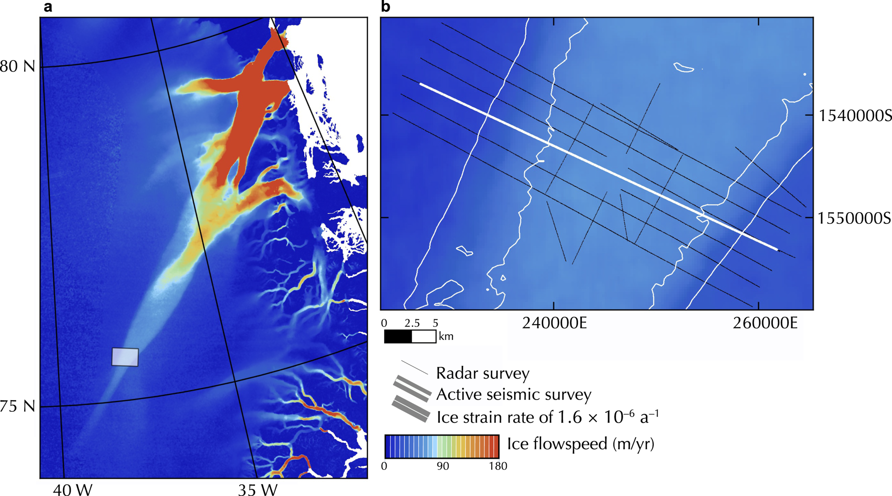
Fig. 1. Ice flowspeed across Greenland from Interferometric Synthetic Aperature Radar (InSAR). (a) NE Greenland Ice Stream study area, indicated with a white box. (b) Geophysical survey at NEGIS. The seismic profile is indicated by the thick white line, and the radar profiles are indicated by the black lines. The ice velocities and strain rates are from 2015 to 2016 Sentinel-1 synthetic aperture radar (Nagler and others, Reference Nagler, Rott, Hetzenecker, Wuite and Potin2015).
It is unlikely that there is temperate ice within the shear margins in our study area. Elsewhere in Greenland and Antarctica, temperate ice can partially determine ice-stream shear-margin location and stability (Suckale and others, Reference Suckale, Platt, Perol and Rice2014; Perol and others, Reference Perol, Rice, Platt and Suckale2015; Meyer and others, Reference Meyer, Yehya, Minchew and Rice2018b). However, the low strain rates (< 5.5 × 10⁻³ a−1) and high degrees of ice incorporation across the shear margins limit temperate ice formation here. This is further supported by GPR surveys across our study area, which do not show any evidence for temperate ice within the shear margins of NEGIS (Christianson and others, Reference Christianson2014; Holschuh and others, Reference Holschuh, Lilien and Christianson2019).
Methods
We use a combination of geophysical techniques to characterize the subglacial environment across the ice stream. Active seismic surveys were used to determine the material properties of the bed. These results were then paired with a GPR survey to determine the bedform length and geometry. We additionally model subglacial water flow under NEGIS to identify possible regions of well-drained bed and quantify the largest-possible channels within our study area. We later use these values to demonstrate that the observed subglacial features cannot be large meltwater channels.
GPR data were collected across both ice-stream shear margins (Fig. 1). GPR data were acquired using a mono-pulse system operating at a center frequency of 2.5 MHz (Welch and Jacobel, Reference Welch and Jacobel2003; Christianson and others, Reference Christianson2014). Details of the GPR processing are presented in Christianson and others (Reference Christianson2014). Corrections to the data include bandpass filtering, time correction for antenna spacing, interpolation to constant trace spacing, two-dimensional time-wave number migration, time correction for spatially variable firn density and a correction for spherical divergence and englacial attenuation.
We conducted a GPS survey of the ice surface in order to determine the bed elevation from the seismic and radar surveys. GPS data were collected using dual-frequency receivers and processed using differential carrier-phase position as implemented in the Track software (Chen, Reference Chen1998). Ice-flow direction and shear strain rates were calculated from InSAR-derived ice surface velocities averaged from 1995 to 2013 (Joughin and others, Reference Joughin, Smith, Howat, Scambos and Moon2010) following eigenvalue-based techniques, detailed in Riverman and others (Reference Riverman2019).
Seismic amplitude analysis
Multichannel seismic reflection data of the basal environment were collected along a 38-km transect across both shear margins of the ice stream. One-kg pentolite explosive charges were detonated ~20 m below the surface at the center of and 480 m off one end of a 48 single-component (vertical) geophone array with a 20-m spacing; the geophone array was then moved forward 480 m, and the shooting sequence was repeated, resulting in twofold seismic data coverage.
We use the measured firn velocity profile of Riverman and others (Reference Riverman2019) to correct for firn structure variations across the ice stream. Firn corrections are particularly important for NEGIS because the firn thickness varies dramatically across the shear margins (Christianson and others, Reference Christianson2014; Riverman and others, Reference Riverman2019). The data were further corrected for surface topography and shot depth. We performed frequency filtering, frequency-wavenumber (FK) filtering and normal moveout correction before stacking the data. Finally, the data were migrated with an ice P-wave velocity of 3700 ms−1. The feature geometries presented below are measured from the migrated seismic sections.
We calculated the bed acoustic impedance (the product of material P-wave velocity and density) across the ice stream based on the amplitude of the seismic reflection from the ice–bed interface to determine the material properties of the ice–bed interface. The processing workflow for the source amplitude corrections started with raw shot data after the bad traces were removed (i.e., no frequency-based filtering was applied to the data in the source amplitude analysis). We restricted the source-receiver offsets used in this analysis to those with angles of incidence less than 10 degrees to minimize the effects of changing bed amplitude with incident angle. We followed the procedures and assumptions of Muto and others (Reference Muto2019) to determine the source amplitude and calculate acoustic impedance at the bed. The source amplitude (A 0) was determined using the direct-path approach of Holland and Anandakrishnan (Reference Holland and Anandakrishnan2009). We chose to use the direct-path approach over the more commonly used multiple-bounce method of Smith and others (Reference Smith2007) because our data lacked strong multiple reflections across most of the ice stream. The path amplitude factor (γ) and primary-ray-path length (d 1) were determined using a one-dimensional velocity model of the glacier that includes both firn and ice (following the procedures of Muto and others, Reference Muto2019).
We calculated the normal-incidence reflection coefficient, R 0, from the amplitudes of the source and the primary reflection (A 0 and A 1, respectively) as:

where γ is the path amplitude factor accounting for geometrical spreading and α is the attenuation constant, chosen here as 2.7 × 10⁻⁴ m−1 (Horgan and others, Reference Horgan, Anandakrishnan, Alley, Burkett and Peters2011). That attenuation constant was calculated for ice across the West Antarctic Ice Sheet, which likely has a similar mean annual air temperature as our site near the summit of Greenland. Horgan and others (Reference Horgan, Anandakrishnan, Alley, Burkett and Peters2011) note that uncertainty in attenuation is the major source of uncertainty in their subsequent seismic amplitude analysis, and this is likely the major source of unquantified uncertainty in our analysis as well.
Of note, there are polarity reversals in A 1 across the ice stream, so R 0 can be positive or negative. We estimate the A 1 and uncertainty for each shot by averaging all available traces within a shot gather and take the standard deviation as the uncertainty.
From R 0 we then calculate the bed acoustic impedance, Z b (Smith and others, Reference Smith2007; Luthra and others, Reference Luthra2017):

where we assume Z ice = 3.33 ± 0.04 × 10⁶ kg m−2 s −1, following Atre and Bentley (Reference Atre and Bentley1993). We estimate the error in Z b for each shot by propagating the uncertainty in A 0, A 1 and α through Eqns. (1) and (2). This does not account for uncertainty in the attenuation constant. We then use the acoustic impedance of the subglacial material to identify its composition based on the known acoustic impedances of commonly observed subglacial materials. Dilated sediments are generally assumed to have an acoustic impedance range of 2.3 × 10⁶–3.85 × 10⁶ kgm−2 s−1 (from Atre and Bentley (Reference Atre and Bentley1993) and also used by Muto and others (Reference Muto2019), Smith (Reference Smith1997) and Brisbourne and others (Reference Brisbourne2017)). Water has an acoustic impedance of 1.49 × 10⁶ kg m−2 s−1.
Following Muto and others (Reference Muto2019) we assume that values of Z b > 3.85 × 10⁶ kg m−2 s−1 correspond to a till porosity of <0.3 and include lodged, non-deforming till. We refer to these regions as ‘consolidated sediments,’ though they may include sedimentary or crystalline bedrock. Values of 2.3 × 10⁶ kg m−2 s−1 < Z b < 3.85 × 10⁶ kg m−2 s−1 correspond to till that is much softer, deformable and saturated with high-pressure water (Atre and Bentley, Reference Atre and Bentley1993; Peters and others, Reference Peters, Anandakrishnan, Alley and Smith2007, Reference Peters2006; Luthra and others, Reference Luthra2017; Muto and others, Reference Muto2019). See Muto and others (Reference Muto2019) for additional details, uncertainty estimates and a more extensive discussion of this technique for calculating acoustic impedance of subglacial materials.
Modeling water flow
Some studies have related bedform development to fluvial sediment transport (Shaw, Reference Shaw2010). Others have linked variations in effective pressure (the difference between ice overburden pressure and water pressure) with sediment transport and bedform development (Iverson and others, Reference Iverson2017). We model water flow under NEGIS using the Glacier Drainage System (GlaDS) model (Werder and others, Reference Werder, Hewitt, Schoof and Flowers2013) to determine if the bedforms observed under NEGIS form via some fluvial process.
Wet bedforms might share some qualitative characteristics with subglacial channels in geophysical surveys, and subglacial channels are thought to form under some shear margins with high lateral strain rates (Perol and others, Reference Perol, Rice, Platt and Suckale2015; Elsworth and Suckale, Reference Elsworth and Suckale2016; Meyer and others, Reference Meyer, Fernandes, Creyts and Rice2016; Platt and others, Reference Platt, Perol, Suckale and Rice2016). We perform hydrologic modeling to constrain the range of channel sizes and locations for this site. By specifying a very high basal melt rate, we put an upper bound on channel size, which can be compared to observed feature morphology to discriminate between wet sediment and water-filled channels.
GlaDS is a 2-D finite-element model that simulates both distributed and efficient drainage networks beneath the ice. R-channels are modeled along the element edges including creep closure, viscous dissipation of heat and supercooling freeze-on, while the distributed system is modeled across the element with a Darcy–Weisbach type flow equation in the form of linked-cavities or sediment depending on the system conductivity. Water is exchanged between the distributed and channelized systems, which allows the subglacial drainage configuration to evolve over time. Details of the model configuration used here, including the model domain and resolution, can be found in Dow and others (Reference Dow, Karlsson and Werder2018). The model domain extends across the entire Greenland Ice Sheet, but is higher-resolution within the NEGIS catchment. Fahnestock and others (Reference Fahnestock2001) found peak melting of >0.1 ma−1 in the anomalous region at the head of NEGIS, whereas melt elsewhere beneath the ice sheet is typically 0–0.01 ma−1. We assign a high value of 0.1 ma−1 to the entire domain. This provides an end-member estimate of water flux within our study area.
Modeling ice infiltration into sediments
We model the depth of frozen sediments accreted to the bottom of the ice column across the ice stream to test the hypothesis that sediment movement under NEGIS is in part controlled by ice infiltration into the underlying sediments. We use the thermomechanical of Rempel (Reference Rempel2008) as implemented by Meyer and others (Reference Meyer, Downey and Rempel2018a) and Meyer and others (Reference Meyer, Robel and Rempel2019) to calculate the steady-state ice-infiltration depth into the till, h. At the base of ice streams underlain by till, ice can infiltrate into the sediments where pore water pressure is low (and therefore effective stress is high) and where the basal melt rate is low. Where effective pressures are above a critical threshold, P f, ice intrudes into the interstitial pore spaces (Rempel, Reference Rempel2008; Meyer and others, Reference Meyer, Downey and Rempel2018a, Reference Meyer, Robel and Rempel2019). The model is derived from first principles and verified experimentally (Rempel and others, Reference Rempel, Wettlaufer and Worster2004; Rempel, Reference Rempel2007, Reference Rempel2008). See Meyer and others (Reference Meyer, Downey and Rempel2018a) for an extended discussion of the derivation and use of this model.
The transient problem can be reduced to an idealized one-dimensional second-order partial differential equation for temperature. Properties of the till layer included here are its porosity ϕ, the variation in ice saturation S i and permeability k with temperature, and the density difference Δρ till between the sediment particles and water ρ. Steady-state infiltration depth satisfies:
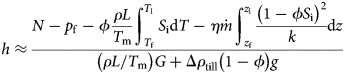
where N is effective pressure, η is water viscosity and $\dot m$ is the melt rate. The terms in the denominator of Eqn. (3) describe the change in vertical pressure exerted across wetting films and buoyancy of the overlying till with infiltration thickness. The temperature gradient through the ice-infiltrated sediments G is approximated as a constant, 0.03 km−1. The numerator includes terms for the effective stress, N at the base of the ice-infiltrated layer. The second term, p f = ρL(1 − T f/T m), is the load supported by the wetting films at the base of the ice-infiltrated layer. The final term in the numerator accounts for deviations of the liquid pressure gradient away from hydrostatic equilibrium. Parameter choices here include ϕ = 0.35, Δρtill = 1650 kg m−3, and T m − T f = 0.031 K, with the ice saturation and permeability modeled using the power laws

with β = 0.53, α = 3.1 and k 0 = 4.1 × 10⁻¹⁷ m2.
The model is quite sensitive to the selected effective pressure, which is difficult to directly measure. GLaDS models effective pressure across our study area, but the resulting modeled effective pressure variations across the ice stream are perhaps unrealistically low in our study area (−0.2 to 0.3 MPa). Instead, we assume that the shear stress, τb, and effective pressure are related at the basal boundary using the Mohr–Coulomb relationship.

where μ is the coefficient of friction, and cohesion is neglected (Iverson and others, Reference Iverson, Hooyer and Baker1998; Minchew and others, Reference Minchew2016; Meyer and others, Reference Meyer, Robel and Rempel2019). The coefficient μ is assumed to be 0.6, following Meyer and others (Reference Meyer, Robel and Rempel2019). We use the basal shear stress approximation from Holschuh and others (Reference Holschuh, Lilien and Christianson2019), which was inverted for using Elmer/Ice (Zwinger and others, Reference Zwinger, Greve, Gagliardini, Shiraiwa and Lyly2007; Gagliardini and others, Reference Gagliardini2013). We assume a geothermal heat flux of 75 mW m−2 from Davies (Reference Davies2013). All of the other model parameter choices follow those of Meyer and others (Reference Meyer, Robel and Rempel2019), as detailed in their Table 1.
Results
Acoustic impedance of the subglacial material across NEGIS generally falls into the range of soft, saturated, dilatant sediments (Fig. 2c). There are several bump-like features along the seismic profile that could be interpreted as subglacial bedforms at km 10, 16, 17, and 33 in Figure 2. Here, we use our co-located radar survey to determine which of these possible bedforms extend up- and down-glacier. One feature in the southern shear margin extends across several radar survey lines (Fig. 3). Another feature in the northern shear margin extends across two radar lines. Other candidate bedforms identified from the seismic survey have less-clear upstream–downstream continuation, so they are not discussed further here. However, we note that higher-resolution radar surveys within this study area are likely to find additional streamlined features. Below we detail properties of these margin bedforms and overlying ice and then compare their locations to modeled meltwater flowpaths and ice infiltration depths.
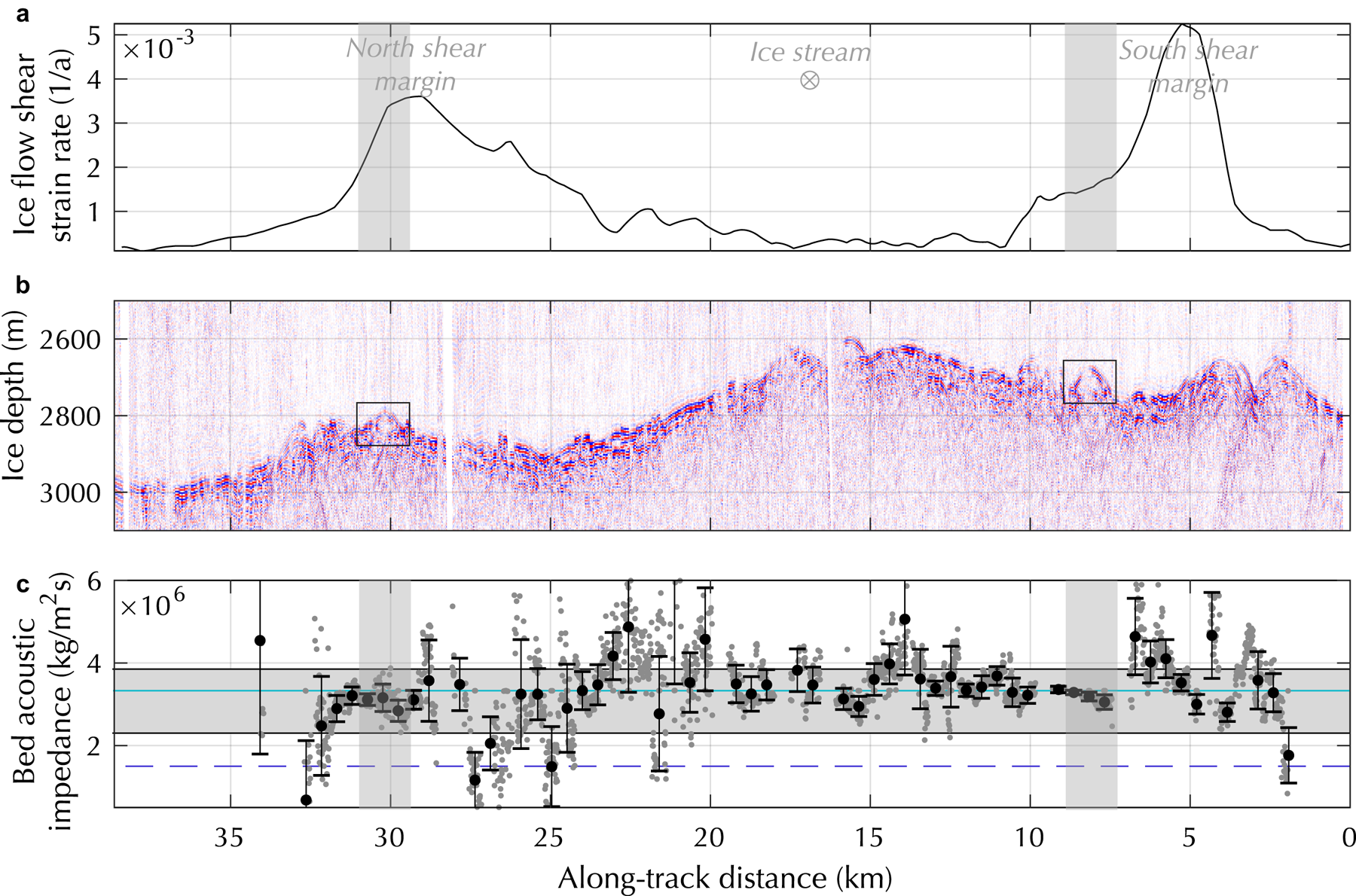
Fig. 2. Subglacial conditions across the NE Greenland Ice Stream from active seismic data. The location in Greenland is shown as the white line in Figure 1b. Gray vertical bands correspond to the subglacial features described in the text. Ice flow within the ice stream is into the page. The features discussed in the text are shown with black boxes. (a) Strain rate across the ice stream resulting from ice flow (Riverman and others, Reference Riverman2019), as measured from Interferometric Synthetic Aperture Radar (Joughin and others, Reference Joughin, Smith, Howat, Scambos and Moon2010). (b) Stacked, unmigrated seismic section showing the basal reflector. The black boxes indicate bedforms described here. Figures 3 and 4 show enlargements of these areas and coincident radargrams. Additional bumps (e.g., at km 17) may be bedforms but are not observed clearly in parallel radar lines upstream or downstream. (c) Acoustic impedance of the subglacial materials, Z B, for each receiver (gray dots) and shot-averaged (black dots). Error bars show one standard deviation of variance for measurements in each shot. Horizontal lines show modeled acoustic impedances for common subglacial materials. The cyan line shows the acoustic impedance of ice. The blue dashed line shows the acoustic impedance of water. Black lines and the filled gray box show values of 2.2 × 10⁶ kg m−2 s−1 < Z b < 3.8 × 10⁶ kg m−2 s−1 correspond to soft, deformable, water-saturated till (Atre and Bentley, Reference Atre and Bentley1993; Smith, Reference Smith1997).
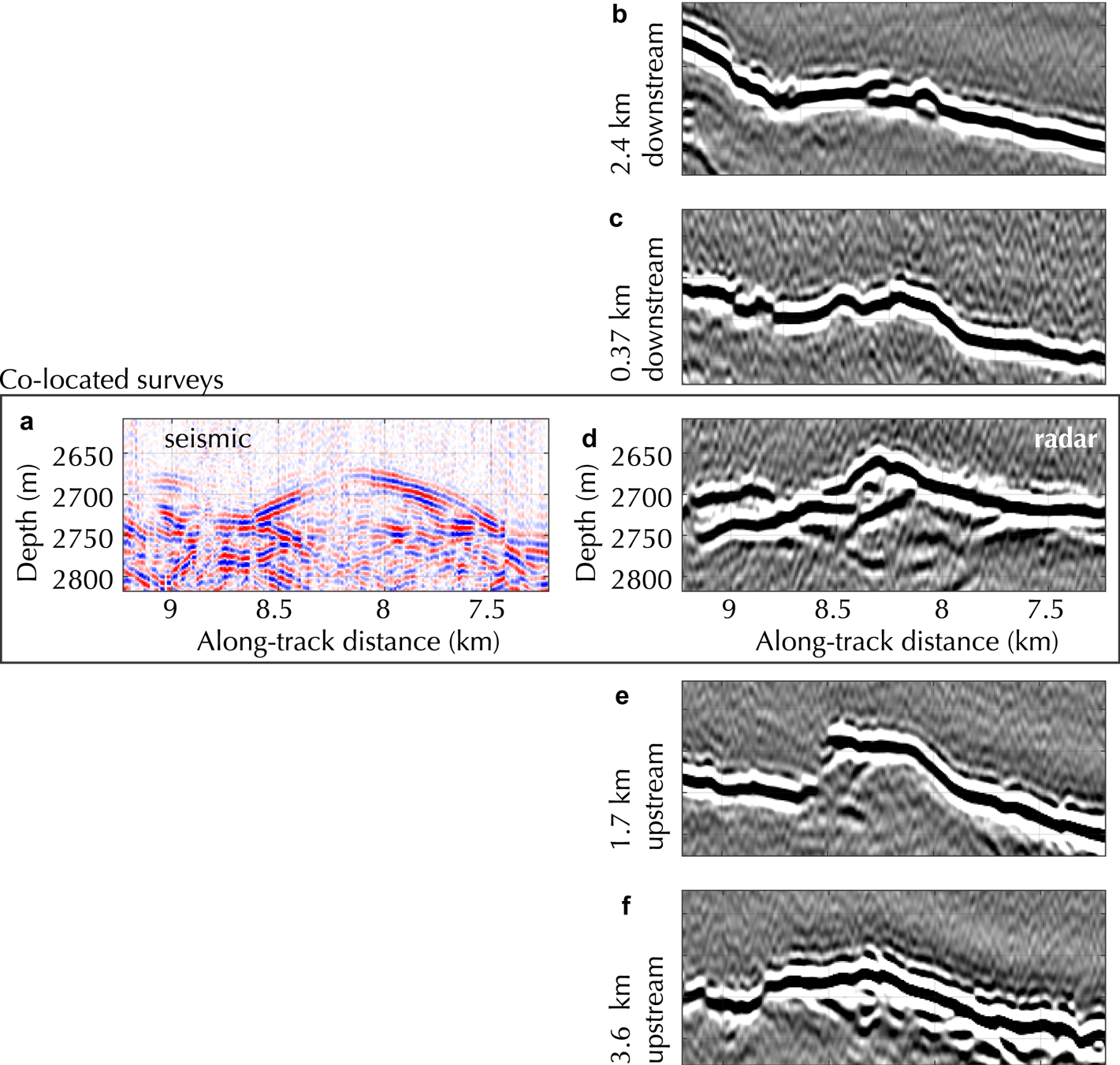
Fig. 3. Seismic and radar lines showing the bed reflector across the southern shear margin of the NE Greenland Ice Stream. Location of the picked bedform is shown in Figure 2. Distances upstream/downstream are relative to the bedform at the seismic line. (a) Active seismic line across the bedform. (b) Radar line 2.4 km downstream from seismic line. (c) Radar line 0.34 km downstream from seismic line. (d) Radar line co-located with seismic line. (e) Radar line 1.7 km upstream of seismic line. (f) Radar line 3.6 km upstream of seismic line. For (b)–(f), the X and Y axes have the same scale as those noted for (d), with slightly shifted positions to center the feature.
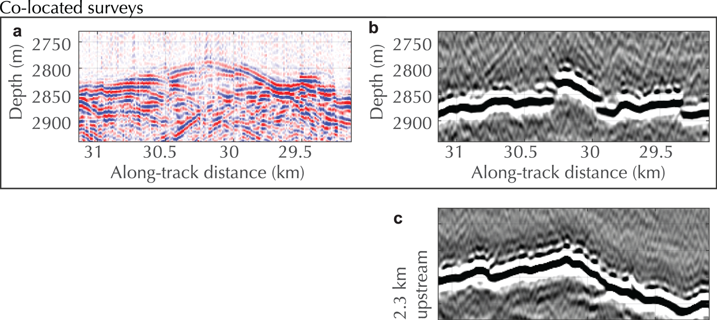
Fig. 4. Seismic and radar lines showing the bed reflector across the northern shear margin of the NE Greenland Ice Stream. Location of the picked bedform is shown in Figure 5. (a) Active seismic line. (b) Radar line co-located with seismic line. (c) Radar line 2.3 km downstream from seismic line. For (c), the X and Y axes have the same scale as those noted for (b), with a slightly shifted position to center the feature.
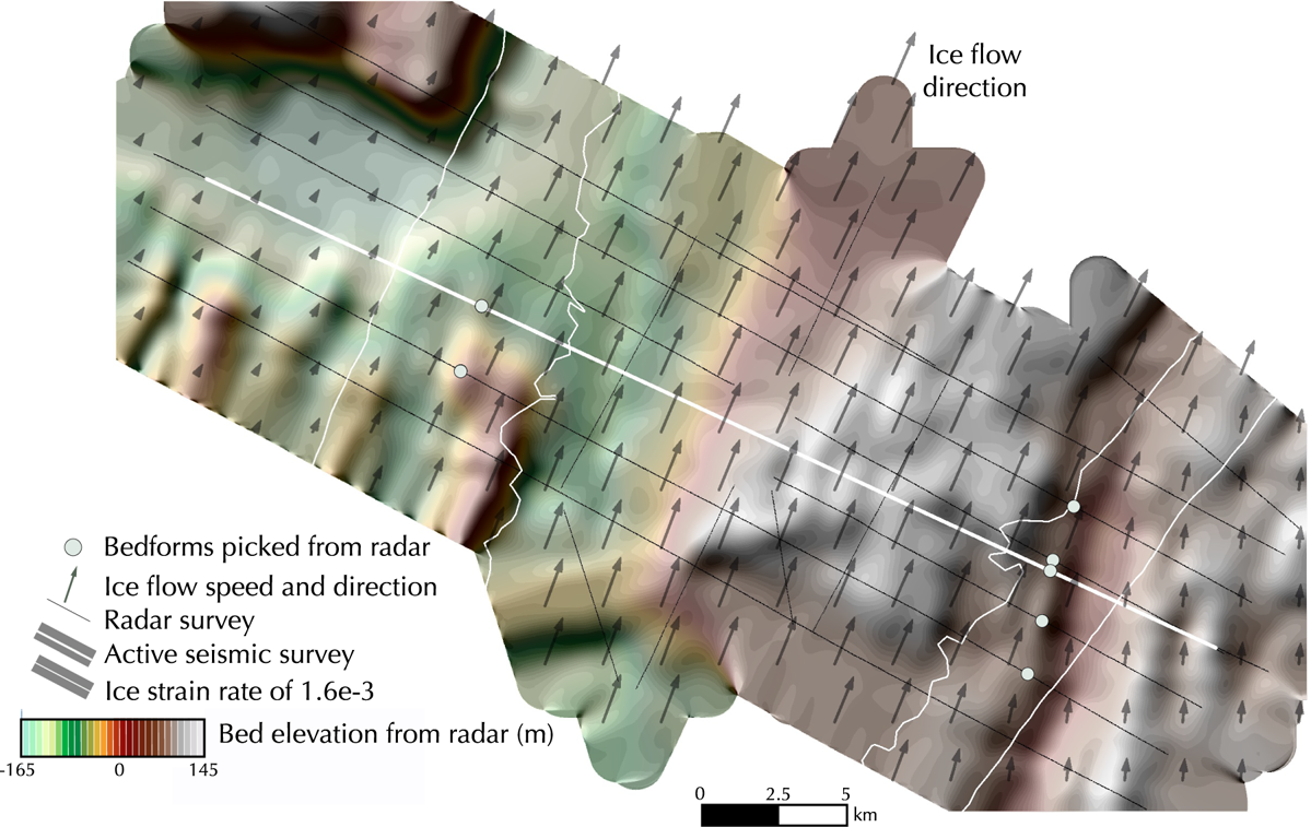
Fig. 5. Map of bed elevation showing picked bedforms (green dots), ice-flow direction (gray arrows, with size indicating flowspeed from 9 to 51 ma−1), seismic survey (white thick line), and radar survey (gray thin line). Areas bounded by the thin white line show where the ice-flow strain rate is greater than 1.6e−3 a−1. Site location corresponds to the inset in Figure 1a and covers the same region as Figure 1b.
Margin bedforms
The two major subglacial features we identify in the seismic stacked section are labeled with black boxes in Figure 2b. The subglacial bedforms are 40–60 m high (assuming an ice P-wave velocity of 3700 ms−1) and are 400–700 m wide. Near-offset seismic acoustic impedance data (Fig. 2c) show that each marginal bedform is composed of soft, water-saturated till.
Coincident radargrams from Christianson and others (Reference Christianson2014) show undulations in the bed that correspond with the seismically identified soft, deformable bedforms (Fig. 2). Radar profiles upstream and downstream of the seismic survey provide constraints on the length of features, although the length estimates are limited by the along-flow spacing of our radar lines (Figs 3 and 4).
The feature in the southern shear margin is one ice thickness instream of the location of maximum strain rate. It is 670 m wide and 62 m tall (inferred from the migrated seismic and radar surveys). It is likely visible across five of our radar transects, indicating that it is ~6.6 km long. We do not seismically detect any large internal reflectors within the bedform. This suggests that the bedform is composed of homogeneous till with no major variations in density or seismic velocity. The acoustic impedance of at least the upper few meters of the feature is quite low: ~3.1 × 10⁶ kg m−2 s−1, indicating high-porosity, water-saturated till. On the south side of the feature, the bed transitions to stronger material with a higher acoustic impedance (~4.6 × 10⁶ kg m−2 s−1) within 500 m of the bedform. We find no such boundary on the northwest side of the bedform (toward the center of the ice stream). Figure 5 shows the location of the bedform relative to ice-flow direction and shear margin position. The bedform is roughly flow-parallel, and ice-flow velocity increases significantly along the length of the feature as the ice enters the ice stream: from 29.5 ma−1 at the most upglacier radar line to 51.9 ma−1 at the most downglacier radar line.
The feature in the northern shear margin is 1 km outboard of the point of maximum strain rate. The acoustic impedance of the feature is ~3.1 × 10⁶ kg m−2 s−1, indicating high-porosity, water-saturated till. This is the same acoustic impedance as the bedform in the southern shear margin. Where crossed by the seismic survey, the bedform is 410 m wide and 44 m tall. It is visible in two of our radar transects, indicating that it is at most 5.1 km long. There are no prominent internal reflectors within this bedform, suggesting that it is composed of homogeneous till with no major increases in acoustic impedance at the resolution of our seismic survey. The feature is in a broad region of low acoustic impedance, where soft deforming sediments are pervasive. Ice flowspeed does not change significantly along the length of the feature, with flowspeeds of ~39 ma−1. This feature is roughly flow-parallel (see Fig. 5).
Radar brightness across the subglacial features (presented in Christianson and others, Reference Christianson2014, but not detailed further here) is varied, with no clear pattern. However, we would not expect to see a strong correlation between seismic and radar reflection strength across features because of differences in the resolution of the systems as well as differences in the physical features of the subglacial environment that result in reflections. We also note that these features are very close to the horizontal resolution of the radar system: the Fresnel zone of the 2.5 MHz radar system is 416 m (using an electromagnetic wave velocity of 170 m($\rm u$ s)−1) and 312 m for the seismic system (using a P-wave velocity of 3700 ms−1 and a seismic frequency of 100 Hz). Additionally, the seismic data have a higher vertical resolution, with a theoretical (1/4 wavelength) resolution of 9.25 m, compared to the 17 m vertical resolution of the radar system. As such, we do not expect the radar reflection brightness to mimic the patterns of acoustic impedances reported here.
Meltwater routing and sediment-entrained ice depth
The GLaDS subglacial hydrology model results show that even under end-member high melt rates, much of the water movement through this region is within the distributed system. Only limited regions of continuous channelization are observed in model results. The greatest degree of channelization occurs in the shear margins of the ice stream (Fig. 6b), consistent with previous water-routing studies (Karlsson and Dahl-Jensen, Reference Karlsson and Dahl-Jensen2015). The water flow modeling work shown here provides no evidence for the role of water movement in bedform development. The location of strongest discharge and channelization does not correlate with bedform location (Fig. 6b). However, the bedforms described here have too large of a cross-sectional area (>7000 m2) to be Rothlisberger channels.
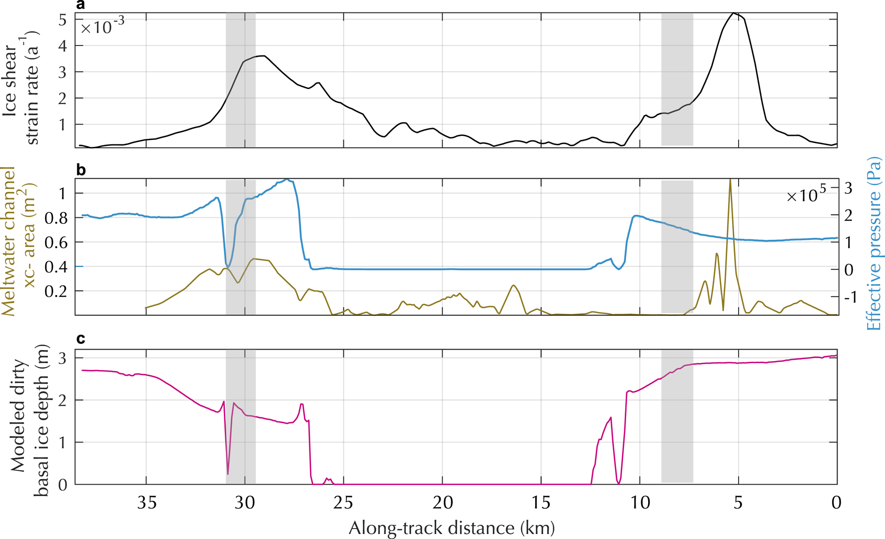
Fig. 6. Modeled meltwater flow across NEGIS. Gray bands indicate the location of bedforms presented here. (a) Location of the NEGIS shear margins, from the ice-flow strain rate. (b) The left axis and yellow line show meltwater channel cross-sectional area from GLaDS modeling. The right axis shows effective pressure at the same locations, as calculated from an ice-flow modeling inversion for basal shear stress. (c) Modeled ice infiltration depth into sediments (forming dirty basal ice layers) using the effective pressures presented in pannel b.
We have also modeled the steady-state ice-infiltration depths across the ice stream. Model results show that debris-rich ice depth decreases as ice crosses the shear margin and flows into the ice stream (Fig.6c). As modeled effective pressures decrease along flowlines moving into the ice stream, basal ice layers may melt and deposit sediments. In the southern shear margin, the location of the bedform (km 8 in Fig. 6) corresponds with the location where modeled steady-state ice infiltration depths first decrease, suggesting that sediment is ‘dropped’ or melted out of the ice column. In the north shear margin, the bedform is also in a broad region where modeled sediments are being deposited from the overlying ice column.
Discussion
Our results show two possible bedforms beneath the NEGIS shear margins. These bedforms are composed of soft, deformable, water-saturated sediments. Other features are visible in the seismic section that may be bedforms, but in the absence of higher-resolution radar data, we are reticent to speculate on their properties.
The size and location of Feature 1 in the southern shear margin are similar to those of features that Stokes and Clark (Reference Stokes and Clark2002) classified as ice stream margin moraines, and correspond most closely to the lateral shear moraines of Batchelor and Dowdeswell (Reference Batchelor and Dowdeswell2016). We thus conclude that this is a lateral shear moraine. To the best of our knowledge, this is the first subglacial observation of such a feature. This feature can provide insights into the ice-flow processes necessary to form the lateral shear moraines of previously glaciated landscapes.
Possible formation mechanism
There is little consensus on a universal formation model for marginal moraines, though many have been proposed (as summarized in Stokes and Clark, Reference Stokes and Clark2002; Hindmarsh and Stokes, Reference Hindmarsh and Stokes2008). These features may form through a similar mechanism to drumlins and mega-scale glacial lineations within the ice stream; however, this does not explain their preferential formation within the shear margins nor their size differences from features found within regions of fast flowing ice (marginal features are generally wider and longer (Batchelor and Dowdeswell, Reference Batchelor and Dowdeswell2016)). For this reason, we focus here on formation mechanisms unique to the shear margins. Below we briefly summarize several previously proposed marginal moraine formation mechanisms and address their relevance to our observations. We then put forward our preferred theory by which sediment that is well-coupled with and entrained in basal ice melts out within the shear margins.
Shear marginal moraines may form at the boundary between warm-based and cold-based ice, arising from thermally controlled differences in erosion rate (Dyke and Morris, Reference Dyke and Morris1988; Kleman and Borgstrom, Reference Kleman and Borgstrom1994). This model is unlikely to be relevant for NEGIS. Our data, as well as those synthesized by MacGregor and others (Reference MacGregor2016), show a thawed bed under the ice stream and outside the shear margin to the south, so a thermal boundary cannot be important for the southern shear margin bedform. Regional analysis shows the possibility of a frozen bed outside of the northern margin (MacGregor and others, Reference MacGregor2016), but Christianson and others (Reference Christianson2014), Holschuh and others (Reference Holschuh, Lilien and Christianson2019), and this study have found evidence for subglacial water in the region. Thus, we conclude that these marginal bedforms did not form because of the effect of thermal boundaries on subglacial erosion rates. We also note that it is unlikely that the thermal regime of this area has recently shifted (Keisling and others, Reference Keisling2014).
Elsewhere, shear margin moraines have been found co-located with a topographic step (with the core of ice stream flow sitting 40 m below the surrounding topography) (Stokes and Clark, Reference Stokes and Clark2002) suggesting that till is excavated from within the ice stream and deposited in the margins. We find no such topographic step across the ice stream (Fig.5), so the source of the till within the marginal bedforms could be external to the ice stream, and there is no clear evidence to support the model that till is excavated from the ice stream interior and deposited within the shear margins.
Shear marginal moraines may also form in regions of ice flow compression or ablation. Hindmarsh and Stokes (Reference Hindmarsh and Stokes2008) present a quantitative model where the ice stream lateral moraines are formed via differential erosion rates related to lateral variations in the ice stream velocity. In their model, subglacial till deposition occurs where there is surface ablation or compressing flow. At NEGIS, we are well within the accumulation zone so would not expect till deposition due to surface ablation. Additionally, the bedforms observed here are within regions of extensional flow (as shown in Fig. 7b of Riverman and others (Reference Riverman2019)). As a result, from the Hindmarsh and Stokes model (Reference Hindmarsh and Stokes2008) we would expect slight erosion of till within the shear margins of NEGIS.
Alternatively, we hypothesize that ice–till coupling across the shear margins and ice infiltration into the sediments collectively contribute to the deposition of sediments within the shear margins of NEGIS. Strong coupling between ice and sediment favors till deformation, whereas decoupling across ice-contact water favors rapid basal motion but reduced till deformation (e.g., Iverson and others, Reference Iverson, Hanson, Hooke and Jansson1995; Fischer and Clarke, Reference Fischer and Clarke2001). The strong velocity variations seen across this area suggest that there are changes in subglacial effective pressure, with areas of low effective pressure lubricating fast ice flow. As ice flows across the shear margins on NEGIS, effective pressure drops and the degree of ice–till coupling likely decreases, resulting in till deposition in the shear margins. Similarly, ice infiltration into sediments varies with changing effective pressures. Figure 6b shows our estimates for effective pressure across the ice stream assuming the Mohr–Coulomb relationship. Ice can infiltrate into sediments where the effective pressures are high (Rempel, Reference Rempel2008; Meyer and others, Reference Meyer, Downey and Rempel2018a). These sediments can later be deposited as the effective pressures decrease and more rapid basal sliding initiates. Our ice-infiltration depth modeling efforts show that the location of observed subglacial bedforms corresponds to locations where we would expect to see sediments accumulating due to decreases in ice-infiltration depth.
A similar theoretical model has been previously applied to the formation of drumlins at Múlajökull, Iceland (Iverson and others, Reference Iverson2017). Sediments there are thought to be entrained in the basal ice at the head and flanks of drumlins during quiescent flow due to high effective pressures. During surge events, subglacial effective pressures drop, sediments are deposited and the drumlins migrate downglacier. Here, we propose a similar model of sediment movement via variations in effective pressure. However, instead of temporal variations in effective pressure driving sediment movement, we propose that spatial variations in effective pressure are responsible for the differential till erosion and deposition rates.
Our hypothesis for bedform formation within the shear margins could explain why shear marginal bedforms are relatively rare across the paleo-record: we would expect to see them form only where there is strong ice-flow advection across ice stream shear margins (i.e., at locations where the ice stream is widening) and where there are strong variations in effective pressure across the shear margin.
It is difficult to fully propose a theory for the formation of these ice stream margin features without higher-resolution geophysical data to constrain their geometries. We find it likely that effective pressure variations, which drive differential entrainment and transport rates, are at play, but we currently have little means to test this hypothesis further.
Conclusions
Our geophysical surveys across the North East Greenland Ice Stream (NEGIS) reveal what we believe to be the first shear margin moraine observed under a margin of an active ice stream. This offers a valuable laboratory for future study of the formation and evolution of these enigmatic features of the paleo-record.
The observed bedforms are composed of saturated, soft, high-porosity till with a low acoustic impedance, and the orientation of the features is flow-parallel. We hypothesize that bedforms are the result of preferential deposition of till within the shear margins resulting from variable till coupling and ice infiltration into sediments. Future modeling and observational work are necessary to more completely describe the formation of the basal features across the shear margins of NEGIS.
Acknowledgments
K.R. was supported by the National Science Foundation Graduate Research Fellowship under Grant No. DGE1255832, with additional funding from the University of Oregon Department of Earth Sciences. K.C. was supported by NASA grant NNX16AM01G. C.D. was supported through Natural Sciences and Engineering Research Council of Canada (RGPIN-03761-2017) and Canada Research Chairs Program (950-231237). B.R.P. was supported by NASA grant NNX15AH84G and NSF grants PLR-1443190 and AGS-1338832; R.B.A. acknowledges support from PLR-1738934. All authors except C.D. received support from NSF grant OPP-0424589. Logistical support was provided by CH2MHILL Polar Services, the New York Air National Guard, Kenn Borek Air, the Alfred Wegener Institute for Polar and Marine Research, and the North Greenland Eemian Ice Drilling Project. Thank you to C. Meyer and A. Rempel for many useful conversations and comments on the manuscript. All data presented here are available upon request of the corresponding author.


 Open access