Introduction
Remote sensing of glaciers and ice sheets for mass-balance studies has progressed considerably over the last few decades due to the many new instruments and techniques available (Reference Wingham, Ridout, Scharroo, Arthern and ShumWingham and others, 1998; Reference McConnellMcConnell and others, 2000). However, aerial photography is still useful for smaller glaciers with data sometimes going back 450 years. Mass-balance measurements based on remote sensing are called the geodetic (or cartographic) method, where the cumulative net balance is calculated from glacier surface elevations measured in different years. This method is far less expensive and time-consuming than the traditional method based on field measurements, especially since the introduction of digital photogrammetry and digital terrain models (DTMs).
The traditional method of mass-balance measurements is based on annual field measurements and is determined by interpolating results from a number of in situ point observations. Thismethod is both time-consuming and expensive, and globally long-term mass-balance records are sparse.
The Norwegian Water Resources and Energy Administration (NVE) has photographed glacier areas in Norway over several decades. A recent study of more than 120 glacier units in Norway has revealed large local and regional changes in glacier behaviour during this period (Reference SortebergSorteberg, 1998; Reference Andreassen, Kjøllmoen, Knudsen, Whalley and FjellangerAndreassen and others, 2000). Whereas most of the glaciers were retreating or were stable, quite a few were advancing. To obtain further detailed information about the glacier changes, the geodetic method has been applied to many glaciers in Norway (cf. Reference HaakensenHaakensen, 1986; Reference ØstremØstrem and Tvede, 1986; Reference Kjøllmoen and ØstremKjøllmoen and Østrem, 1997; Reference AndreassenAndreassen, 1999; Reference Østrem and HaakensenØstrem and Haakensen, 1999). In Norway we have also measured mass balance on 40 glaciers totalling 473 years of measurements (including 1999/2000). Since many of these glaciers have been mapped twice or more, we have a unique opportunity to compare the geodetic and traditional methods.
In this paper we discuss the geodetic method and apply it to seven glaciers in Norway. The results are compared with observed and estimated mass-balance records. Short-term records are extended by regression analysis of traditional measurements carried out at other glaciers. The accuracy of the methods is discussed. Our objectives are to present net balance values for both methods and the discrepancies between them, and to compare the geodetic and traditional methods.
Setting
The investigated glaciers are all located in Norway: four in the south and three in the north. Figure 1 shows the location of the glaciers. Tables1 and 2 list the available data and some of the geographical parameters. The selected glaciers have been mapped in detail from aerial photographs at least twice since the 1960s, and traditional mass-balance measurements have been conducted for some or all of the periods between mappings.
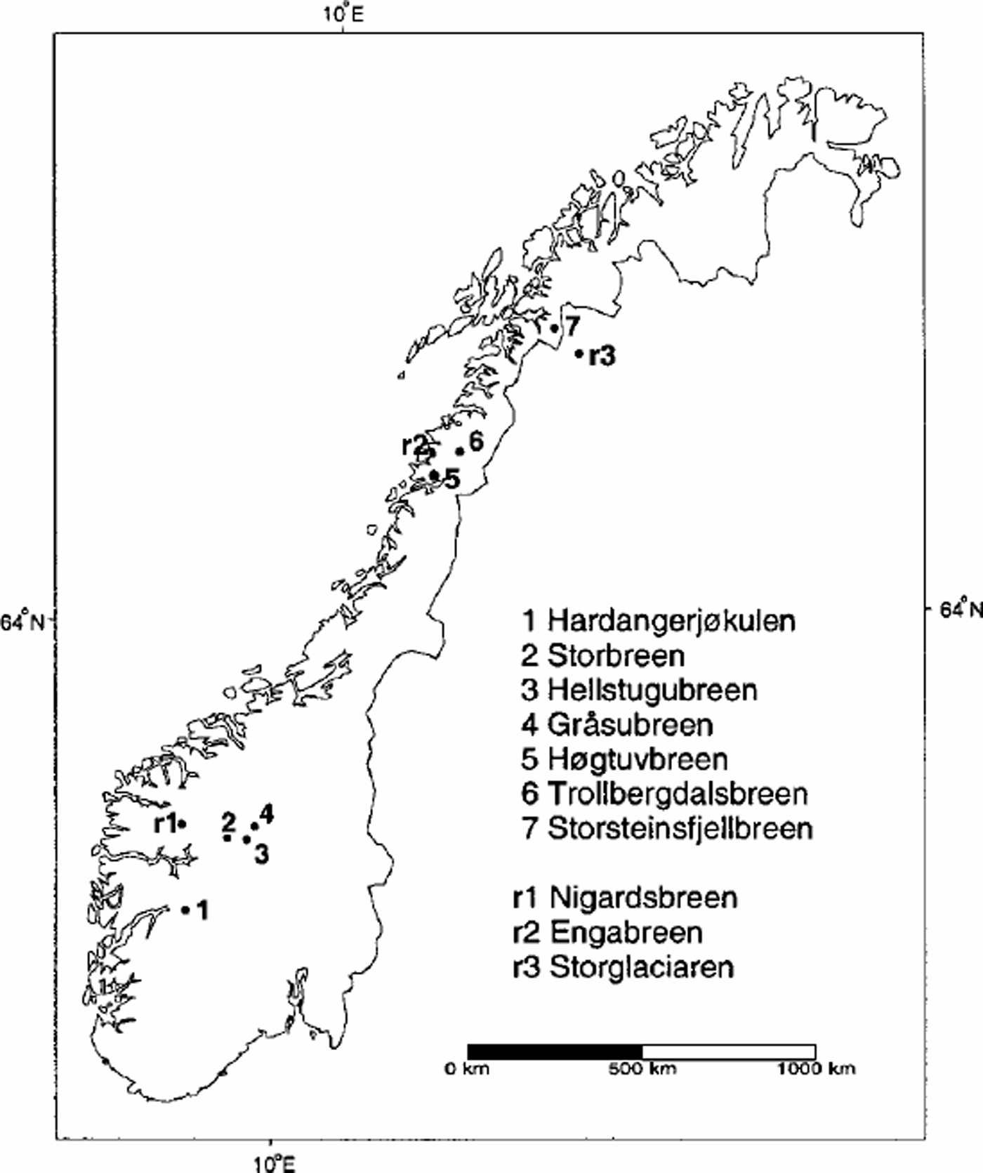
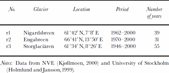
Fig. 1. Location map showing study glaciers (1–7) and reference glaciers (r1–r3).
Table 1. Available data material for the studied glaciers
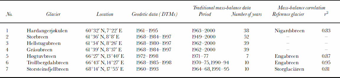
Table 2. Details of aerial photographs and maps/DTMs and glacier characteristics
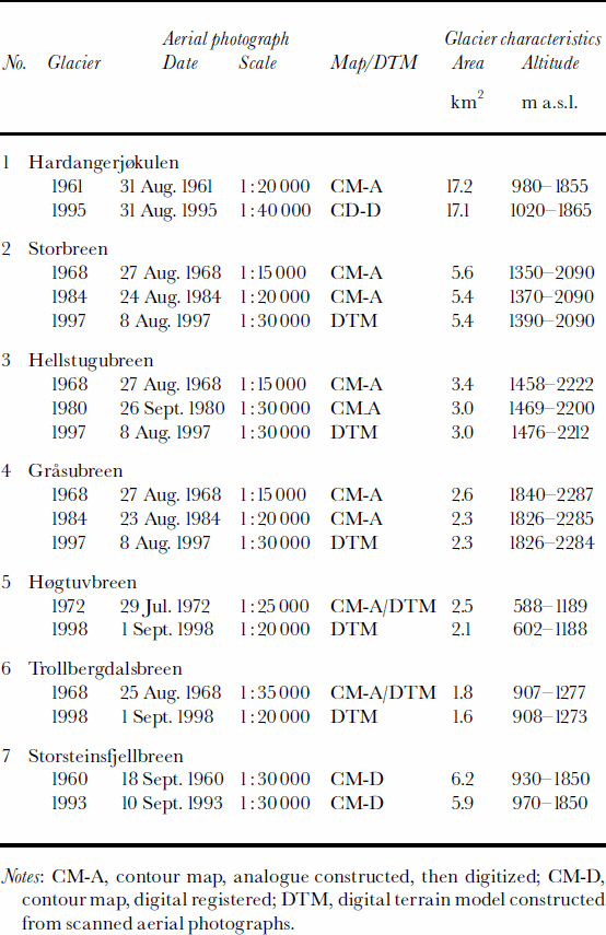
Mass-balance measurements of the study glaciers in southern Norway have shown a systematic decrease in both winter and summer balance that is evident from Hardanger-jÖkulen in the west to Gråsubreen in the east due to an increasingly continental climate (cf. Reference KjøllmoenKjøllmoen, 2000). The winter and summer balances at Gråsubreen are only one-third and one-half of the respective winter and summer balances measured at Hardangerjøkulen. Rembesdalsskåka (17 km2) is a western outlet glacier from the Hardangerjøkulen ice cap (73km2) located in western Norway (Fig. 1). We refer to this glacier outlet as Hardangerjøkulen in this paper, since this is the name previously used when reporting the traditional mass-balance results. The outlet has a long-term mass-balance record and has been mapped in detail twice. Storbreen, Hellstugubreen and Gråsubreen are all small glaciers situated in Jotunheimen, a mountain area in central southern Norway. The glaciers have long-term mass-balance records and have been mapped in detail three times since 1968. Storbreen (5.4 km2) is an east- facing valley glacier and Hellstugubreen (3.0 km2) is a north-facing valley glacier. Gråsubreen (2.2 km2) is northeast-facing, has a polythermal temperature regime and is the most continental glacier in this study.
The three study glaciers in northern Norway all have short-term records of traditional mass balance (7–10 years). They form a south–north transect in northern Norway. According to the direct measurements, both the winter balance and summer balance decrease with increasing latitude. The annual mass exchange at Storsteinsfjellbreen was less than one-half that at Høgtuvbreen. The small eastfacing valley glacier Høgtuvbreen (2.0 km2) is part of a larger glacier complex located 25 km south of Engabreen in northern Norway. Trollbergdalsbreen (1.6 km2) is a small east-facing valley glacier located 30 km northeast of Engabreen. The northernmost glacier in this study, Storsteinsfjellbreen (5.9 km2), is a southeast-facing valley glacier located northeast of Narvik in northern Norway.
Data And Methods
Aerial photographs and DTMs
All the DTMs were constructed using stereophotogrammetry from vertical aerial photographs, but the methods have changed over the years. The maps made in the 1960s and 1970s, and some of those in the 1980s, were constructed using analogue photogrammetry. The resulting maps were made at a scale of 1:10 000 or 1:20 000 (depending on the size of the glacier), with 10m contour intervals (Òstrem, 1986). In the 1980s and 1990s, analogue stereo plotters were used, but the elevations were generally registered with a digital encoder. From the end of the 1990s the DTMs were usually constructed directly from scanned aerial photographs. Professional constructors at Fjellanger WiderÖe carried out the digital photogrammetry work.
Existing analogue contour maps were digitized and converted to regular grids. A triangular irregular network (TIN) was constructed from the digitized contour data and interpolated to a regular grid. In other cases, kriging interpolation was used to produce grids. Interpolation methods and cell sizes were tested and compared to see how this influenced the resulting grids. Generally, the results depended neither on the interpolation technique nor on the chosen cell size, except for the smallest glaciers, such as Trollbergdalsbreen. In areas with low slopes, such as ridges and depressions on plateau glaciers, interpolation from digitized contour lines can produce flat areas. At Hardangerjøkulen, break-lines defining breaks in the slopes were used to produce a realistic grid.
The original 1968 map of Trollbergdalsbreen and the 1972 map of Høgtuvbreen had a low accuracy due to poor ground control. Therefore, when DTMs were constructed from the 1998 vertical photographs of these glaciers, new digital terrain models were constructed from the 1968 and 1972 vertical photographs as well. The pair of DTMs for each glacier was developed using the same control points.
Geodetic mass-balance calculations
The surface elevation change was calculated by subtracting the DTMs on a cell-by-cell basis. The calculated altitude difference represents a volume in glacier ice, firn and partly snow. The density and the thickness of the firn and snow layers in the accumulation areas were unknown, and no field data were available. When a glacier is in steady state, the density profile from the surface to the firn/ice transition remains unchanged (Reference BaderBader, 1954), and we assume that the density profiles are unchanged during the mapping interval. The change in water equivalents was found by multiplying the difference grid with the density of ice, 900 kgm–3 (Reference PatersonPaterson, 1994). Finally, the volume-change results were modified to account for any difference in additional melting that could have occurred between the date of photography and the end of the melting season. This was necessary for comparing the results with traditional cumulative mass-balance data. However, in most cases the photography was done close to the end of the ablation period, and any difference in melt was neglected.
Traditional mass-balance measurements
Annual mass balance has been monitored at various periods for all the studied glaciers (see Table 1). While new geodetic methods have developed rapidly, the traditional methods are nearly unchanged throughout the observation period on the studied glaciers. The mass balance was calculated between two successive summer surfaces, the so-called stratigraphic method. Based on many years’ experience of measurements, the observation network has been reduced without affecting the accuracy of the resulting balance calculations and the final result. A detailed description of the traditional measurements and methodology is found in Reference Østrem and BrugmanØstrem and Brugman (1991) and Reference KjøllmoenKjøllmoen (2001).
Extrapolating traditional mass-balance data series
To compare volume changes calculated from DTMs with volume changes calculated from traditional mass-balance records at the three glaciers in northern Norway, the annual records had to be extended. The first year of the comparison period at Hardangerjøkulen lacked observations and was estimated. The mass-balance records of Storbreen, Hellstugubreen and Gråsubreen covered the whole period between the DTMs. Annual mass-balance data were estimated for the years when linear regression analysis was not used. The long, continuous mass-balance records of Engabreen (1970–), Nigardsbreen (1962–) and Storglaciären (1946–) were used as reference series (Fig. 1; Table 3). Good correlation with the reference series was found for all the glaciers. The coefficient of determination, r2, varied from 0.81 to 0.95 (Table1).
Table 3. Traditional mass-balance data for the reference glaciers used for correlation
Uncertainties
The accuracy of the final geodetic result is affected by a number of factors. One of these is the photo scale of the verticals, a larger scale (lower flying height) giving a smaller standard error. Other factors are the accuracy of the geodetic reference network, the photogrammetric construction, the quality of the aerial photographs and, in particular, the characteristics of the snow surface. Constructing contour lines over snowy areas is always difficult due to the poor contrast, which gives inaccurate results. Digitizing analogue maps introduces horizontal random errors relating to the accuracy of the digitizer and the condition of the analogue manuscript. Coordinate system transformations, interpolation of DTMs and grid overlay operations introduce errors (Reference BurroughBurrough, 1986). Creating grids from digitized contour lines may produce step-like features due to the large number of closely spaced data points at the same altitude. Furthermore, we have to take into account the glaciologic errors. Changes in the density profiles will cause errors in our calculations. Estimating the additional melt can be difficult if we have no stake measurements and little information about glacier melting, especially when the glacier has a highmass turnover.
The propagation of errors in the geodetic method throughout the data handling and analysis, G, can be expressed as:
where g1 – gn are the individual errors. The main errors are g1, the error in elevation grid1; g2, the error in elevation grid2; and g3, the error resulting from assuming an unchanged density profile and estimating the additional melt. We have estimated g1 – g3 for each DTM comparison. The estimated standard error in elevation in the DTMs, g1 and g2, was ±0.5–2.0m. DTMs constructed by digital photogrammetry with proper ground control will have an accuracy of ±0.5–1.0m. Old contour maps or DTMs with poor ground control will have higher errors, >±1.0m. The 1961 DTM of Hardangerjøkulen was estimated to have an accuracy of ±2.5m. The error of the additional melt and the density profile, g3, varied between ±0.3 and ±1.0m. The size of g3 was mainly dependent upon how well we could estimate the additional melt. The potential density error was difficult to estimate. In total, we calculated standard errors of the geodetic method, G, varying from ±1.4 to ±3.0m, or ±1.3 to ±2.7mw.e. The highest standard errors were obtained where the maps/DTMs were constructed from different control points and/or were considered to have a low accuracy because of poor contrast in the snowy areas. Ideally, if we have a pair of very high-quality DTMs of a glacier that is close to steady state between mappings, and we know the additional melt, we can obtain a standard error for the geodetic method of about ±0.7mw.e.
The uncertainties in the traditional mass-balance measurements are dependent on both the accuracy of the point observations and the conversion of point values to spatially distributed values. When the uncertainty in point measurements is thought of as random, the uncertainty in converting point values to spatial averages may introduce systematic errors. It is difficult to quantify the accuracy of the individual factors. The average accuracy of the annual net balance was subjectively estimated as ±0.2–0.4mw.e. The accuracy of the estimated net balance was obviously higher and was estimated as ±0.6mw.e. for Høgtuvbreen and Trollbergdalsbreen, and ±0.65mw.e. for Storsteinsfjellbreen due to a lower correlation with the reference series. Assuming that the error for each year is truly random, the standard error for the cumulative period, T, can be calculated as:
where x is the number of years with measured values, t1 is the average standard error for each year with measured mass balance, y is the number of years with estimated net balance and t2 is the average standard error for each year with estimated balance. When we estimated an average annual value, we assumed that some years have lower accuracy and some have higher accuracy. We usually assumed that the accuracy had been the same over the entire period, since the methods are almost unchanged over this period. Certainly, this could have been done in a more detailed and sophisticated way for each observation year, but the estimates obtained would be somewhat subjective. The calculations gave total standard errors of ±1.3mw.e. for the 29 year periods of Storbreen, Hellstugubreen and Gråsubreen, and ±3.5 mw.e. for the 33 years of estimated and measured mass balance at Storsteinsfjellbreen.
Comparison Of Results From The Geodetic And Traditional Methods
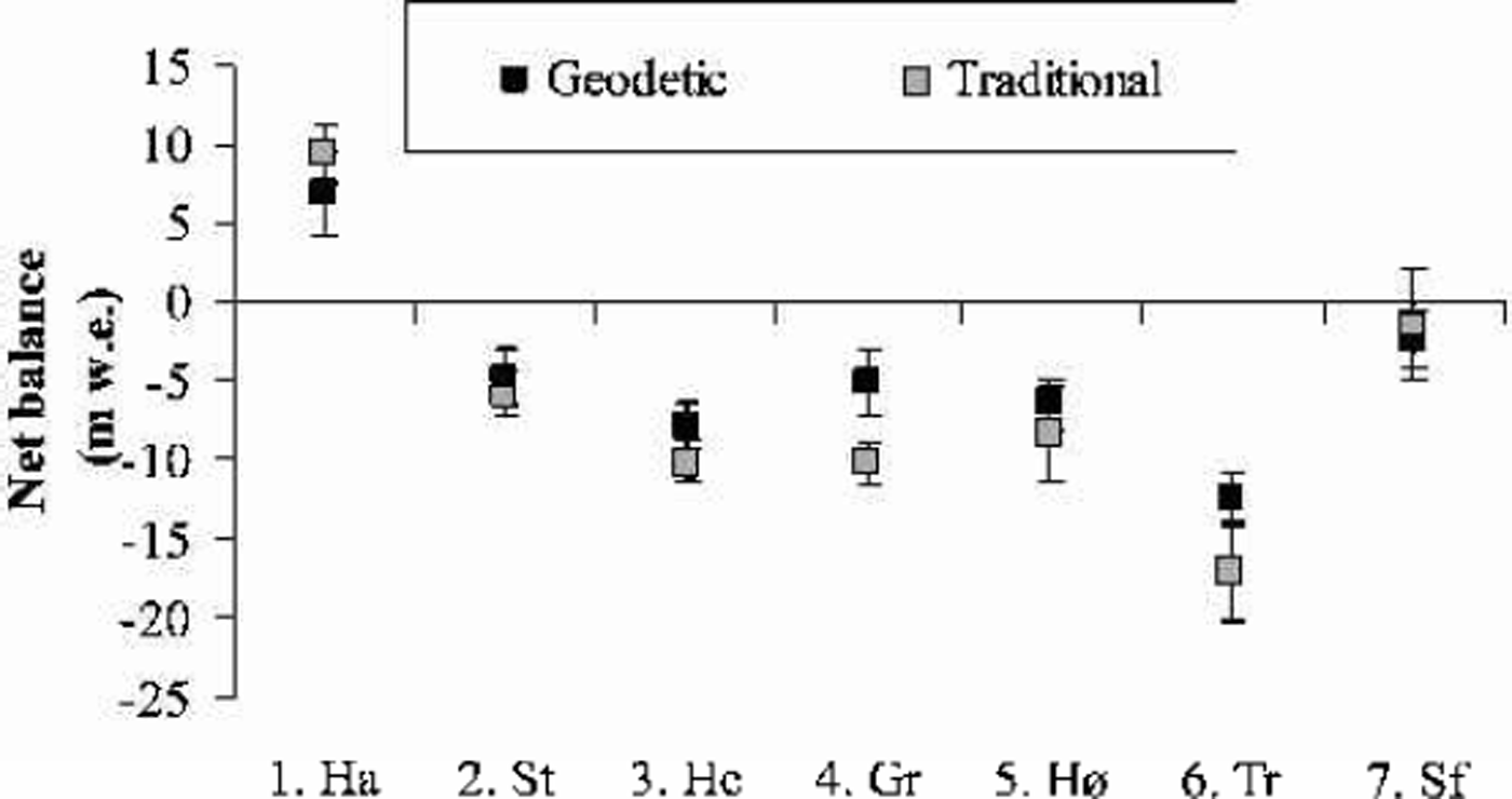
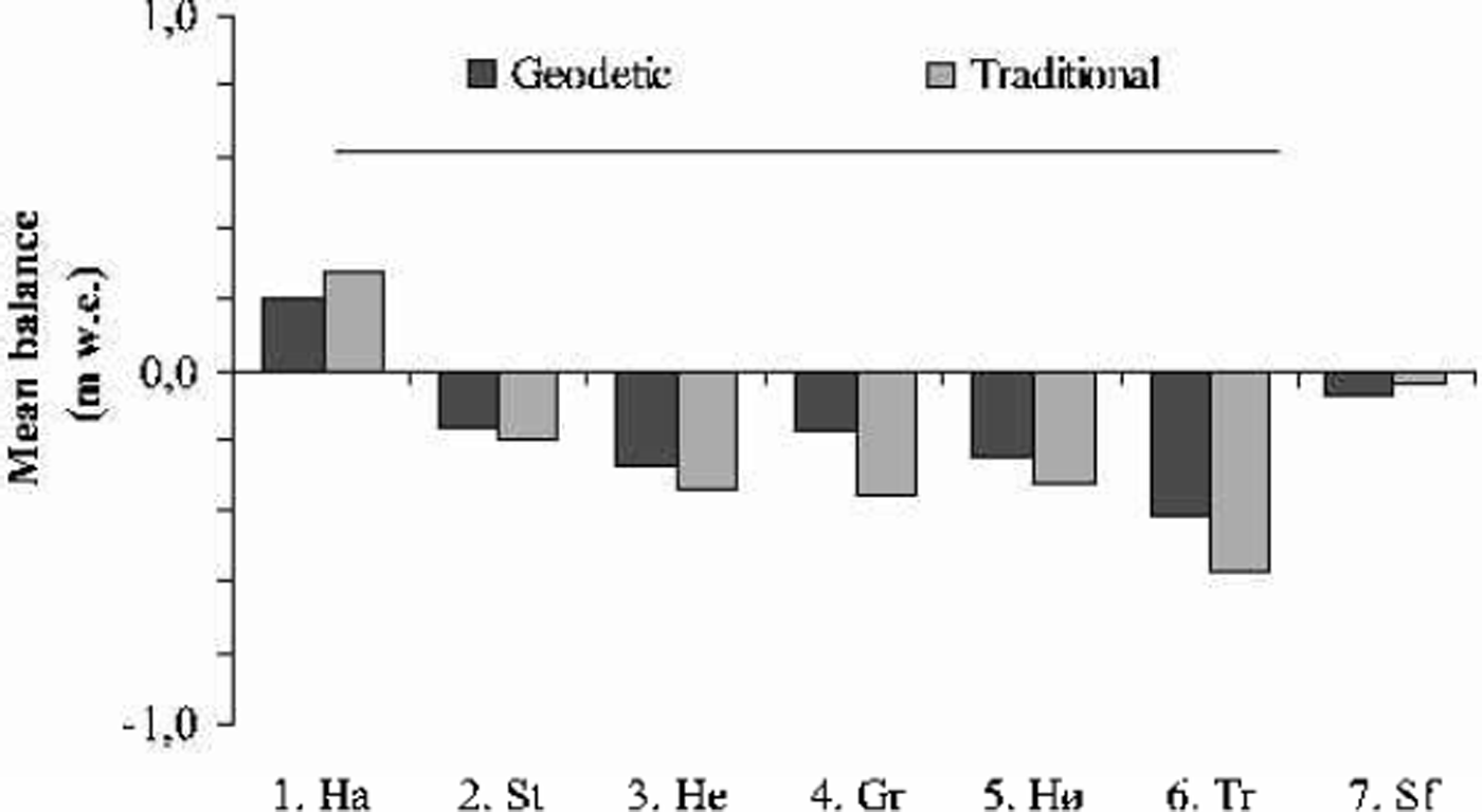
The cumulative and mean net balance results calculated from the geodetic method and from traditional mass-balance measurements are shown in Figures 2 and 3 and Table 4. Hardangerjøkulen was the only one of the investigated glaciers that experienced a significant increase in glacier volume from the 1960s to the 1990s. The geodetic and traditional methods showed net balance values of +6.8 and +9.4mw.e., respectively, for the investigated period 1961–95. All the other glaciers decreased in volume from the 1960s/70s to the 1990s. Trollbergdalsbreen had both the largest annual and total decreases in volume. The geodetic method showed a net loss of –12.3mw.e. for the period 1968–98, while the traditional and estimated measurements were more negative for this period, –16.8mw.e. The mass-balance data, other maps and aerial photos show that most of this mass loss occurred in the 1970s (Reference Andreassen, Kjøllmoen, Knudsen, Whalley and FjellangerAndreassen and others, 2000).


Table 4. Net balance results over the mapping period using the geodetic and traditional methods
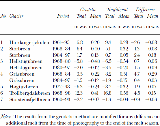
The results of the DTM comparisons were generally in agreement with the measured net balance, although there were some discrepancies. The best agreement was found for Storsteinsfjellbreen, the first measurement period on Storbreen (1968–84) and Hellstugubreen (1968–80) and the second measurement period on Gråsubreen (1984–97), where the discrepancies between the two methods were 0.4–1.3mw.e. (Table 2). These glaciers have the lowest mass turnover in this study. For the other periods and the other glaciers, larger discrepancies were found. For the first period of Gråsubreen, the discrepancy was large, but this can be explained by errors in the 1968 map (Reference HaakensenHaakensen, 1986). A new map should be made from the 1968 verticals to improve the comparison. At Hardangerjøkulen, the discrepancy of 2.6 mw.e. was acceptable and within the estimated standard error of 2.7 mw.e. for the geodetic method. The estimated error was high because of less accurate maps constructed from different control points. However, the results may also indicate that the traditional method overestimates the mass balance. The balance values in an icefall are interpolated between measurements above and below the icefall, although summer melt is greater than on the parts of a glacier with a less fractured surface (Reference Østrem and HaakensenØstrem and Haakensen, 1999). Also, for parts of the period of traditional mass-balance observations at Hardanger-jøkulen, the monitoring programme was reduced to a minimum, leading to larger uncertainties.
The discrepancies between the two methods for the three glaciers with short-term mass-balance records were not unexpected, since the traditional net balance was estimated for the bulk of the comparison period. For Høgtuvbreen and Storsteinsfjellbreen the methods differed by –0.9 and 1.9 mw.e., respectively, or –0.03 and 0.07mw.e. a–1. These results are well within the determined errors for the extrapolated traditional mass-balance data series. The largest discrepancy was 4.5mw.e., for Trollbergdalsbreen, and may be due to the uncertainty of the estimated mass balance for the years without traditional measurements. We have estimated a standard error of ±3.1mw.e. for the traditional method, compared to an error of ±1.8mw.e. for the geodetic method. However, the large volume loss showed that the glacier was not in steady state between mappings as assumed. If we use a lower density in the firn area, the geodetic net balance would be less negative, resulting in an even larger discrepancy between the methods. The DTMs of Trollbergdalsbreen are made from the same control points and are of reasonable quality, but we lack ground measurements of the glacier elevation that would confirm the accuracy of the DTMs.
For Hardangerjøkulen and Storsteinsfjellbreen, the traditional mass-balance measurements were more positive than those obtained from the geodetic method, whereas the opposite was the case for other glaciers. Thus, in most cases the geodetic method gave more positive net balance values than the traditional method, especially when the traditional results showed very negative values. However, there was no evidence in this study that one method systematically overor underestimated compared with the other. The method that gives values closest to the true net balance change cannot be determined conclusively. There are sources of errors in both methods, and each glacier must be treated separately.
Special care must be taken when interpreting results from older maps/DTMs and when comparing maps/DTMs that have been constructed from different control points. This is particularly important in the snow-covered regions of the glacier where it is difficult to map accurately. The uncertainty of the geodetic method may be reduced by better ground-control points and by ground-truth measurements of surface elevations in the snowy areas. However, fieldwork is time-consuming and expensive, and in this study we found that the advantage of the geodetic method is that it can be applied to many glaciers without involving a great deal of fieldwork and still give uncertainties within acceptable limits.
Conclusion
Glacier changes calculated by the geodetic and traditional methods have been compared for seven glaciers in Norway. Hardangerjøkulen was the only one of these investigated glaciers that experienced a significant increase in glacier volume from the 1960s to the 1990s. All the other glaciers have decreased in volume from the 1960s/70s to the 1990s. Trollbergdalsbreen had the largest annual and total decrease in volume.
The results of the geodetic method were generally in agreement with those obtained using the traditional method. The discrepancies were 0.4–4.7mw.e. The best agreements were found for Storsteinsfjellbreen and for certain measurement periods on Storbreen, Hellstugubreen and Gråsubreen. We estimated uncertainties of ±1.3–2.7mw.e. for the geodetic method, and ±1.3–3.5mw.e. for the traditional method. Ideally, if we have a pair of very high-quality DTMs of a glacier that is close to steady state between mappings, and we know the additional melt, we can obtain a standard error for the geodetic method of about ±0.7mw.e.
For five of the seven glaciers, the geodetic method gave more positive net balance values than the traditional method. However, there was no evidence that one method systematically over- or underestimated the net balance compared to the other. Which method is closest to the true net balance change cannot be determined conclusively. The uncertainties in the geodetic method can be reduced by improved ground-control points and ground-truth measurements of surface elevations. However, in this study we have applied the geodetic method to many glaciers without involving a great deal of time-consuming and expensive fieldwork, and still the uncertainties were within acceptable limits.
Acknowledgements
E. Gudevang and O. Høgberg digitized glacier maps. M. Jackson and G. Østrem read the manuscript and proposed improvements. Comments from C. Rolstad and an anonymous referee improved the manuscript.