


Introduction
The potential of Landsat-type images with high spatial resolution (<100m) to reveal surface features on terrestrial ice masses has long been recognised (e.g. Reference SwithinbankSwithinbank, 1988). Previous work has mostly been directed towards spectral classification combined with visual interpretation (e.g. Reference Orheim and LuchittaOrheim and Luchitta, 1987; Reference Dowdeswell and McIntyreDowdeswell and McIntyre, 1987). However, such analysis is hindered by the uniformity of reflectance of snow and cloud surfaces, which gives rise to a very limited range of tonal variation in such images. Texture analysis, which quantifies the spatial variation of image tone, has the potential to provide important complementary data (Reference Welch, Navar and SenguptaWelch and others, 1989, 1990; Reference KeyKey, 1990) and has already shown the value of texture analysis for identifying the presence (this is particularly difficult over snow and ice masses), and perhaps type, of cloud cover. It is not surprising that there should be considerable interest in the use of texture methods for discriminating between these image classes. Apart from the negative reason that it is difficult to effect a discrimination using only radiometric data, there is a physical justification for expecting the use of image texture to succeed, since bare ice, snow and cloud have distinct morphologies.
Techniques for the Quantification of Image Texture
It is not easy to give simple definition of image texture (Reference MatherMather, 1987; Reference ReesRees, 1990), since in principle it describes all spatial dependencies of the image. In practice, a finite number of texture parameters is defined. Typically these include the concepts of image roughness, homogeneity, linearity, contrast etc. However, the definition of these parameters often involves a subjective element so that it is possible to define a number of parameters, giving different numerical values, all of which are intended to quantify the same texture quality. Many different texture measures have been developed; the most widely used method is based on the Grey Level Co-occurrence Matrix (GLCM) (Reference Haralick, Shanmugam and DinsteinHaralick and others, 1973; Reference HaralickHaralick, 1979). In this research, we compare the performance of this method with that of a new technique, based on the concept of fractals (Reference FederFeder, 1987; Reference Lin and ReesLin and Rees, 1992), in classifying three Landsat multispectral scanner (MSS) images of the Nordaustlandet ice cap, Svalbard.
Grey Level Co-occurrence Matrix
The GLCM technique has been described in detail by Reference Haralick, Shanmugam and DinsteinHaralick and others (1973). Here we provide a summary of the important aspects.
Texture properties are defined for a two-dimensional window in the image, and calculated as various properties of the GLCM measured within the window. If the image contains n grey levels (e.g. n = 256 for 8-bit data), the GLCM is an n by n square matrix S in which the element Sij(v) is the frequency with which grey level i is separated from grey level j by a vector v. The matrix S is thus a function of the chosen displacement vector v.
Many texture parameters can be extracted from the GLCM. The three which are studied in this work are the angular second moment (ASM), the contrast (CON), and the dissimilarity (DIS)
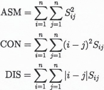
The angular second moment is essentially a measure of the homogeneity of the image, since it reaches its maximum possible value if the pixels within the image, or within the window under study, all have the same (arbitrary) grey level. It achieves its minimum possible value if the grey levels are uniformly distributed over the possible range of values, and uncorelated on the scale v used in the analysis. The contrast and dissimilarity, on the other hand, measure the tendency of neighbouring pixels to have different values of grey level, and both become zero for homogeneous images. The contrast parameter assigns a greater weight to large differences in grey level than does the dissimilarity parameter.
The angular second moment is unaffected the image calibration, but the other two paramters are changed if the calibration is changed. If the calibration is changed such that a grey level of x becomes a grey level kx, the contrast increases by a factor of k2 and the dissimiliarity by a factor of k.
In this research, the window size is chosen as 24 by 36 pixels (corresponding to an area about 2 km by 2 km on the ground), and the vector displacement v is chosen as (1,0), so that only variations in the x-direction of the image (vertically oriented features) are measured. This choice of v is clearly somewhat arbitrary, though it is quite common in the use of the GLCM for the study of image texture. In principle, one should use all possible values of v within the image window. However, the amount of computation required to generate the GLCMs and then to extract the texture paramters would be extremely large, and our result show that taking only |v| = 1 gives good discrimination of several different image classes. The restriction to vertically oriented features poses a potential problem, though for features which are likely to be statistically isotropic such as those studied in the present work the problem is likely to be more apparent than real. Again, the restriction can be justified pragmatically on the grounds that the approach yields generally good discrimination.
Fractional Brownian Motion
The fractional Brownian motion (FBM) method is based on the concept of fractals, which are geometric constructions with fractional dimensionality (as distinct from the more conventional integral dimensionality of Euclidean geometry, in which lines have dimension 1, surfaces have dimension 2, and volumes have dimension 3). The application of this idea to the study of ice sheets has been discussed in detail by Reference ReesRees (1992), who showed using Landsat imagery that the surface topography of an ice cap may be described as a surface of dimension 2.12. Since, for the purposes of the present paper, the concept of fracitional dimensionality merely provides a convenient framework in which to describe image texture, we refer the reader to the references given above, and other references contained therein, and present here only the main parameters.
The seimvariogram γ(v) of an image is defined, following (e.g.) Reference CurranCurran (1988), as
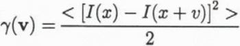
where I(x) is the grey level of the pixel whose coordinate is x, and the average represented by is performed over all the pixels lying within a window of the image. The windows were chosen to be identical to those used for the GLCM analysis. A semivariogram is formed by evaluating γ(v) for vector displacements v along a one-dimensional transect.
For surfaces which display true fractional Brownian motion,
where D is a constant known as the fractal dimension. For real surfaces this relationship is expected to break down for some minimum and some maximum value of v. The technique we adopt, described in greater detail in Lin and Rees (1992), is to plot the relationship as log (γ) against log (v) and to use an iterative procedure to define the optimum straight line through the points, and the slope of this line, from which D can be determined. We also define a parameter which we call the “shift”, which is the extrapolated value of log (γ) when log (v) = 0. It thus corresponds to the image variance for a single pixel.
Data Set
We have compared the performance of the GLCM and FBM texture methods by using them to study three Landsat MSS images of Nordaustlandet, Svalbard, for which image classifications were known. Three images were needed to give examples of all the image classes (discussed below) which we wished to study. Image 1 is band 1 (0.5 to 0.6 μm) of the Landsat 1 image from path 233, row 002, acquired on 25 March 1973. This image (which is illustrated in Reference Lin and ReesLin and Rees, 1992) shows a dry snow surface. Image 2 is band 4 (0.8 to 1.0 μm) of the Landsat 2 image from path 233, row 002, acquired on 3 July 1976. This image is partly covered by thin cirrus cloud (Fig. 1). Image 3 is band 1 of the Landsat 2 image from path 234, row 002, acquired on 1 August 1981. This image shows various melt features, as well as areas of wet snow (Fig. 2). It would have been better to be able to use the same spectral band throughout our analysis, but (a common problem with 10 or 12 year old data on magnetic tape) some channels had become corrupted. However, the very high correlation between visible and near infrared bands in images of snow and cloud means that this is unlikely to have introduced any significant errors into our study of image texture. A very simple calibration was performed on each image, by scaling the total range of grey levels to the range 0 to 63 (i.e. rescaling them to 6-bit data).
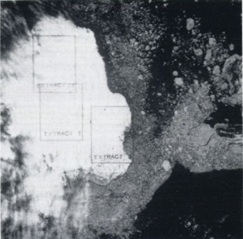
Fig .1. Image 2 (Landsat 2, Band 4, July 1876). The image shows an area approximately 185 km square.
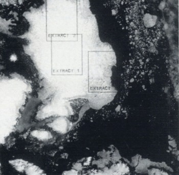
Fig .2. Image 3 (Landsat 2, Band 1, August 1981). The image shows an area approximately 185 km square.
164 windows of 24 by 36 pixels were defined within three extracts of these images, shown in Figures 1 and 2 and selected to contain areas identified as dry snow, wet snow, melt areas (distinguishable from wet snow by the appearance of melt streams and melt ponds), ablation areas, and cloud cover. These identifications were performed by visual interpretation and by comparison with Reference DowdeswellDowdeswell 1984) and G.S. Hamilton (personal communication). The texture parameters defined above were calculated for each window.
Results
GLCM technique
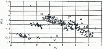
Fig .3. Principal components derived from the GLCM analysis. The circles represent dry snow, the squares wet snow, the trinagles melt areas, the lozenges ablation areas and the crosses cloud.
Values of the angular second moment (ASM), contrast (CON) and dissimilarity (DIS) were calculated for a total of 1643 windows in the three images, representing all five image classes. The results showed significant correlation between ASM, CON and DIS, and values spread over wide ranges, so a principal components analysis (e.g. Rees, 1990) was performed on the results in order to generate uncorrected texture measures. Before performing this analysis, the data were transformed to their logarithms to produce distributions which were more nearly normal.
The three principal components were found to be (ignoring additive constants)
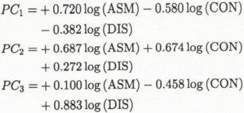
The third principal component contained less than 0.2% of the total variance and was ignored. Figure 3 shows the first two principal components, plotted as a cluster diagram. It can be seen from the figure that wet snow can be distinguished from other classes by the value of PC1, and that dry snow can be distinguished from other classes by the value of PC2. Other separations are less obvious, but we can quantify them as follows. We can define a simple index of separability S for two probability distributions p1(x) and p2(x) as
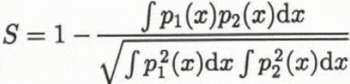
such that S = 0 if the two distributions are identical, and S = 1 if they do not overlap. Separability indices are calculated for each of the ten possible pairs of image classes, using first PC1 and then PC2, and the higher value of S is chosen. A matrix of separability values can then be defined:
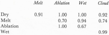
If we assume that S must be greater than about 0.8 for an effective discrimination, we can see from this table that the GLCM technique provides poor discrimination between melt areas, ablation areas and cloud cover, but that other classifications and discriminations are unambiguous.
Fractal technique
Values of the fractal dimension D and the shift parameter were calculated for 432 transects of the three images, again chosen to represent each of the five image classes. Figure 4 shows the resulting histograms for each class. It can be seen from the figure that wet and dry snow surfaces have very similar, and high, values of D. Ablation areas show somewhat smaller values of D, and melt areas and cloud cover show very broad distributions. The shift parameter is lowest for cloud, intermediate for ablation areas, and highest for wet snow, dry snow and melt areas. Separability statistics have also been calculated for the 5 classes on the basis of the distributions of D and the shift parameter, again taking the higher calculated value of S for each pair of classes, with results as follows:
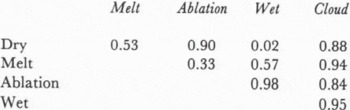
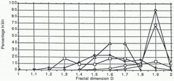
Fig .4. Histograms of the values of (a) fractal dimension D and (b) the shift parameter, from the fractional Brownian motion analysis. The symbols are as in Figure 3.
The analysis shows that the use of the fractal dimension D alone is a rather poor discriminant of image class, although with the inclusion of shift data the number of ambiguous discriminations is reduced to four, namely dry snow from wet snow and melt areas, and melt areas from ablation areas and wet snow. If the results of the FBM and GLCM separability analyses are combined, we see that the number of ambigous discriminations can be reduced to one, namely that between melt areas and ablation areas.
Discussion
Our analysis shows that the GLCM technique is, in general, able to make a more effective discrimination of image classes than is the FBM technique, although the latter achieves a greater discrimination between cloud and melt areas, and between cloud and ablation areas. However, it is less profitable to think of the techniques as rivals, but rather as complementary methods which, when combined, achieve a high level of discrimination in virtually all cases.
It is useful to compare the computational efficiencies of the two texture algorithms. For a window of size Α × Β pixels (A ≈ B), the number of operations required to calculate the GLCM Sij is approximately AB as long as the modulus of the vector v is much less than A or B. If the total number of possible grey levels is n, the number of computations required to calculate each of the three texture parameters defined in section 2 is n2. Thus the total number of operations required to generate the set of three texture parameters is approximately AB + 3n2. Taking A = 24, Β = 36 and n = 256 gives approximately 2 × 10⁵ operations. However, in practice, the range of grey levels present in Landsat images of snow, ice or cloud is very restricted, and it is more realistic to take n ≈ 10. In this case, the number of operations required to generate the GLCM parameters is closer to 103.
For a transect of length A pixels, the number of operations required to generate a semivariogram with m points is approximately mA, and the number of operations required to perform the iterative curve fitting and the extraction of the texture parameters defined in section 2 is approximately 3m2. The total number of operations required is about mA + 3m2 . Taking A = 30 and m = 12 (typical values for the size of window empoyed in this work) gives a total of about 103 operations, so that the FBM and GLCM techniques should in practice require similar amounts of computation. This was confirmed experimentally during the course of this work. However, we stress that, in principle, the calculation of GLCM-based texture measures can involve up to 100 times as much computation as the FBM measures, and that the complete classification of an image by this method could become prohibitive, requiring up to about 109 operations.
We emphasise the preliminary nature of the work described in this paper. It is open to criticism on the grounds that we have used data from several images and two spectral bands, rather than just one of each, which raises the posibility that differential calibration and sun angle effects may affect our results. It must also be stressed that the use of texture analysis in image classification should not be relied upon until the physical mechanisms responsible for generating the image texture are clearly understood. At present this can be done only in a very broad and qualitative way by recognizing that different surface morphologies will give rise to different image textures, but we are currently attempting to put this understanding on a quantitative basis. For example, the high value of the fractal dimension D measured for wet and dry snow areas can be understood since in these areas variations in image brightness are likely to be caused predominantly by topographic variation (Reference Rees and DowdeswellRees and Dowdeswell, 1988), and this is small in the areas studied (Reference Dowdeswell and McIntyreDowdeswell and McIntyre, 1987). Lower values of D for melt areas probably reflect real variations in the surface structure at scales of less than the image window size of 2 km. If an understanding at this level can be quantified and extended to include the GLCM parameters, it should allow questions such as the optimum spatial resolution and window size, and the optimum spectral band (or combination of bands) to be determined. However, we believe that the general conclusion from this work will continue to stand, namely that the use of texture techniques (probably a combination of GLCM and fractal techniques) has the potential to provide unambiguous classifications of images of snow, ice and cloud, and that this classification can ultimately be automated.
Conclusions
We have applied two texture measures to three temporally separated Landsat MSS images of the Nordaustlandet ice cap. The results show that different image classes have distinct textures, and confirm that texture analysis provides powerful additional information for the classification of such images. The results show that the use of the three GLCM texture parameters (angular second moment, contrast and dissimilarity) gives in most cases greater discrimination of surface classes than the use of the fractional Brownian motion technique. However, the two techniques appear to have different strengths and weaknesses, and their combination yields a high level of discrimination of all the image classes studied.
Acknowledgements
We gratefully acknowledge the technical assistance of Drs B.J. Devereux and J. A. Dowdeswell, and of Messrs O. Dikshit, M. R. Gorman, T. Mayo and G. Hamilton. The comments of Drs R. Bindschadler and R. A. Massom, and of an anonymous referee, have greatly improved the presentation of this work.


