


INTRODUCTION
The subglacial environment exerts a substantial control over the flow dynamics of glaciers and ice masses (Bell, Reference Bell2008; Siegert and others, Reference Siegert2018). A major uncertainty in ice dynamic models is the limited understanding of processes at the ice/bed interface and the composition of subglacial material. A significant control on ice motion is whether ice is underlain by the hard or soft substrate, and therefore whether the motion is governed by ice/sediment deformation (Hofstede and others, Reference Hofstede2018) or sliding (Stearns and van der Veen, Reference Stearns and Van der Veen2018). Such compositional variations are typically parameterised in predictive models by assuming a frictional stress coefficient (Christoffersen and others, Reference Christoffersen, Bougamont, Carter, Fricker and Tulaczyk2014; Åkesson and others, Reference Åkesson, Nisancioglu, Giesen and Morlighem2017), although recent work by Stearns and Van der Veen (Reference Stearns and Van der Veen2018) highlights the potentially greater influence of effective basal pressure. Where underlain by sediment, the hydrological properties of the subglacial environment, therefore, have a profound effect on glacial flow and require proper consideration in ice dynamic modelling (Kulessa and others, Reference Kulessa2017; Siegert and others, Reference Siegert2018).
Quantitative geophysical analysis of subglacial material is typically not straightforward: although many geophysical methods can assess the mechanical properties of glaciers and ice masses, they can be problematic for characterising material much beyond the immediate vicinity (~2 m) of the glacier bed (Booth and others, Reference Booth2012). Seismic reflection methods often lack the resolution or signal-to-noise ratio for quantifying subglacial material properties and, for example, may be limited to amplitude-versus-offset (AVO) studies of basal reflectivity (e.g., Anandakrishnan, Reference Anandakrishnan2003; Booth and others, Reference Booth2012; Kulessa and others, Reference Kulessa2017). Seismic refraction methods are limited by their low depth penetration into subglacial material (e.g., Thiel and Ostenso, Reference Thiel and Ostenso1961; Bentley and Kohnen, Reference Bentley and Kohnen1976; King and Jarvis, Reference King and Jarvis2007); refraction interpretations are impeded since an ice/sediment interface typically represents a velocity reduction, hence critical refraction will not occur and a head-wave will not be generated. Ground penetrating radar (GPR) methods are well suited to characterising englacial properties (e.g., Murray and others, Reference Murray, Booth and Rippin2007; Young Kim and others, Reference Young Kim2010; Booth and others, Reference Booth2013; Lindbäck and others, Reference Lindbäck2018), but glacier bed reflectivity and high attenuation within the ice column limits the utility of subglacial radar sampling.
Dispersion curve analysis of surface (Rayleigh) waves presents an alternative method for characterising seismic properties of basal material, for both passive- or active-sources, by constraining the variation of shear wave velocity (Vs) with depth (Xia and others, Reference Xia, Miller, Park and Tian2003). Rayleigh waves are a form of seismic wave that travel along the ground-surface, termed ‘groundroll’ in reflection seismology and although often considered as noise, they contain ~2/3 of the total energy of a typical surface source (Richart and others, Reference Richart, Hall and Woods1970). In passive seismology, Picotti and others (Reference Picotti, Francese, Giorgi, Pettenati and Carcione2017) used the horizontal-to-vertical spectral ratio (HVSR) technique to map glacier and ice-sheet thicknesses and, in certain conditions, obtain reliable estimates of the basal seismic properties. Preiswerk and Walter (Reference Preiswerk and Walter2018) used high frequency (>2 Hz) ambient seismic noise, collected on alpine glaciers, to estimate ice thickness and infer potential bed properties. These techniques are analogous to those used to determine the properties of the Earth's deep interior (Shen and others, Reference Shen2018). Within active seismology, the use of Rayleigh wave dispersion curves is termed ‘Multichannel Analysis of Surface Waves’ (MASW).
Regardless of the source of the dispersion curve, characterising Vs offers a promising means of distinguishing material within the subglacial environment, since shear wave properties vary with rigidity (shear modulus). Various researchers have used Vs to distinguish between hard and soft glacier substrates (Picotti and others, Reference Picotti, Vuan, Carcione, Horgan and Anandakrishnan2015), or the boundary between frozen and unfrozen zones within sediment (Tsuji and others, Reference Tsuji, Johansen, Ruud, Ikeda and Matsuoka2012). Zimmerman and King (Reference Zimmerman and King1986) showed that seismic velocities vary significantly with the degree of pore-fluid freezing, with Vs increasing by as much as 90% as pore water freezes (Johansen and others, Reference Johansen, Digranes, Van Schaack and Lønne2003). Current applications of MASW methods within cryosphere studies include: identifying Vs and density structure within firn (Armstrong, Reference Armstrong2009; Diez and others, Reference Diez2014), identifying velocity (Vs) structure within shallow ice (Tsoflias and others, Reference Tsoflias, Ivanov, Anandakrishnan and Miller2008b; Young Kim and others, Reference Young Kim2010), monitoring and mapping embedded low Vs zones in permafrost areas (Dou and Ajo-Franklin, Reference Dou and Ajo-Franklin2014) and identifying unfrozen zones in subglacial sediments (Tsuji and others, Reference Tsuji, Johansen, Ruud, Ikeda and Matsuoka2012).
However, Vs depth profiles obtained from MASW suffer from poor depth resolution (Foti and others, Reference Foti2015). Even for the active-source case, using frequencies that are typically higher than for passive seismology, vertical resolution can be limited to ~10 m. Indeed, at a fundamental level, the inversion of dispersion curves is also nonunique: many profiles of Vs (spanning a disparate set of physical structures) may be consistent with the observed data within the error tolerance. These limitations can be mitigated by constraining the MASW inversion using independent and complementary information, in our case the high-resolution determination of internal horizons using co-located GPR surveys, which vastly reduces the space of acceptable models with an associated marked increase in vertical resolution. Key to this method is that the relevant subsurface horizons (e.g., the snow ice surface and the glacier bed) represent contrasts in both electromagnetic and elastic properties.
A recently developed method for depth-constrained MASW inversion, MuLTI (Multimodal Layered Transdimensional Inversion; Killingbeck and others, Reference Killingbeck, Livermore, Booth and West2018) is applied in this paper to characterise the subglacial environment. We invert surface wave dispersion curves to evaluate the variation of Vs with depth and assess its accuracy and uncertainty. Following a synthetic study, we analyse a combined MASW-GPR dataset acquired using an active source on Midtdalsbreen, an outlet glacier of Norway's Hardangerjøkulen ice cap. Although applied here to active-source data, the seismic data enters MuLTI only through a dispersion curve, implying that MuLTI is equally valuable as a tool for passive-source seismology with associated depth constraints (which can be from any independent source: e.g., airborne radar or borehole control). Thus, MuLTI is a novel methodology for investigating the subglacial environment for a range of glacier settings and seismic data types.
METHOD
Multichannel analysis of surface waves
MASW surveys use an array of geophones in-line with an active seismic source located on the ground-surface, similar to the acquisition performed for a 2-D seismic reflection survey. The original field records, in the time-space domain, are transformed into the frequency-wavenumber domain, where the dispersive pattern of the Rayleigh waves can be determined by picking the spectral maximum (Park and others, Reference Park, Miller and Xia1998).
The above process requires the following detailed steps. Dispersion curves are calculated from the seismic data using common midpoint cross-correlation (CMPCC) gathers (Hayashi and Suzuki, Reference Hayashi and Suzuki2004) and the MASW method introduced by Park and others (Reference Park, Miller and Xia1999). CMPCC gathers are created by cross-correlating every pair of traces in each shot gather before sorting into CMP gathers. In each CMP gather, the equally spaced traces were stacked in the time domain to yield CMPCC gathers. To image dispersion curves in the phase velocity-frequency domain, phases of the cross-correlated data were shifted and stacked in the frequency domain, as described in Park and others (Reference Park, Miller and Xia1999).
The dispersion curve depends upon the near-surface elastic properties (compressional wave velocity (Vp), Vs and density), assumed horizontally homogeneous beneath the geophone spread, although with the strongest sensitivity to Vs (Xia and others, Reference Xia, Miller, Park and Tian2003). The frequency range over which phase velocity is considered reliable corresponds to the minimum and maximum wavelengths recorded. For any given frequency (f), the wavelength (λ) is specified as
 $$\lambda _\; = \displaystyle{{PV(\,f)} \over f}$$
where PV is the phase velocity of any frequency component (Stokoe and others, Reference Stokoe, Wright, James and Jose1994). The resolvable scale of a given frequency component, L, is ~λ/3 (Gazetas, Reference Gazetas1982), implying that the finite bandwidth f min to f max is associated with a range of resolution from L max ≥ L ≥ L min, where L min is the thinnest resolvable layer and L max is the maximum resolvable depth. This maximum depth is considered conservative, as other researchers (e.g., Park and others, Reference Park, Miller and Xia1999; Tsuji and others, Reference Tsuji, Johansen, Ruud, Ikeda and Matsuoka2012) base this estimate on a λ/2 approximation. However, MuLTI incorporates additional independent depth constraints (elaborated in the next section) which widen these bounds and improves the resolution beyond what is possible with surface waves alone (Killingbeck and others, Reference Killingbeck, Livermore, Booth and West2018). The useful bandwidth of the survey depends on the signal-to-noise ratio in the dataset, the frequency output of the source, and the length of the survey line. A long survey line is favourable for long wavelengths and hence large L max, but this risks invalidating the assumption of horizontal homogeneity; furthermore, lateral resolution is governed by the range of offsets in each CMPCC gather, hence longer offsets imply greater smearing of horizontal structure (Park, Reference Park2005). However, the resolution of dispersion curves improves as the ratio of wavelength to source-receiver offset increases; hence, for any fixed geophone spread, the low frequencies have a poorer resolution in the dispersion image and their interpretation is less precise (Park and others, Reference Park, Miller and Xia2001).
In layered media, inversion for subsurface structure is complicated by the fact that the observed dispersion curve is the combined effect of the different modes of propagation (Foti and others, Reference Foti2015), ultimately filtered by the physical survey itself which depends upon the survey design parameters. To ensure a good fit, models need to account for not only the fundamental mode (Park and others, Reference Park, Miller and Xia1999) but all its higher-order harmonics, referred to as ‘modes’ of propagation. Early models of surface wave inversion only considered the fundamental mode with simple near-surface environments (Xia and others, Reference Xia, Miller and Park1999). However, higher order modes have shown to dominate in several types of velocity structures, for example when a high-velocity layer overlays a low-velocity layer (Gucunski and Woods, Reference Gucunski and Woods1992). Therefore multimodal analysis of surface waves is important when anticipating these complex velocity profiles. Our MuLTI algorithm is compatible with such multimodal inversions.
MuLTI
MuLTI is a Bayesian inversion method that seeks to determine the posterior distribution of Vs, as a function of depth, for a prescribed profile of Vp and density, which is fully described in Killingbeck and others (Reference Killingbeck, Livermore, Booth and West2018). The method does not require the number of subsurface layers to be fixed but rather, in a ‘transdimensional’ framework, allows the data to self-determine the required complexity of the distribution (e.g., Bodin and Sambridge, Reference Bodin and Sambridge2009; Bodin and others, Reference Bodin2012; Livermore and others, Reference Livermore, Fournier, Gallet and Bodin2018). Its particular utility here is the ability to include subsurface depth constraints, mitigating poor resolution and nonuniqueness of inversions from surface wave dispersion curves alone.
MuLTI is initiated with frequency-phase velocity picks of Rayleigh wave dispersion curves, together with a measure of their uncertainty derived from the half width of the dispersion curve. The depth constraints determined here from GPR data fix particular layer boundaries in the inversion, a self-consistent procedure as the GPR-derived depths are accurate to the decimeter scale: about a factor of 100 more accurate than the sensitivity of the Rayleigh waves.
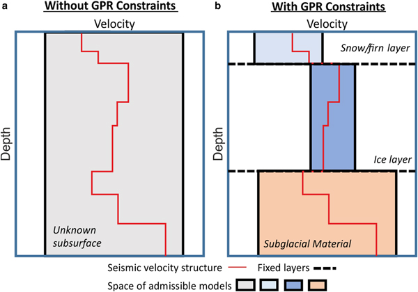
Figure 1 illustrates MuLTI's model geometry and shows schematic differences between the unconstrained (Fig. 1a) and depth-constrained (Fig. 1b) cases. If no depth constraints of the subsurface interfaces are available, the unconstrained substructure is characterised (before the introduction of seismic data) by wide bounds on Vs (e.g., Vs between ~200 and 2800 m s−1). However, when using co-located GPR data, layer boundaries (e.g., snow/ice) can be identified and the constraints on Vs can be tightened assuming each layer can be attributed to a known material. For example, in this paper, we assume that the upper two layers within the glacier are snow and ice, each with known depth and assumed Vs range (500–1700 m s−1 for the snow layer and 1700–1950 m s−1 for the ice layer), thus significantly reducing the model parameter space.
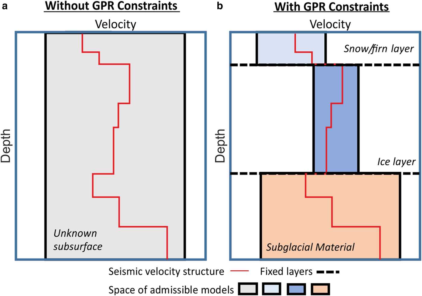
Fig. 1. Illustration of MuLTI's model parameterisation comparing (a) a 1-layer model with no internal layers and (b) a GPR-determined three-layer structure assuming different ranges of Vs within each layer. Shaded boxes indicate the range of possible Vs values. Figure adapted from Killingbeck and others (Reference Killingbeck, Livermore, Booth and West2018).
MuLTI uses the Geopsy theoretical modal dispersion curve algorithm of Wathelet and others (Reference Wathelet, Jongmans and Ohrnberger2004), Wathelet (Reference Wathelet2005) as a forward model to compare any proposed substructure model to the observed data (picked Rayleigh wave dispersion curve). It numerically approximates the posterior distribution by an ensemble of models (a Markov chain), traversing the space of admissible models (shaded boxes shown in Fig. 1), sampling the models with greater likelihood more often. Provided the ensemble size is large enough, the statistics of the ensemble will converge to those of the underlying posterior distribution. MuLTI produces a variety of diagnostic statistics of the Vs ensemble that can be analysed to quantify uncertainty in the subsurface properties. In our analysis, we mainly use the mode and average Vs profiles to visualize our preferred structure, along with the 95% credible interval as an estimate of uncertainty.
FIELD SITE: MIDTDALSBREEN
Midtdalsbreen, 6.8 km2 in area, is a NE-flowing outlet glacier of the Hardangerjøkulen ice cap in central-southern Norway (60.59°N, 7.52°E; Fig. 2). Hardangerjøkulen is Norway's 6th largest glacier (71.28 km2) (Andreassen and Winsvold, Reference Andreassen and Winsvold2012) and is an important water source for local river catchments. Annual glacier length measurements performed by A. Nesje between 1982 and 2018 show that the front of Midtdalsbreen advanced 36 m between 1982 and 2001, but retreated 219 m between 2001 and 2018 (e.g., nve.no/hydrologi/bre; Reinardy and others, Reference Reinardy2019), thus exposing material recently melted out from beneath the glacier. At the time of acquisition, April–May 2018, the subsurface comprised snow (~2–4 m thick) overlying a varying thickness (0–25 m) of glacier ice and a substrate of unknown subglacial material. Midtdalsbreen is well-suited to methodological development since it is both logistically accessible and has a simple wedge-shaped profile (Fig. 3), which is valuable for this study since ice thicknesses show little cross-glacier variation.
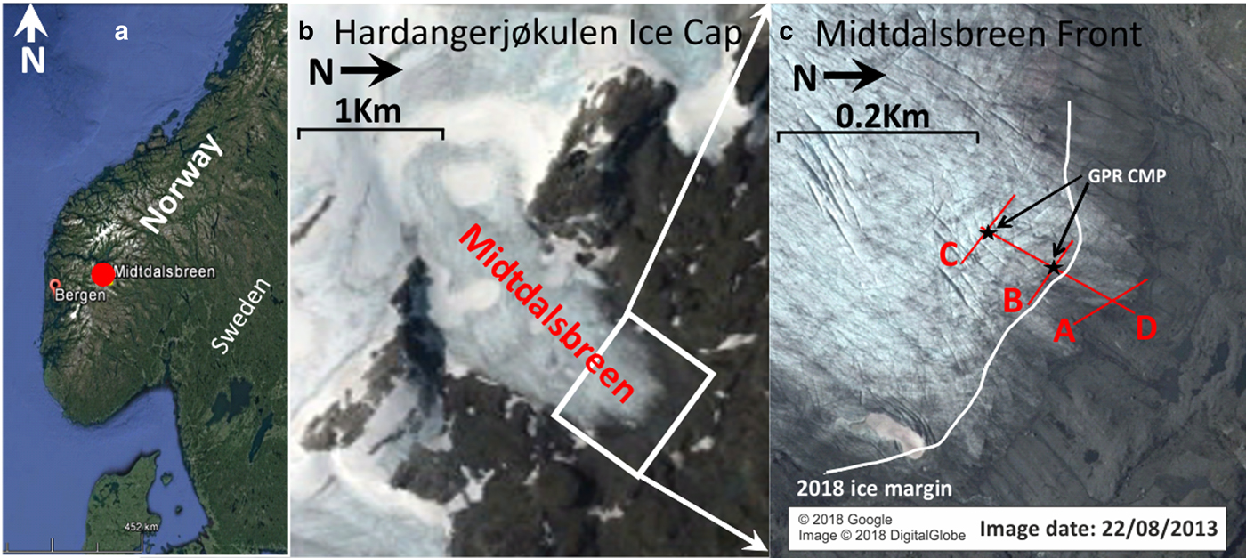
Fig. 2. (a) Location of Hardangerjøkulen ice cap, South Norway. (b) Google Earth image of Midtdalsbreen, an outlet glacier of the Hardangerjøkulen ice cap. (c) Survey lines acquired during the 2018 field season at the front of Midtdalsbreen. Google Earth satellite images taken in 2013. Note that (b) and (c) are orientated away from north to enable optimal data comparison in later figures.
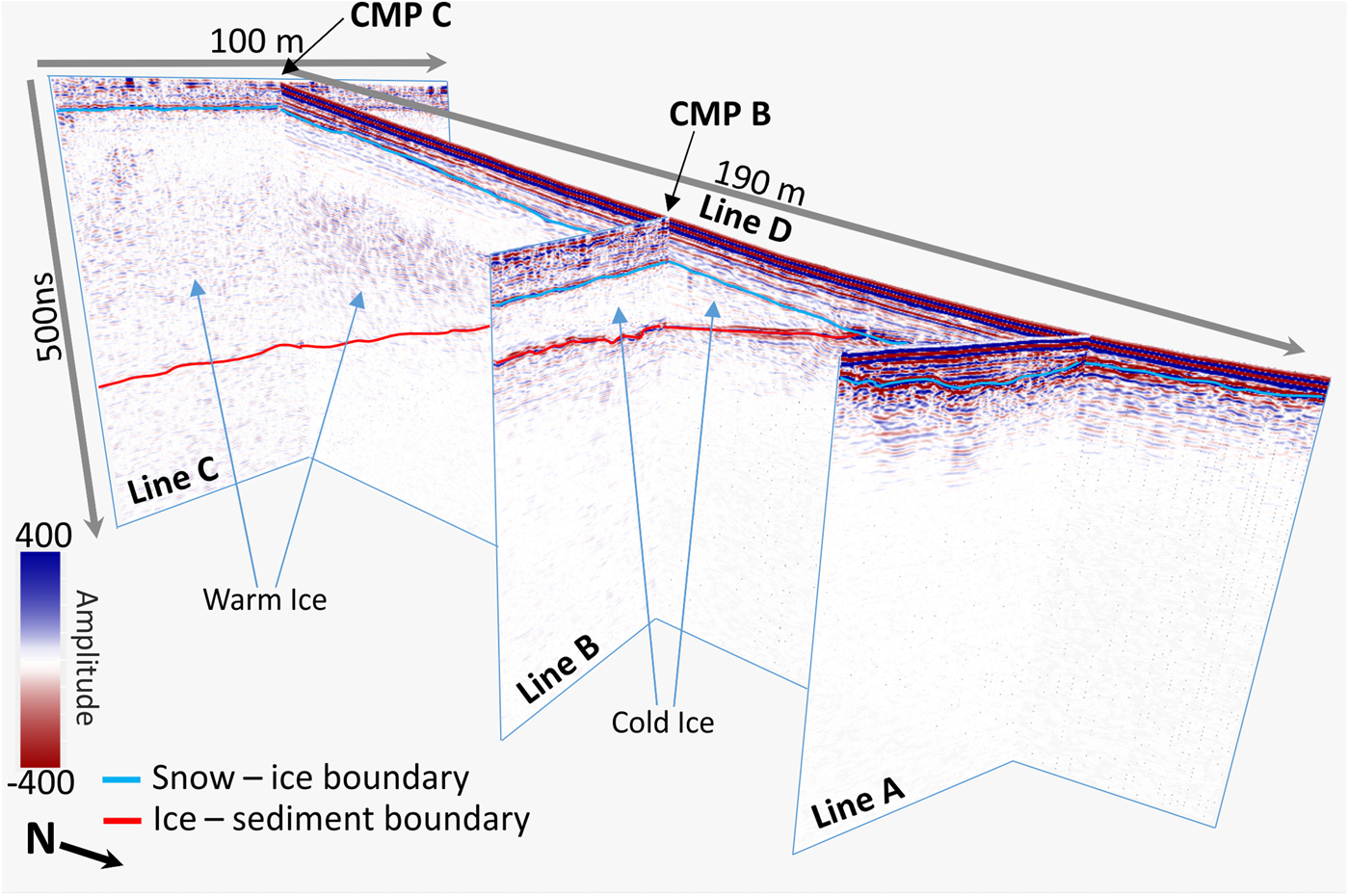
Fig. 3. GPR lines acquired at the front of Midtdalsbreen directly along the 2-D seismic survey lines: A, B, C and D. Snow (blue) and ice (red) horizons were picked in two-way traveltime (TWT).
Previous GPR data acquisitions show the glacier to have a 40 m wide cold-ice zone within the majority of the glacier tongue, where ice thickness is <10 m (Reinardy and others, Reference Reinardy2019). The glacier thickens beyond its tongue and primarily consists of warm ice within the ablation area surveyed in this study. Midtdalsbreen is surrounded by mountains of phyllite and crystalline granite and gneiss. Little Ice Age marginal moraines (post-1750 CE) on the glacier foreland primarily consist of subglacial traction till with both granite, gneiss and phyllite clasts indicating the glacier has a debris-rich basal ice layer probably underlain by sediments and areas of eroded subglacial bedrock (Reinardy and others, Reference Reinardy, Leighton and Marx2013).
Several studies have inferred subglacial erosion, transport and depositional processes at Midtdalsbreen from sedimentological and geomorphological observations made in the foreland (Andersen and Sollid, Reference Andersen and Sollid1971; Etzelmüller and Hagen, Reference Etzelmüller, Hagen, Harris and Murton2005; Reinardy and others, Reference Reinardy, Leighton and Marx2013, Reference Reinardy2019; Willis and others, Reference Willis, Fitzsimmons, Melvold, Andreassen and Giesen2012). Repeated observations indicate >50 cm thick sequences of highly saturated till, clay to silt-rich deposits linked to ponding meltwater, and comparatively lower volumes of sand/gravel meltwater stream deposits along with highly polished and striated phyllite. Directly in front of the glacier, end moraines and flutes are occasionally ice-cored while some till-covered areas of the foreland may also be underlain by dead-ice (ice disconnected from the glacier). However, the distribution of sediments can be highly variable, in both space and time, given the melting of ice cores and the erosion and reworking of sediment by meltwater (Reinardy and others, Reference Reinardy, Leighton and Marx2013; Reference Reinardy2019). The general lower limit of permafrost in this area is estimated to be 1550 m a.s.l., however DC-resistivity soundings at 1450 m a.s.l. and thermistor measurements of cold-ice (<0°C) at the glacier front of Midtdalsbreen indicate permafrost at lower elevations (Etzelmüller and others, Reference Etzelmüller, Berthling and Sollid2003).
To explore the subglacial extent of sediment, Willis and others (Reference Willis, Fitzsimmons, Melvold, Andreassen and Giesen2012) investigated the Midtdalsbreen's subglacial drainage system using dye tracing methods. They suggested that the glacier has a split drainage system, with a hydraulically efficient distributed system on the eastern section and an inefficient linked cavity system on the central and western sections. In addition to demonstrating the performance of the MuLTI algorithm, we anticipate that our results will offer additional insight into sediment and ice flow characteristics at the site.
DATA ACQUISITION
Seismic acquisitions were performed around and over the glacier front (Fig. 2c) with a Geometrics GEODE system and 48 10 Hz vertical-component geophones. For cross-glacier lines A, B and C, the source and geophone locations had 2 m intervals; for the down-glacier line D, these were increased to 4 m. GPR profiles were acquired along the length of the seismic lines with Sensors & Software PulseEKKO PRO unshielded 200 MHz antennas. Figure 3 displays the processed GPR lines and the interpreted position of snow ice and ice-bed horizons. These horizons are generally well defined and can be picked with confidence, although the signal-to-noise ratio at the glacier bed is low below the cold-warm transition surface (where the ice is >20 m thick).
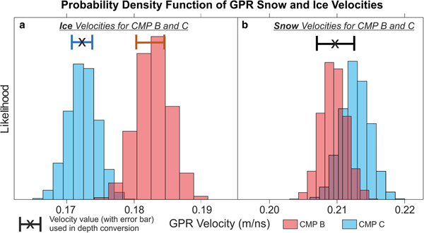
The thickness of snow and ice layers was estimated from velocity analysis of GPR common midpoint gathers (CMP) located half way along the seismic spreads B and C (Booth and others, Reference Booth, Clark and Murray2011). Figure 4 shows CMP gathers B and C with their associated semblance responses, also marking the picked velocities and their corresponding reflection hyperbolae following velocity corrections using the method described in Booth and others (Reference Booth, Clark and Murray2010). GPR velocities and their uncertainties are expressed as probability density functions in Figure 5, using a Monte Carlo method (Booth and others, Reference Booth, Clark and Murray2011). For the snow layer (Fig. 5b), the CMP analyses yielded a similar median, hence a single average interval velocity (0.2100 ± 0.0029 m ns−1) is assumed in-depth conversions. For the ice layer (Fig. 5a), analysis from CMP B and CMP C determines differing velocities by ~6%, possibly related to the greater englacial water content at CMP C and therefore more intense scattering at this site. However, the velocity estimate from CMP C (0.1724 ± 0.0015 m ns−1) is more consistent with cold ice from other locations (Murray and others, Reference Murray, Booth and Rippin2007; Saintenoy and others, Reference Saintenoy2013; Temminghoff and others, Reference Temminghoff, Benn, Gulley and Sevestre2018) hence this value is used to evaluate ice thickness.
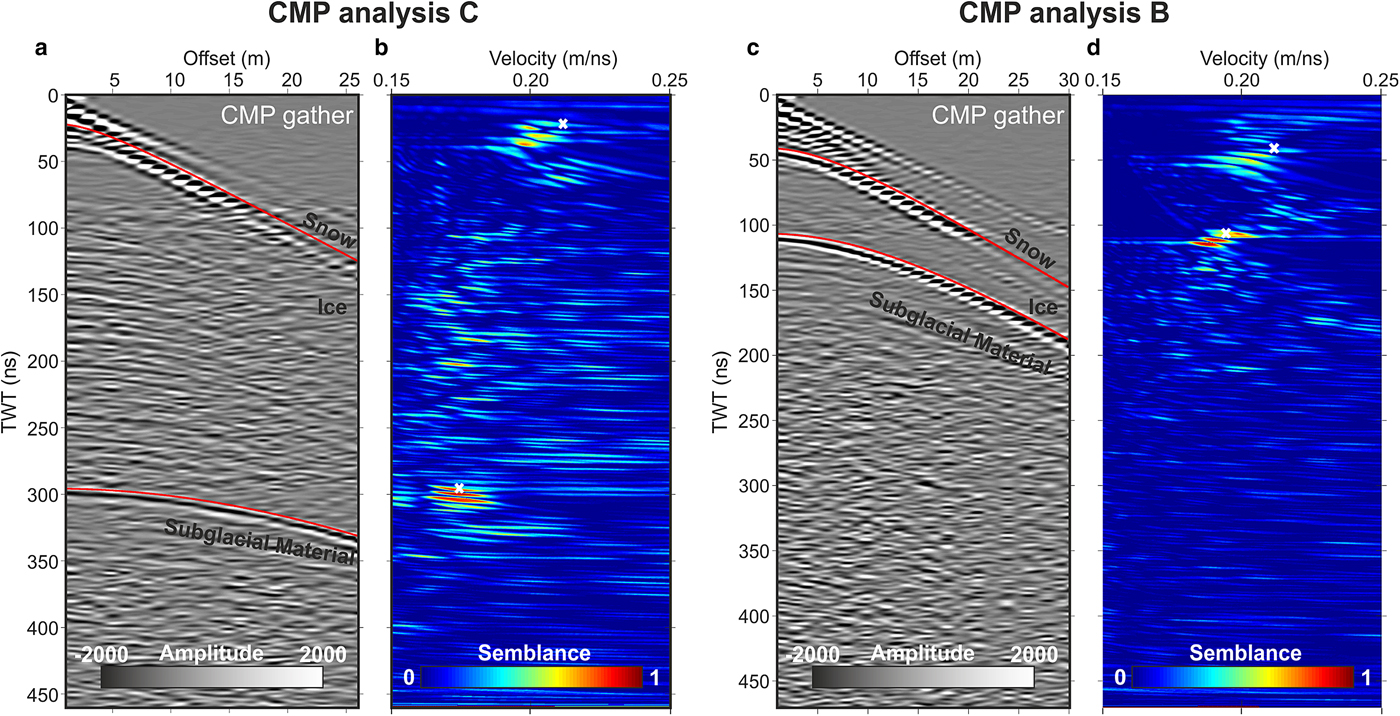
Fig. 4. GPR CMP gathers acquired at the midpoint of lines B and C with corresponding semblance plots in two-way traveltime (TWT). (a) CMP analysis for the midpoint of line C and (b) CMP analysis for midpoint of line B. Picked velocities are highlighted by the white ‘X’ and their corresponding hyperbolae are shown in red (Booth and others, Reference Booth, Clark and Murray2010).

Fig. 5. GPR velocity precision results, using Booth and others (Reference Booth, Clark and Murray2011) Monte Carlo simulation method, displaying probability density functions of (a) ice and (b) snow GPR velocities derived from CMP B and C.
SYNTHETIC STUDY
A synthetic study was conducted to validate MuLTI based on a likely target subsurface and to determine inversion parameters for the acquired data. Various 1-D-block models, shown in Fig. 6; a–d (note a–d are unrelated to the seismic lines denoted A–D) were created to represent different glacial and subglacial environments which may be expected at Midtdalsbreen glacier, including snow, glacier ice, water saturated till (low Vs zone) and bedrock. Each layer was populated with Vp, Vs and density values representative of each layer (Fig. 6), obtained from example glaciological seismic studies (Peters and others, Reference Peters2008; Tsoflias and others, Reference Tsoflias2008a; Podolskiy and Walter, Reference Podolskiy and Walter2016). Inversion parameters are documented in Table S1 in the supplementary material and explained fully in Killingbeck and others (Reference Killingbeck, Livermore, Booth and West2018).
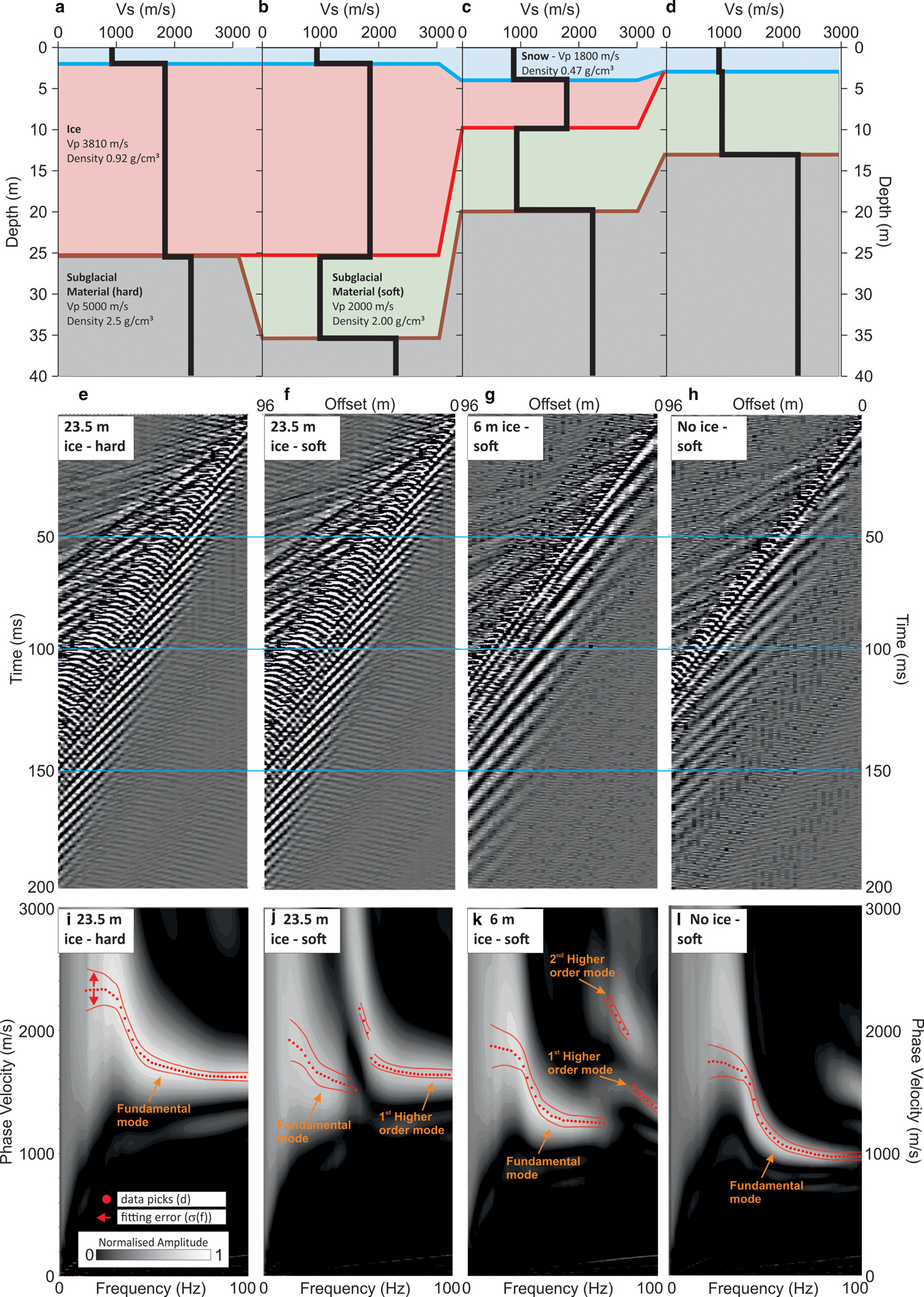
Fig. 6. 1-D block models created to simulate snow and ice thicknesses expected at Lines A, B and C (a–d). Blue, red and brown lines represent base snow, ice and soft substrate boundaries; DWM synthetic wavefield shot gathers (e–h); corresponding dispersion curves picked with an estimate of associated uncertainty derived from the width of the dispersion image (i–l).
Synthetic waveforms were calculated from the 1-D block models using the Discrete Wavenumber Method (DWM) (Bouchon and Aki, Reference Bouchon and Aki1977). This calculates the full waveform, which can be considered an analogue of the observed data in terms of phase velocity and amplitude (Figs 6e–h). The DWM parameters used to calculate the synthetic waveforms are the same as those used for the acquisition of our cross-glacier lines: 48 geophones with 2 m spacing. The maximum amplitudes of the frequency-phase velocity images were picked to create the Rayleigh wave dispersion curves which were used as input to MuLTI together with an estimate of their uncertainty, σ(f), approximated from the half width of the peak, in velocity, at each given frequency (red lines in Figs 6i–l); this is seen to decrease with increasing frequency. The synthetic dispersion images clearly display a fundamental mode along with first and second higher order modes (higher order modes being induced by the low-velocity layer immediately underlying the high-velocity ice). Comparing reference models (Figs 6i and l), with increasing velocity structure, to the complex velocity models (Figs 6j and k), shows that the presence of a sharp decrease in velocity causes a break in the fundamental mode and higher order modes become more dominant. The depth of the velocity change is directly related to the frequency at which the change in dominant mode (from fundamental to higher order) occurs.
The resolution of the dispersion curve, and the precision with which its maxima can be picked is influenced by survey parameters. Longer source-receiver offsets sharpen the dispersion curve and clarify the transition between different modes. However, long offsets in real data become dominated by body waves (e.g., reflections and refractions) hence there is a compromise between dispersion resolution and signal-to-noise ratio (Park and others, Reference Park, Miller and Xia2001; Park, Reference Park2005). This issue becomes evident in our real data and is considered in our discussion section.
In this synthetic example, picking of dispersion curves is restricted to frequencies of 14–100 Hz, representative of the bandwidth in our real data. Killingbeck and others (Reference Killingbeck, Livermore, Booth and West2018) show that including higher frequencies (>100 Hz) causes instabilities related to the appearance of higher-order modes hence we deliberately omit them in our analysis. Using Eqn (1) and the λ/3 wavelength sampling approximation (Gazetas, Reference Gazetas1982), the dispersion curves picked in these examples have a thinnest resolvable layer (L min) of 3 m (corresponding to no ice model, Fig. 6d), 4.5 m (6 m ice model) and 5.6 m (23.5 m ice models); and maximum resolvable depth (L max) of 30 m (no ice model), 45 m (6 m ice model) and 46 m (23.5 m ice models).
The inversions were run using Vs boundaries, and corresponding Vp and density values, set to the parameters stated in Table 1. Tests on varying Vp and density on modal dispersion curves show small variations but these are mostly within the fitting error tolerance (σ) used in MuLTI, Figure S1 in the supplementary material. Given the maximum resolvable depth of 46 m (from purely surface wave data), inversions were performed for a maximum depth of 40 m. To highlight the benefit of additional depth constraints (e.g., derived from GPR), MuLTI is first run for an unconstrained case and thereafter with fixed depths of the snow ice and ice-bed layers. One million iterations were run and found to be sufficient for convergence of the posterior distribution sampled; more detailed inversion parameters used are documented in Table S1 in the supplementary material and explained further in Killingbeck and others (Reference Killingbeck, Livermore, Booth and West2018).
Table 1. Elastic parameter boundaries applied in MuLTI for the glacier feasibility study. The parameters are taken from Peters and others (Reference Peters2008); Tsoflias and others (Reference Tsoflias2008a); Podolskiy and Walter (Reference Podolskiy and Walter2016)
Posterior Vs distributions produced from MuLTI are shown in Figure 7. The probability density distribution of Vs profiles within their 95% credible interval is plotted as coloured contours alongside the true solution (black line). The highest density distribution (red) for each depth corresponds to the most likely Vs model. The unconstrained inversions in Figures 7a–c show significant deviation between the true model and inversion output, with respective depth-averaged Vs errors of 680 m s−1, 1046 m s−1 and 567 m s−1, respectively, based on the modal model; although the fit is better (240 m s−1 error) for 7d (and 7a in the ice layer only), given the simpler underlying parameter distribution, there are multiple Vs distribution peaks between 20 and 33 m. The addition of depth constraints improves the match throughout, and Figures 7e–h show errors of 256 m s−1, 99 m s−1, 164 m s−1 and 138 m s−1, respectively (factors of 2.7, 10, 3.5 and 2 improved on their unconstrained equivalents).
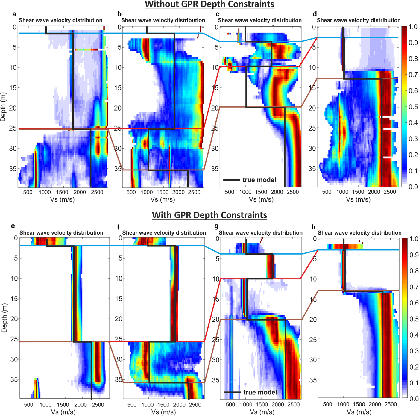
Fig. 7. Posterior Vs distributions determined from MuLTI inversion (a–d) without depth constraints and (e–h) with depth constraints; the models correspond to those shown in Fig. 6a–d. Colour scale represents the probability density distribution of Vs values within the 95% credible interval, red highlighting most likely. Black line shows the true synthetic Vs profiles. Blue, red and brown correlation lines highlight the snow, ice and soft substrate depths respectively.
More complex synthetic modelling, including an additional ice debris layer (high Vs) at the base of the glacier which may not be detected by GPR data, shows MuLTI can reliably resolve unconstrained layers not accounted for in the GPR depth constraints applied within MuLTI (Figure S2 and S3 in the supplementary material).
This feasibility study demonstrates MuLTI works well for the expected geometries and parameter distributions for the Midtdalsbreen dataset. It also highlights the significant added value of depth constraint when a complex velocity profile is expected.
RESULTS
1-D shear wave velocity profiles
We first produced 1-D velocity profiles for CMPCC gathers (Hayashi and Suzuki, Reference Hayashi and Suzuki2004) located at the centre of lines A, B and C (Fig. 8). A different range of source-receiver offsets was used in each gather due to differences in data quality and subsurface complexity. This minimises the spatial averaging affect beneath the geophone spread, particularly where the subsurface is not horizontally homogeneous (Park, Reference Park2005). Line A shows significant interference between Rayleigh and body waves for offsets >50 m, whereas co-located GPR data suggest that the subsurface can only be described as 1-D for offsets <60 m at Line B. However, data from Line C suffers from no such restrictions, hence its CMPCC gather uses the full 92 m offset range for this 1-D analysis.
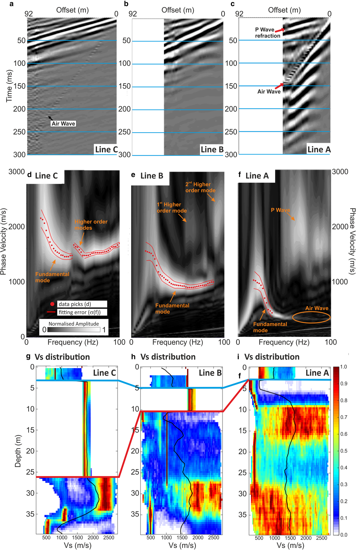
Fig. 8. Mid-line C, B and A CMPCC gathers (a–c), corresponding dispersion images (d–f) and Vs distribution profiles (g–i), with the average of the distribution plotted in black.
The dispersion images shown in Figures 8a–c are similar to the synthetic dispersion images (Figs 6i–l) giving an initial insight into the structure expected at Midtdalsbreen. The dispersion curves, which have a high signal-to-noise ratio, are picked for frequencies between 14 and 100 Hz, implying that the thinnest resolvable layers (L min) are 4.0 m (Line A), 3.8 m (Line B) and 5.7 m (C) and the maximum resolvable depths (L max) are 19.5 m (Line A), 33.5 m (Line B) and 45.7 m (Line C).
The dispersion picks and their estimated uncertainty were supplied to MuLTI, together with the GPR depth constraints. The inversions used the same parameters used in the synthetic study. Posterior Vs distributions are shown in Figures 8g–i, the highest density velocities (coloured red) corresponding to the most likely (modal) solution. The average solution (black line) is the average of all accepted models, displaying a smoothed Vs solution, and its uncertainty is expressed as one-half of the 95% credible interval range at each depth. These uncertainties are typically ±~600 m s−1 for the snow layer, ±~120 m s−1 for the ice layer and ±~1100 m s−1 for the subglacial material. The estimated uncertainty for the mode solution is one-half of the interquartile range at each depth, accounting for the skewed probability densities highlighted in Figures 8g–i. This convention implies smaller uncertainties: ±~250 m s−1 in the snow layer, ±~75 m s−1 in the ice layer and ±320–560 m s−1 in the subglacial material.
The 1-D inversions show low shear wave velocities, 500–1000 ms−1 beneath the constrained snow ice horizon in Line A and the constrained ice-bed horizon in Line B; both are in turn underlain by a high Vs zone, 2000–2500 m s−1. In contrast, high velocities, ~2400 m s−1, occur directly below the thicker ice in Line C. This analysis suggests a spatially variable pattern of subglacial Vs from the front of the glacier to Line C, 150 m up-glacier.
2-D shear wave velocity profiles
MuLTI is used to invert multiple independent 1-D dispersion curves picked from all CMPCC gathers along each seismic line. Offsets are limited either to mitigate body wave contamination or prevent lateral smearing (particularly in line D where the thickness of ice decreases along the line and therefore we do not assume lateral homogeneity of Vs along this line). Dispersion patterns and the implied depth of penetration vary with ice thickness and the likely subglacial Vs, as shown by the depth range of input velocity picks in Figure 9 (leftmost column). These plots represent all 1-D dispersion curves, picked at each CMPCC location along the line, indicate the maximum depth at which inversion results may be considered reliable.
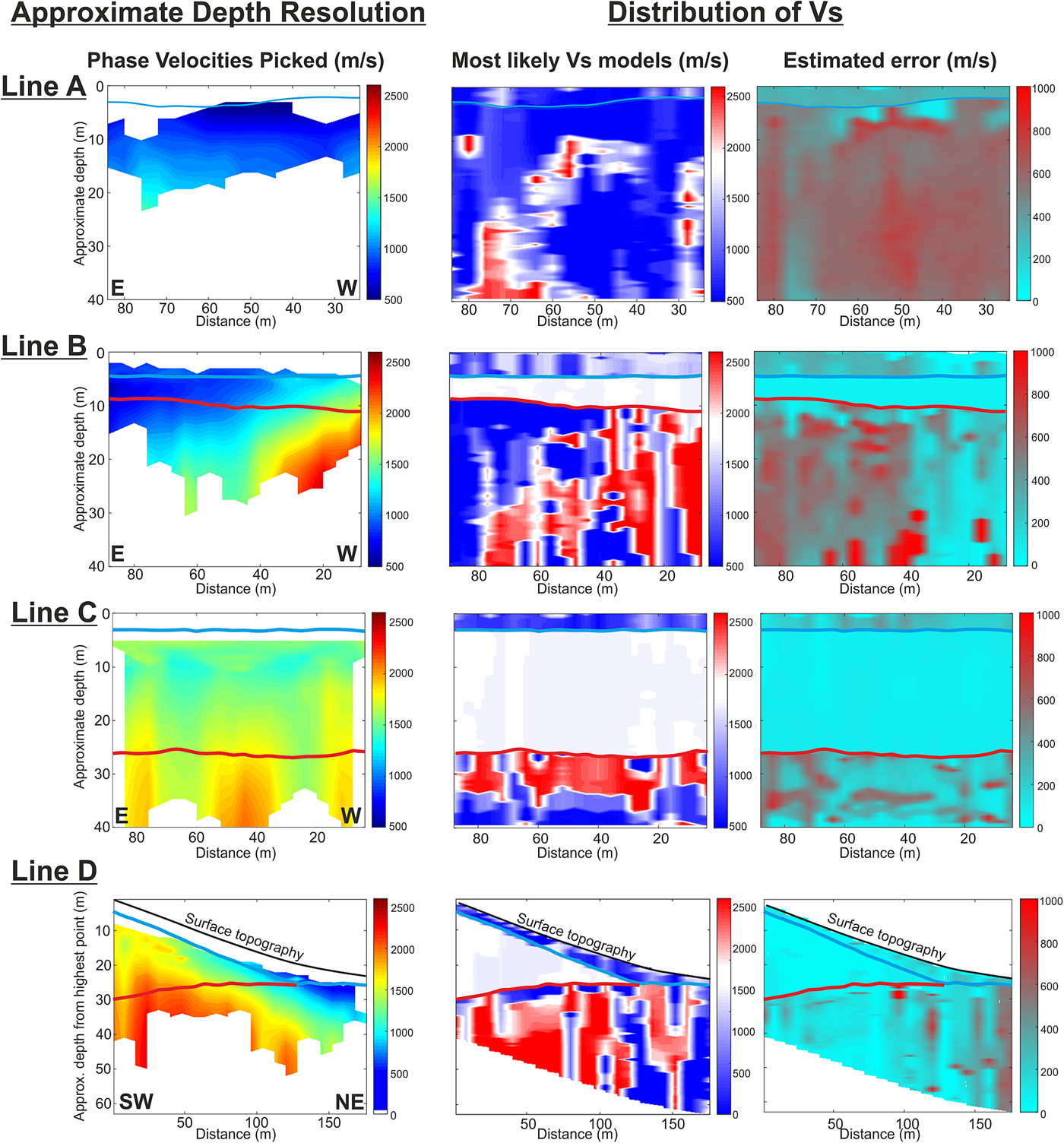
Fig. 9. 2-D inversion outputs for Lines A–D. Left column: approximate 2-D depth resolution, characterised by the range of phase velocity picks. Central column: most likely 2-D Vs profiles output from multiple 1-D MuLTI inversions. Diverging colour scale centred, in white, on Vs of ice (1750–1900 m s−1). Right column: estimated uncertainty (half the interquartile range of the posterior distribution). Snow and ice depth horizons are plotted in blue and red respectively.
Consistent with initial observations in the 1-D analysis, the 2-D Vs profiles (Fig. 9, central column) highlight a wide range of subglacial Vs values, ~500–2500 m s−1. The 2-D profiles highlight spatial variability in Vs for the study region, both along- and cross- glacier profile (the latter evidenced in particular in Line B). The estimated uncertainties for the mode Vs solutions are displayed in Figure 9 (rightmost column). Consistent with the previous analysis, the estimated uncertainties in the average solution are generally very large, especially where input dispersion curve picks are absent (highlighted in Figure S4 in the supplementary material). The corresponding uncertainties in the mode solution are generally smaller, but still increase at depth, to±~1000 m s−1 where Vs constraints are lacking.
INTERPRETATION AND DISCUSSION
Interpretation of Vs profiles
Several studies have inferred subglacial erosion, transport and depositional processes at Midtdalsbreen, based on sedimentological and geomorphological evidence from the glacier foreland (Andersen and Sollid, Reference Andersen and Sollid1971; Etzelmüller and Hagen, Reference Etzelmüller, Hagen, Harris and Murton2005; Reinardy and others, Reference Reinardy, Leighton and Marx2013, Reference Reinardy2019; Willis and others, Reference Willis, Fitzsimmons, Melvold, Andreassen and Giesen2012). However, the type and distribution of subglacial substrate is largely unknown, having not been directly imaged beneath the glacier.
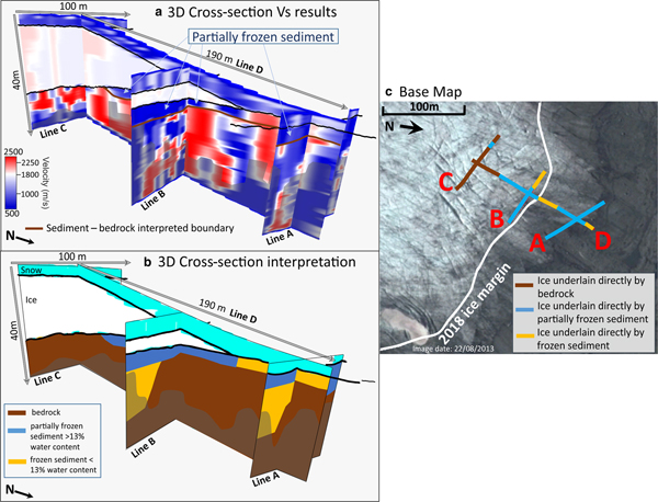
The variability of Vs (500–2500 m s−1) in our MASW records points to a complex subglacial structure, comprising local accumulations of bedrock and softer material, potentially permafrost and/or till, overlying bedrock (Fig. 10). We consider the abrupt lateral variations in the outputs to be noise rather than genuine structure and instead interpret the broader variation in lateral and vertical character as representative velocity structure. The lateral resolution in our imaging varies along each line, given the changing offset range in our CMPCC gathers. In Lines A–C, the limit of lateral resolution is between ±4 and 30 m, and is between ±8 and 40 m in Line D; the poorest resolution is observed in the centre of each line, where the offset range in the CMPCC is greatest. The key structures we interpret in Figure 10 are larger in spatial extent than these limits, hence we consider our lateral resolution to be sufficient.
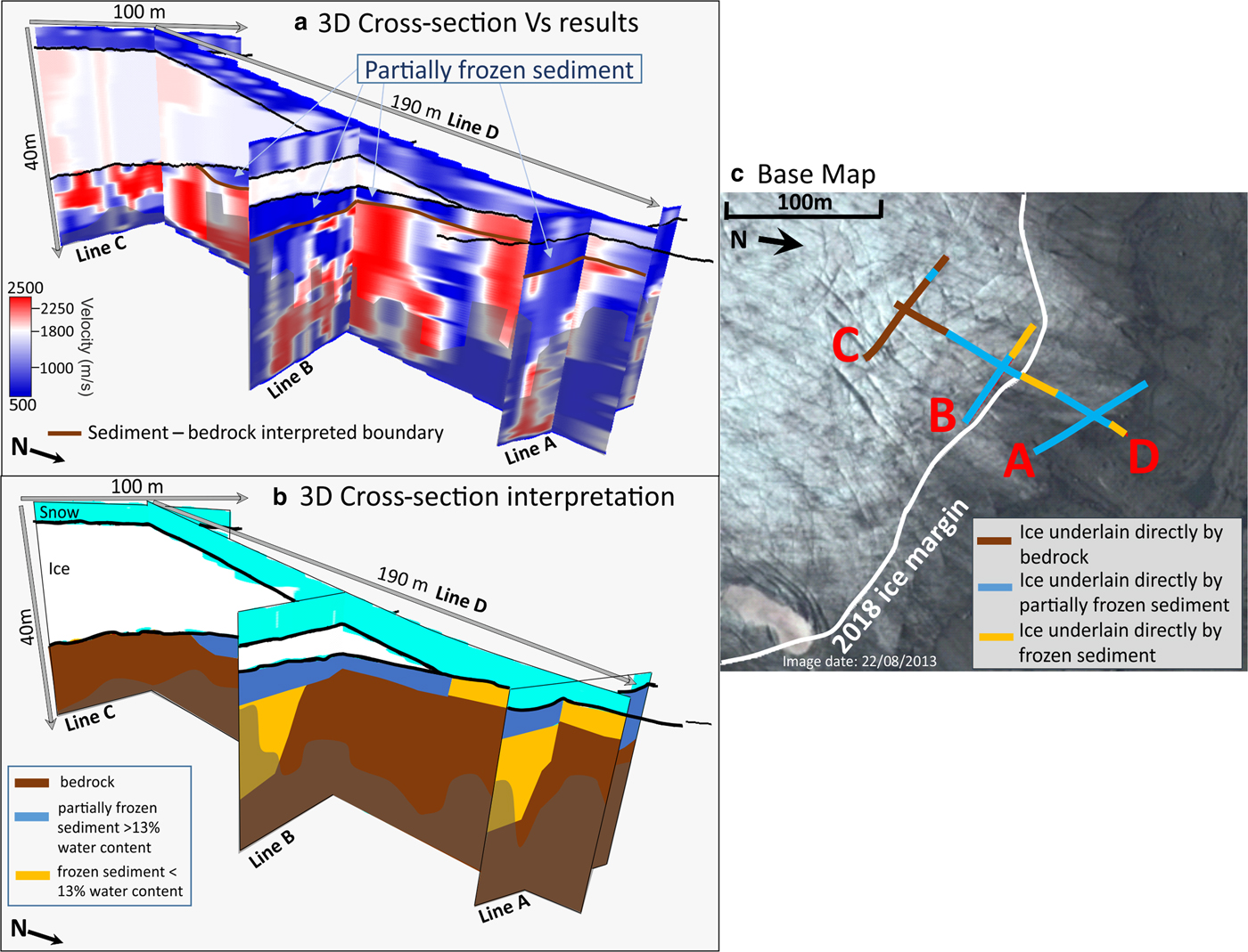
Fig. 10. (a) 3-D cross-section of lines A–D, showing the Vs mode solution and interpreted locations of sediment and bedrock. The black semi-transparent overlay shows where L max is exceeded, hence where results could be unreliable. (b) Schematic 3-D cross-section interpretation of Lines A–D. (c) Base map annotated with line locations and the interpretations from (a).
Our slower velocities (500–1000 m s−1) are interpreted to diagnose various types of partially frozen subglacial sediment, potentially the subglacial continuation of till and silt-rich deposits observed during summer on the glacier foreland. The higher velocities (2000–2500 m s−1) are suggestive of phyllite or granite bedrock, with intermediate values (1000–1700 m s−1) suggestive of frozen zones or weathered bedrock. Kneisel and others (Reference Kneisel, Hauck, Fortier and Moorman2008) suggest that a small increase in the unfrozen water content of sediment, from 10 to 13%, can cause Vs to decrease from 1400 to 600 m s−1, implying Vs is potentially a good means of distinguishing frozen and partially-frozen sediment. Although there is potentially some overlap in our velocity ranges, we use:
• Vs <1000 m s−1 to indicate partly-frozen sediment with water content >13%,
• 1000< Vs <2000 m s−1 to indicate partly-frozen material with water content <13% and
• Vs >2000 m s−1 to indicate bedrock.
Line C suggests that Midtdalsbreen is directly underlain by bedrock 150 m from its terminus, but Line D suggests a transition to a sediment under-burden towards the glacier front. The eastern half of Line B, parts of Line D and all of Line A (on the foreland) are likely underlain by soft (partially frozen) sediment deposits (Fig. 10) with a maximum thickness of 4 m. This thickness approaches our limit of vertical resolution, but uncertainties at the associated depth are low: ±100 m s−1 in Line D and ±280 m s−1 in Lines A–C (Fig. 9). Each inversion also indicates a return to high Vs at depth, consistent with underlying bedrock, although the greater uncertainties at these depths would motivate additional validation (e.g., from a lower-frequency seismic source or an alternate geophysical method such as time domain electromagnetics).
The presence of both bedrock and sediment at the glacier bed suggests that flow both by sliding and substrate deformation is at least possible at Midtdalsbreen, although sub-resolution layers of deforming till may be present where a bedrock substrate is inferred. The implication of zones of basally-frozen and unfrozen regions is consistent with the complex basal thermal regime inferred by Reinardy and others (Reference Reinardy2019), who also suggest that the entrainment and elevation of debris into the glacier requires the substrate to contain both soft and unfrozen material. The presence of thick patches of frozen sediment in the Midtdalsbreen foreland also concurs with permafrost models for this area (Etzelmüller and others, Reference Etzelmüller, Berthling and Sollid2003). In addition to adding constraint to controls on the Midtdalsbreen flow regime, this study may have implications for other valley glaciers and presents a method by which they could be explored.
Discussion and further work
Recurrent problems in Rayleigh wave inversions include poor depth sensitivity, low resolution and ambiguous, nonunique solutions. MuLTI combines a probabilistic approach with external depth constraints, mitigating many of these issues and reducing the size of the solution space. Our probabilistic method allows the uncertainty in any chosen model to be quantified at all depth levels. The addition of depth constraints also improves vertical resolution (Killingbeck and others, Reference Killingbeck, Livermore, Booth and West2018), and further work is required to quantify this improvement.
Nonetheless, the success of MuLTI depends inherently on the quality of the input data and their suitability for the specific target. MASW analyses fundamentally require data to be observed across an array of some minimum length, in order that low frequencies can be faithfully characterised and adequate depth sampling achieved. As such, there is always a loss of lateral resolution for the low-frequency Rayleigh wave related to the array length over which they are observed. This is why we rule out the abrupt lateral variations from our interpretation of Figure 9. We minimise this impact by reducing, where appropriate, the maximum offset in our CMPCC gathers, but the link between lateral resolution and spread-length requires refinement. Any geophysical data are also vulnerable to noise, and we note this for the low frequencies between 50 and 90 m in Line B. If these noisy data were neglected, we would severely restrict the data available for the inversion (Figure S5 in the supplementary material). Instead, we adopt the Bayesian paradigm in which all data are kept but with enhanced error budgets where relevant. Even with their increased uncertainties, these noisy data still provide important depth constraints to the posterior distribution. We note that our data acquisition used 10 Hz geophones, if we corrected our data for the instrument response we may have picked lower frequencies (<10 Hz) which could improve the posterior distribution at depth.
Although this paper focuses exclusively on Rayleigh wave dispersion curves derived from active source seismology, with high-frequency sources and shallow depth penetration, MuLTI can be equivalently applied to dispersion curves from passive sources (e.g., Walter and others, Reference Walter, Chaput and Lüthi2014; Picotti and others, Reference Picotti, Francese, Giorgi, Pettenati and Carcione2017) as the Geopsy forward modelling code, used in MuLTI, has the capability to model dispersion curves with frequencies <1 Hz. Being richer in low frequencies (<20 Hz), these may enable enhanced imaging of structure beneath polar ice sheets (Aster and Winberry, Reference Aster and Winberry2017; Siegert and others, Reference Siegert2018; Yan and others, Reference Yan2018). MuLTI would allow such data to be inverted with depth constraints drawn from radio-echo sounding datasets, thereby highlighting areas of large ice masses with a dynamic sediment underburden, although the algorithm would likely require adaptation to accommodate anisotropy effects.
The MuLTI framework also lends itself well to other geophysical inverse problems, where a theoretical geophysical response for a proposed model can be evaluated and compared probabilistically to observed data. An example of such an inverse problem would be the inclusion of time-domain electromagnetic (TEM) data to the existing approach, to which MuLTI could be readily adapted. Such a combined approach will be the subject of further investigations around the Midtdalsbreen margin, leading to a framework by which aquifer properties beneath large ice masses could be quantified (Hauck and others, Reference Hauck, Bottcher and Maurer2011; Siegert and others, Reference Siegert2018).
CONCLUSIONS
The material properties of the subglacial environment exert a fundamental influence on glacier flow dynamics. These properties can be characterized by considering their shear wave velocity, Vs, obtained by inverting Rayleigh wave dispersion curves. However, conventional dispersion curve inversions lack depth sensitivity and provide solutions that are highly nonunique. Such problems are overcome with the use of our algorithm MuLTI, a transdimensional Bayesian inversion approach, which reduces the ambiguity in the solution space by incorporated independent depth constraints. When trialed for synthetic Vs data representing a small glacier underlain by sediment, inclusion of such constraints results in an order-of-magnitude improvement in the depth-averaged uncertainty in the output model, reducing it for our thickest-ice case from ~1050 m s−1 to ~100 m s−1. While an uncertainty of ~1000 m s−1 may not impede the value of conventional inversions for distinguishing sediment and bedrock substrates, the reduced range would be critical if observations of Vs were to be used to quantify detailed variations in sediment properties. As such, MuLTI is an important advance in the application of Rayleigh wave inversions.
We apply MuLTI to a Rayleigh wave dataset acquired around the terminus of Midtdalsbreen, complementing it with depth-constraints derived from co-located GPR surveys. Although widely underlain by bedrock (Vs ~2500 ± 280 m s−1), our data reveal that a patchy distribution of sediment is present directly beneath the glacier. These sediments are only partly frozen (Vs ~500 m s−1 ± 280 m s−1), and exist in pockets that may be up to 4 m thick; the sediment under-burden extends to ~150 m up-glacier from the terminus. Our interpretation is consistent with recent studies of Midtdalsbreen, which highlight the supply of sediment to the glacier foreland and identify regions of basal sediment around the glacier front.
The seismic data used by MuLTI is supplied in the form of a dispersion curve, hence the algorithm is compatible with Rayleigh wave data obtained from either active- or passive-source surveys. Equally, depth constraints are provided as numerical inputs and can, therefore, be drawn from any external source. MuLTI is therefore applicable for a broad spectrum of seismic data types, as a means of improving the quantitative analysis for a range of contemporary glaciological problems.
SUPPLEMENTARY MATERIAL
The supplementary material for this article can be found at https://doi.org/10.1017/aog.2019.13
ACKNOWLEDGEMENTS
The MuLTI algorithm can be found at: https://github.com/eespr/MuLTI, DOI 10.5281/zenodo.1489959. This project is funded by the UK NERC SPHERES DTP, grant NE/L002574/1. Fieldwork was part-funded by the EVOGLAC project (University of Bergen, University of Oslo) and the research project ‘Snow Accumulation Patterns on Hardangerjøkulen Ice Cap (SNAP)’, itself funded by the European Union's Horizon 2020 project INTERACT, under grant agreement No 730938. Fieldwork was greatly assisted by Emma Pearce and James Killingbeck, and the support and local expertise of Kjell Magne Tangen. Richard Rigby at the University of Leeds is thanked for creating the gpdc mex file. Thomas Bodin is thanked for his advice on MCMC methods and for providing Matlab code. This paper benefited from discussions at the 2017 Glacial Seismology Summer School held at Colorado State University, sponsored by POLENET, SCAR, IGS and IACS. B. Reinardy gratefully acknowledges the support of a Bolin Centre for Climate Research grant.


 Open access