


Introduction
The Sea of okhotsk is regarded as the Southernmost Sea-ice zone in the northern hemisphere except for areas of coastal freezing. it is recognized that the growth and decay of Sea ice is Sensitive to climate change on a global Scale. hence a lot of research has been conducted in terms of the interannual variability of Sea ice in the Sea of okhotsk (e.g. Reference Parkinson, Cavalieri, Gloersen, Zwally and ComisoParkinson and others, 1999). most research has dealt not with volume but with area of Sea ice. this is due to difficulties in monitoring Sea-ice thickness on a large geophysical Scale by either field or Satellite observations. recently, many observations of Sea-ice thickness have been conducted in the Southern Sea of okhotsk. in 1991, the national maritime research institute (nmri) of japan initiated Ship-based video observations of Sea-ice thickness on board the icebreaker Soya of the japan coast guard (Reference Uto, Shimoda, Tamura, Tuhkuri and RiskaUto and others, 1999). Since 1996, the institute of low temperature Science (ilts), hokkaido university, has conducted video observations on board Soya in early to mid-february. based on these Ship-based data, Reference Toyota, Kawamura, Ohshima, Shimoda and Waka-tsuchiToyota and others (2004b) proposed the mechanism of the development of relatively thin ice as a ‘rafting cycle’. the ilts has also conducted Ship-based visual observations. hourly observations of Sea-ice and meteorological conditions were conducted in accordance with the protocol developed by the Scientific committee on antarctic research (scar)/antarctic Sea ice processes and climate (aspect) program (Reference WorbyWorby, 1999). it was found that the deformed ice Such as ridged or hummocked ice comprises up to about 70% of the total Sea-ice volume (toyota, unpublished information). Reference Fukamachi, Mizuta, Ohshima, Melling, Fissel and WakatsuchiFukamachi and others (2003) deployed a moored ice-profiling Sonar near the coast of hokkaido to observe the draft distribution of Sea ice. it was reported that the volumetric fraction of deformed ice is about 70% and 90% of total volume in february and march, respectively. thus, understanding the thickness distribution of deformed ice is a key issue for estimating Sea-ice volume.
The objective of the present Study is to establish a Ship-based method for observing the thickness of deformed ice with reasonable accuracy. it Should be noted that deformed ice is defined as ridged or hummocked ice in this Study. rafted ice is included in the category of level ice. Since 2003, one of the authors has engaged in the core Sampling using a Small basket from Soya (Reference Toyota, Takatsuji, Tateyama, Nakayama, Naoki, Ohshima and IvashintsovToyota and others, 2004a). Since 2004, a Ship-borne electromagnetic inductive (hereafter denoted as Sem) instrument has been used for observing ice + Snow thickness (total thickness). based on the core analysis, the authors developed a model expressing the distribution of direct-current conductivity as a one-dimensional multilayer model. combining this model and theoretical calculation, a new algorithm was developed for transforming the output of Sem instruments to the thickness of both deformed and level ice in the Southern Sea of okhotsk.
Measurement
Sem observations were conducted from 7 to 13 february 2004 and from 12 to 16 february 2005. figure 1 indicates the tracks of Soya during Sem observations in 2004 and 2005. Sea ice normally begins to cover the Southern Sea of okhotsk in late january and reaches a maximum at the end of february. thus these observations were conducted during the ice-growth period. figure 2 Shows the Sites of core Sampling. in 3 years, 26 ice cores were Sampled. among them, 12 cores were Sampled from deformed ice floes. they cover an extensive area below 45.5˚ n. this area is defined as the Southern Sea of okhotsk in this Study.

Fig. 1. Location of SEM observations. Dotted and Solid lines indicate the track of icebreaker Soya during SEM observations in 2004 and 2005, respectively.

Fig. 2. Locations of Sea-ice core Sampling. Empty and filled circles denote the locations of observations in 2003 and 2004, respectively. Empty Squares indicate the locations of observations in 2005.
SEM observations
Sem observation of Sea-ice thickness was initiated by Reference HaasHaas (1998) in the bellingshausen and amundsen Seas, antarctica. a portable, Single-frequency electromagnetic (em) Sensor (EM31/ICE, geonics ltd.) is used to measure the distance (Z E) from the Sensor to the bottom of Sea ice, i.e. Surface of Sea water. figure 3 Shows the Schematic of how the em Sensor measures total thickness. the em Sensor has two coils, a transmitter (tX) and receiver (RX) coil, at each end. a primary em field emitted by TX mostly penetrates Snow and ice and induces an eddy current near the Seawater Surface. this is due to the high contrast in conductivity between resistive Sea ice and conductive Sea water. a Secondary em field caused by this eddy current is detected by RX. the ratio of intensities between the primary (H P) and Secondary em field (H S) is approximately related to the apparent conductivity (σ a) in a uniform half-space:

Fig. 3. Principle of EM observation of total thickness of Sea ice.
Here σ 0 is magnetic permeability of free Space and f and s are frequency (9.8 khz) and coil Spacing (3.66 m), respectively. transformation of σ a into Z E can be obtained either empirically or theoretically. the em instrument can work in either the vertical coplanar (vcp) or the horizontal coplanar (hcp) coil configuration. the authors Selected vcp in terms of its Small footprint Size (Reference Kovacs, Holladay and BergeronKovacs and others, 1995). a laser
Distance Sensor (ld90–3100hs, riegl) detects the distance from the Sensor to the Surface of ice or Snow, Z L. Subtracting Z L from Z E gives total thickness, Z I.
The output of the em instrument was calibrated over ice, nilas and Sea water by the Stepwise changes of Sensor height. the over-sea-water calibration was conducted twice in 2004 and once in 2005. in 2005, over-nilas calibration was conducted once. in the over-ice calibration, drillhole observations on ice were also conducted for determining total thickness within the footprint of the Sensor. the over-ice calibration was conducted twice in 2004 and once in 2005.
Core Sampling
The Sea-ice thickness, Snow depth and ice temperature were observed in Situ. measurement of Salinity and density, thick-and thin-section analysis were conducted at ilts. the ice-core Sampling method is described in detail in Reference Toyota, Takatsuji, Tateyama, Nakayama, Naoki, Ohshima and IvashintsovToyota (2004a).
Data Reduction
Procedure
A one-dimensional, multilayer model is used for transforming σ a into Z E. in general, the conductivity of Sea ice (σ ice) is Small compared to that of Sea water (σ water). for example, Reference HaasHaas (1998) reported that σ ice of the arctic Sea ice was typically 0–30 msm–1 and σ water varies from 2300 to 2900 msm–1. therefore in Some Studies, the influence of σ ice on the transformation from σ a to Z E is neglected. however, deformed ice contains Sea-water- or Slush-filled gaps with high conductivity.
Reference HaasHaas (1998) modeled a high-conductivity layer within highly rotten ice of the Summer antarctic. he treated Such ice as a one-dimensional, four-layer model to derive a transformation formula from σ a into Z E. a high-saline, Slush-and Sea-water-filled gap near the ice Surface was modeled based on the drillhole observations. Reference Tateyama, Uto, Shirasawa, Enomoto, Chung, Izumiyama, Sayed and HongTateyama and others (2004) proposed a multi-rafted model expressing Slush- and Sea-water-filled gaps inside deformed ice in the antarctic. their model was derived by fitting the em responses. in the present Study, the authors analyzed core data to obtain a Semi-empirical model for deriving total thickness of both deformed and level ice from Sem responses. figure 4 Shows the flow chart. the thicknesses of ice block and porosity, which are determined from core data, give the Structure model. the conductivity model is derived from core analysis and conductivity–temperature–depth (ctd) observations. the combination of these two models provides a one-dimensional (1-d), multilayer model expressing the Structure of ice and Sea water. a Semi-empirical model is developed by combining this model, theoretical calculations and Sem responses over Sea water.

Fig. 4. Flow chart for developing model deriving total thickness from SEM response.
Analysis of Sea-ice cores
Twelve deformed ice cores are available in the present analysis. figure 5 Shows one result of the core analysis. σ ice is calculated as follows (Reference HaasHaas, 1998):

Fig. 5. Example of the results of ice-core analysis. Profiles of temperature, Salinity and density are plotted against depth from top Surface of ice. The conductivity of ice is calculated using Equations (2–4) and then plotted against depth from top Surface of ice. Thick-section photo is also Shown. Two horizontal lines in the conductivity panel indicate the estimated gap location.
Here T ice, ρ ice and s ice are temperature, density and Salinity of Sea ice, respectively. the thick-section photo indicates two discontinuities at 0.44 and 1.03 m below the top Surface of ice. figure 5 indicates that these discontinuities accompany high Salinity, conductivity and temperature of ice. thus it is judged that a Sea-water- and/or Slush-filled gap exist at these locations. these criteria are used as a judge of gap locations in deformed ice cores.
Structure modeling
table 1 Shows the Summary of the core analysis of deformed ice. the ice thickness and Snow depth range from 0.92 to 2.55 m, and 0.06 to 0.27 m, respectively. the thickness of the deformed ice is defined by the distance from the top Surface of the ice to the bottom Surface of the bottommost ice block. the thicknesses of the top consolidated layer, keel layer and ice blocks in a keel layer are derived using the criteria described above. porosity is calculated as follows:
Table 1. Summary of core analysis of deformed ice

Due to the difficulty of accurately measuring total core length, the Scatter of porosity data is Significant and one core has negative porosity. thus the maximum, minimum and this negative value are omitted in averaging porosity. the average values are 0.14m for Snow depth, 0.64m for top consolidated-layer thickness, 0.44–0.27m for ice-block thickness in a keel layer and 13% for porosity.
Conductivity modeling
figure 6 Shows the relation between bulk ice conductivity and ice thickness. here bulk means the depth-wise average. bulk ice conductivity has a constant value of 50 msm–1 for ice thicker than or equal to 0.17 m. this is almost identical with values of winter and Spring antarctic first-year ice (35–75 msm–1) reported by Reference Worby, Griffin, Lytle and MassomWorby and others (1999). ctd observations give the Sea-water conductivity near the Sea Surface as 2700 msm–1. it is assumed that the conductivity of a Sea-water- or Slush-filled gap inside deformed ice is the Same as that of Sea water.

Fig. 6. Relation between bulk conductivity of ice and ice thickness.
One-dimensional, multilayer modeling
Combining Structure and conductivity models, a one-dimensional, multilayer model is proposed for representing the internal Structure of Sea ice in the Southern Sea of okhotsk. figure 7 and table 2 Show the Summary of the model. the Snow layer and top consolidated layer are handled as a Single layer. each gap thickness is calculated by multiplying the porosity and the thickness of the ice layer above it. the thickness of the last ice layer is determined by the length to Sea-water Surface.

Fig. 7. One-dimensional multilayer model, expressing Sea water and internal Structure of Sea ice.
Table 2. Thickness and conductivity of each layer

In the present model, up to four layers of ice and gaps are assumed in a keel layer. including the top consolidated layer and Sea water, this model can treat ten layers at maximum. the influence of a highly conductive gap layer on the em response decreases as thickness increases. thus it is thought that the influence of this truncation is Small.
Forward modeling
One-dimensional forward modeling of the em response is performed by the full-solution multilayer analysis of Reference AndersonAnderson (1979). a theoretical calculation program (pcloop, geonics ltd.) can provide transformation of σ a into Z E. firstly, the offset between theoretical calculations and measurements is evaluated as follows. during the voyages in 2004 and 2005, calibration of em responses was conducted over Sea water or nilas within pack ice twice, respectively. in these calibrations, the altitude of instruments was varied in a Stepwise manner. the corresponding em responses were calculated using pcloop by a one-dimensional, one-layer model, representing Sea water. the conductivity of Sea water is Set at 2700 msm–1. figure 8 Shows the comparison of the results between calibrations in 2004 and theoretical calculations. the Solid line denotes the curve fitting of calibration data by exponential function (denoted as ice-free model). although calculations Should be identical with measurements, there exists a certain

Fig. 8. Offset between theoretical calculations and measurements. Two Symbols denote the results by calibration over Sea water in 2004. The Solid line denotes the curve fitting of these data by exponential function. Dashed line indicates the result of Pcloop by using one-dimensional one-layer model representing Sea water. The conductivity of Sea water is 2700 mSm–1.
Amount of offset, probably due to the misalignment of the em instrument. thus modeled responses (σ am) are corrected by equations (7) and (8) in the following analysis:
During voyages in 2004 and 2005, calibration of em responses over deformed ice was conducted twice and once, respectively. figure 9a and b Show the comparison of responses between measurements and calculations in 2004 and 2005, respectively. the total thickness of ice was 2.48 and 2.24 m in 2004 and 2.14 m in 2005. the ice-free model is often used as a transformation formula from σ a to Z E. this is valid in the case of Solid ice Since the bulk conductivity of Sea ice is very Small compared to that of Sea water. however, there is a large offset between calibration data and the ice-free model. this is primarily due to the existence of a highly conductive layer in the deformed ice.

Fig. 9. Validity of the present model: results in (a) 2004 and (b) 2005. Responses using the present model are compared with those observed by calibration over two (a) and one (b) deformed ice floes. Dashed line indicates the ice-free model, given by the least-squares fitting of calibration data over ice-free water. Dates are dd/m/yy.
Notes: Italic indicates the data omitted in averaging. Porosity is defined as the ratio of gap length to total thickness. NA: not applicable.
Modeled responses in 2004 Show reasonable agreement with calibration data. however, modeled responses were underestimated against observations in 2005. this is most likely due to the very high porosity of ice at the calibration Site. the core (no. 0502 in table 1) had porosity of 38%, the highest value in 3 years. however, the modeled response approaches the observed response with an increase of Z E. the Sensor height (Z L) was normally about 4 m during observations. thus 2.14m thick ice gives Z E of 6.14 m, and the difference of responses is Small under Such normal observation conditions.
Inversion
A Series of calculations by the forward modeling are conducted by changing Z L and Z I. the range of Z L and Z I is 1.0–5.5 m and 0.0–5.0 m, respectively. the increment in Z L and Z I is 0.1 m. calculated responses are corrected to σ am_correct using equation (8). a look-up table consists of 46 by 51 σ am_correct. total thickness is obtained by matching measured σ a and Z L with values in this table. if total thickness is <0.78 m, the ice is regarded as level and treated by a two-layer model, i.e. one layer for ice and another for Sea water. the number of layers depends on the total thickness but is truncated to be ten.
Results and Discussions
Validity of the model
The present model has the following morphological parameters of ice: thickness of the top consolidated layer, porosity and thickness of the ice blocks in a keel layer. Reference Toyota, Kawamura, Ohshima, Shimoda and Waka-tsuchiToyota and others (2004b) analyzed the video thickness data collected from 1991 to 2000, except 1995, from late january to late february in the Southern Sea of okhotsk. they reported that the annually averaged ice thickness ranges from 0.19 to 0.55 m. this thickness is regarded as that of the level ice or the top consolidated layer of deformed ice. the modeled thickness of the top consolidated layer (0.64 m) is over the maximum of annually averaged ice thickness. this means the possibility of misinterpreting level ice as deformed ice is quite low, guaranteeing the accuracy of level-ice thickness in the present model.
In general, the porosity of a keel layer of fresh hummocks and ridges is about 20–40% (Reference LeppärantaLeppäranta, 2005). Reference Beketsky, Astafiev and TrusckovBeketsky and others (1996) reported that the porosity of a keel layer and an entire hummock offshore of northern Sakhalin was 20% and 13%, respectively. the present model gives the porosity of the entire deformed ice as 13% and that of a keel layer as 23%. these values are within the range of fresh hummocks and ridges and close to the values by Reference Beketsky, Astafiev and TrusckovBeketsky and others (1996). the thickness of the ice blocks in a keel layer is highly dependent on the mechanism of ridge or hummock formation. more data on the keel-layer Structure need to be collected in order to validate the present model.
Profiles of total thickness
figures 10 and 11 Show the total thickness distributions in 2004 and 2005, respectively. a profile on each day is plotted against distance. the origin of distance is defined at the location where Sem observations Started. Smoothed data in 10 S are plotted at 2 S intervals. during voyages, Simultaneous observations of ice thickness were conducted by using a downward-looking video (Reference Uto, Shimoda, Tamura, Tuhkuri and RiskaUto and others, 1999; Reference Toyota, Kawamura, Ohshima, Shimoda and Waka-tsuchiToyota and others, 2004b) and by drillhole observations.

Fig. 10. Total thickness profiles by SEM during voyages in 2004. The Solid line indicates total thickness by SEM. Circles indicate total thickness by drillhole observations. Dates are yyyy/mm/dd. JST: Japan Standard Time.
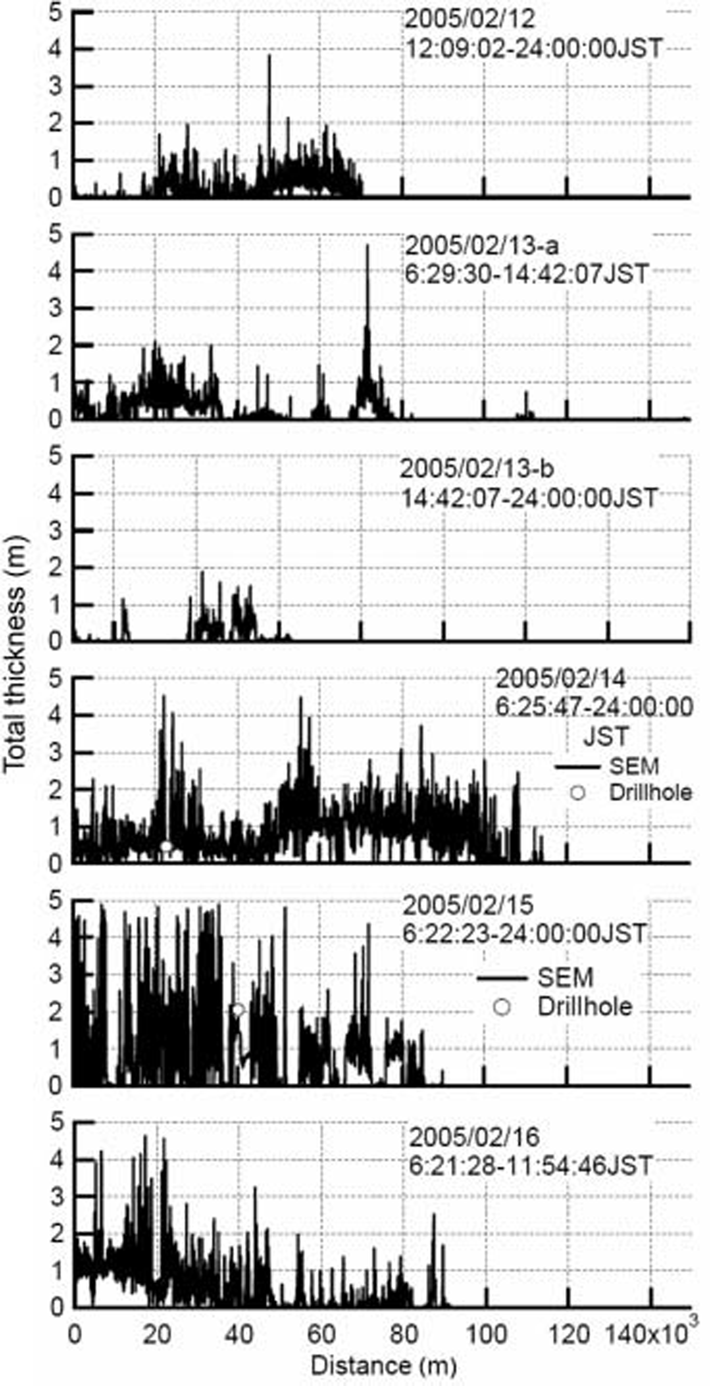
Fig. 11. Same as Figure 10, but for 2005. Profiles on 13 February are divided into two graphs.
figure 12 Shows the comparison of total thickness between Sem and the video method. both datasets on 9 february 2004 are plotted. video observations have no total thickness exceeding 1.5 m, although a general trend between the two datasets is apparent. figure 13 Shows the correlation of total thickness between Sem and video observations on 9 february 2004. here both datasets are averaged in 1 km Segments. it is clearly Shown that video observations underestimate the total thickness against Sem. this is due to the limitation of video observations. in the video method, Sea-ice thickness is measured from floes turned into Side-up positions. in most cases, a loose keel layer of deformed ice is lost during turning. thus the video method mostly observes the thickness of level ice or the top consolidated layer of deformed ice.

Fig. 12. Comparison of total thickness between SEM and video method on 9 February 2004. The Solid line and circles indicate the total thickness by SEM and video observations, respectively.

Fig. 13. Correlation of total thickness between SEM and video observations. on 9 February 2004. Both datasets are averaged in 1 km Segments.
In figures 10 and 11, total thicknesses by drillhole observations are also plotted. both datasets agree fairly well and Sem provides less total thickness than drillhole observations in Some cases. this is probably due to the large footprint of Sem observations. for example, Sem has a footprint with a diameter of about 8m for observing 2 m thick ice at the normal Sensor altitude. furthermore data are time-averaged in 10 S increments. these two factors lead to Smoothing of local peaks in total thickness profiles.
Probability density of total thickness
figure 14 Shows the probability density function (pdf) of total thickness by Sem observations. pdfs are derived from all data in 2004 and 2005. the average total thickness of ice thicker than 0.05 m is 0.61 and 0.75 m in 2004 and 2005, respectively. the maximum total thickness is 4.49 and 4.87 m in 2004 and 2005, respectively.

Fig. 14. Pdf of total thickness by SEM observations in 2004 (empty circles) and 2005 (filled circles): (a) Semi-log plot in the total thickness of 0–5 m; (b) linear plot in the total thickness of 0–2 m. PDF is derived from all data measured in 2004 and 2005. Bin is Set 0.1 m. is almost identical with mean annual maximum thickness of thermally grown ice in the Southern Sea of okhotsk (Reference FukutomiFukutomi, 1952). the most frequent thickness in the range of deformed ice is 0.9–1.1 m, which represents the typical thickness of moderately deformed ice. a larger amount of thick deformed ice leads to a lesser amount of thin level ice in 2005, and vice versa in 2004.
figure 14b indicates that modal thickness in the pdf of 2004 is 0.2–0.3 m, which corresponds to young ice presumably frozen in Situ. two more peaks appear in the ranges 0.5–0.6 and 0.9–1.0 m. the former peak corresponds to the maximum thickness of level ice (Reference Uto, Shimoda, Tamura, Tuhkuri and RiskaUto and others, 1999) in the Southern Sea of okhotsk. the latter peak corresponds to modal thickness in the range of deformed ice. in 2005, there is no peak in the range of young ice. the modal thickness is 0.4–0.5 m, which corresponds to the typical thickness of level ice. the Second peak is found in the range 1.0–1.1 m. this is the modal thickness in the range of deformed ice in 2005.
Both pdfs have a tail which gives a good fit to a negative exponential distribution. interestingly, the Same trend is reported for the distributions of arctic Sea-ice thickness (Reference WadhamsWadhams, 2000). the Slope of a tail expresses the amount of deformed ice. it is clearly observed that the amount of deformed ice was larger in 2005 and that of thin level ice was larger in 2004. thus it is Speculated that in Situ freezing is dominant in 2004 and Southward drift of thick deformed ice is dominant in 2005.
In Summary, there are one or two peaks within the range of level ice. the main peak is in the range 0.4–0.6 m, which
Conclusion
We propose a new model for deriving total thickness by Sem observations in the Southern Sea of okhotsk. Special attention is given to observations of total thickness of deformed ice with better accuracy. based on the results of core analysis, we express the internal Structure of pack ice in the Southern Sea of okhotsk, as a one-dimensional multi-layered Structure. combining this model with theoretical calculation, a new algorithm is developed for deriving total thickness from responses of Sem instruments. the validity of the morphological parameters of ice used in this model is discussed. the thickness of the top consolidated layer is over the maximum of the annually averaged ice thickness observed from 1991 to 2000. this means the possibility of misinterpreting level ice as deformed ice is quite low. comparison with results by video observations Shows an underestimation of total thickness by the video method. this is primarily because of the limitation of total thickness observations by the video method. comparison with drill-hole observations Shows fair agreement. the pdf of total thickness reveals the characteristics of the total thickness distribution. there are two characteristic ranges of thickness. one is 0.4–0.6 m, a modal thickness of level ice. in the range of deformed ice, there is a peak at 0.9–1.1m thickness, which represents the typical thickness of moderately deformed ice observed in the Southern Sea of okhotsk. a larger amount of thick deformed ice leads to a lesser amount of thin level ice in 2005, and vice versa in 2004.
Acknowledgements
We acknowledge the captains and the crew of icebreaker Soya of the japan coast guard for their kind cooperation. we also thank k.i. ohshima of the ilts, m. nakayama of kushiro children’s museum, k. naoki of chiba university, and S. oka and t. takimoto of the nmri for their efforts in conducting field observation.


