


Introduction
Up to the mid-1970s, the topography of Icelandic glaciers was scarcely known. While their extent had been identified (11 000 km2 e.g. Björnsson, Reference Björnsson1979) surface maps were inaccurate by as much as ~100 m of elevation, and the bed topography had only been surveyed at a few dozen places by means of seismic sounding in the 1950s (Eyþórsson, Reference Eyþórsson1952; Holtzscherer, Reference Holtzscherer1954; Rist, Reference Rist1967). Today, however, the topography of the island's major ice caps (Fig. 1) is well known, thanks to depth surveys by radio-echo sounding (RES) and a combination of accurate surface-mapping methods. Following successful depth soundings on temperate glaciers by Watts and his colleagues (Watts and England, Reference Watts and England1975; Watts and Wright, Reference Watts and Wright1981), analogue echo-sounding equipment operating in the frequency band of 2 to 10 MHz was designed and tested in 1976 to 1978 on Vatnajökull (Ferrari and others, Reference Ferrari, Miller and Owen1976; Björnsson and others, Reference Björnsson, Ferrari, Miller and Owen1977; Sverrisson and others, Reference Sverrisson, Jóhannesson and Björnsson1980). Since 1977, this equipment and after 2008 its digital successor has seen use in the continuous thickness profiling of ice caps and valley glaciers in Iceland, Norway and Sweden, as well as in the charting of polythermal glacier beds in Svalbard (Björnsson, Reference Björnsson1981, Reference Björnsson1982, Reference Björnsson1986a, Reference Björnsson1986b, Reference Björnsson1988, Reference Björnsson1996, Reference Björnsson2017; Björnsson and Pálsson, Reference Björnsson and Pálsson2008; Björnsson and others, Reference Björnsson1996, Reference Björnsson, Pálsson and Guðmundsson2000; Magnússon and others, Reference Magnússon, Pálsson, Björnsson and Guðmundsson2012, Reference Magnússon2016). In most years since 1980, the systematic mapping of bedrock topography has extended to all of Iceland's main ice caps: Vatnajökull, Hofsjökull, Mýrdalsjökull, Langjökull and Drangajökull (Fig. 1). At the same time the first glacier surface maps of known accuracy were derived.

Fig. 1. Iceland's major ice caps with their RES line positions. The yellow areas in the insert represent the island's neovolcanic zone. V: Vatnajökull, L: Langjökull, H: Hofsjökull, M: Mýrdalsjökull, D: Drangajökull.
These surveys have uncovered hidden geological structures such as active volcanoes and deep, glacially eroded valleys (Björnsson and Einarsson, Reference Björnsson and Einarsson1990; Gudmundsson and others, Reference Gudmundsson, Pálsson, Björnsson, Högnadóttir, Smellie and Chapman2002; Sigmundsson and others, Reference Sigmundsson2015; Björnsson, Reference Björnsson2017); furthermore, they have proven indispensable for demarcating subglacial lakes and locating jökulhlaup routes (Björnsson, Reference Björnsson1982, Reference Björnsson1988). Not only has the input from RES techniques thus been significant for investigations of glacier–volcano interaction, but the resulting bed and glacier surface maps have benefited studies of meltwater drainage underneath the glaciers. This has provided a basis for delineating entire drainage basins and generating theoretical models of glacier hydrology and dynamics, glacier responses to shifts in climate and mass balance (Flowers and others, Reference Flowers, Björnsson and Pálsson2003, Reference Flowers, Marshall, Björnsson and Clarke2005, Reference Flowers, Björnsson, Geirsdóttir, Miller and Clarke2007, Reference Flowers2008; Marshall and others, Reference Marshall, Björnsson, Flowers and Clarke2005; Aðalgeirsdóttir and others, Reference Aðalgeirsdóttir, Jóhannesson, Björnsson, Pálsson and Sigurðsson2006, Reference Aðalgeirsdóttir2011; Guðmundsson, Reference Guðmundsson2009; Schmidt and others, Reference Schmidt2019). The decade-long surveys have also yielded essential data for glacier inventories and ice volume estimates. Such exploration has also benefited society substantially in terms of informing the planning, design and engineering of roads and bridges, harnessing hydropower, evaluating energy safety and identifying specific natural hazards.
In 1983, the same low frequencies that were present in the pioneering radar technology enabled the discovery of WWII aeroplanes (‘The lost squadron’) submerged by ~80 m of ice in the temperate sheet of south-eastern Greenland (Björnsson, Reference Björnsson2016). Combining the use of lower and higher MHz frequencies has also characterised bed surfaces and the boundaries between cold and warm ice in Svalbard's polythermal glaciers (Björnsson and others, Reference Björnsson1996).
Finally, RES data have enriched scientific acquaintance with englacial characteristics such as tephra layers evidencing volcanic activity (e.g. Brandt and others, Reference Brandt, Björnsson and Gjessing2006).
Development in equipment and accuracy
Ever since the first forays, the instrumentation for RES surveys has included equipment for navigation, altimetry and continuous ice-thickness profiling.
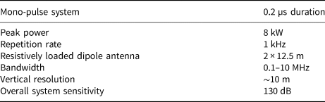
The radio-echo transmitter is a mono-pulse system designed at the Science Institute of the University of Iceland (Sverrisson and others, Reference Sverrisson, Jóhannesson and Björnsson1980; Table 1). Pulses of current, each lasting 0.2 µs and peaking at 8 kW in power, are fed via an avalanche thyristor into a resistively loaded dipole antenna (using two identical antennas) at a repetition rate (frequency) of 1 kHz. While the most commonly used antenna lengths are 2 × 12.5 m, corresponding to a centre frequency of ~3.4 MHz, the antennas have varied from 2 × 5 to 2 × 60 m, i.e. from ~8.5 to ~0.7 MHz. The transmitter and receiver are fastened at the centre of the antennas to sledges which are then towed along the glacier surface by a convenient vehicle (snowmobile, snow-cat or 4WD), typically at speeds of 20–30 km h−1 (Fig. 2). The along-line sampling of the analogue receiver was controlled by a bicycle wheel mounted to the sledge and conveyed trigger pulses that typically resulted in 1 m intervals between individual depth records. From 1977 to 2007, the modulated intensity of the received signal (Z-mode) was displayed on an oscilloscope screen and photographed on a 35-mm camera film (Fig. 2). The sequential pulse signals that were reflected back were logarithmically amplified and stacked (64 to 256 times) in order to increase the signal-to-noise ratio. Clear, continuous signals were returned from depths of up to 950 m. The vertical resolution of the returned signals is around a few to 10 m, depending on the wavelength and signal strength. Starting in 2009, the analogue receiver was replaced by digital receivers using 8 or 12 bit ADCs linked to a laptop computer running the BSI IceRadar survey software (see Mingo and Flowers, Reference Mingo and Flowers2010) that simultaneously collected GPS data as to the time, location and elevation (Fig. 2).
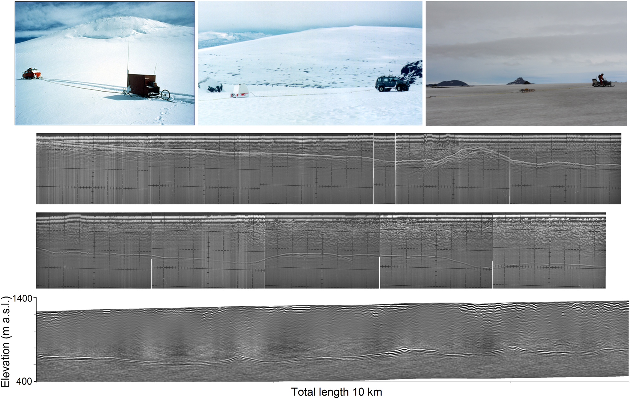
Fig. 2. Top: vehicles towing RES equipment over glacier surfaces in the 1980s, 1990s and 2010s (left to right). Centre: an analogue sounding record of intensity-modulated echoes from a 20 km long RES traverse in the western parts of Vatnajökull. The results on the monitor were preserved by camera on a 35-mm film. Each frame represents 2 µs vertically (~169 m thickness) and 200 m horizontally. Some continuous internal reflections from tephra layers can be seen in this record. Bottom: a 10 km long RES profile from the western area of Vatnajökull. The data has been filtered and migrated, as well as harmonised with surface elevation measurements. The horizontal and vertical scales for this bottom digital record are approximately the same as for the upper two strips which are from analogue records. Internal reflections at shallow depths may indicate properties within the glacier related to englacial hydrology.
Table 1. Characteristics of the echo sounder (Science Institute, University of Iceland)
Where crevasses on the steepest outlet glaciers prevent continuous sounding, single-point measurements are carried out in series, storing the records as amplitude displays (A-scopes). To compute a glacier thickness, the electromagnetic wave velocity has been considered a constant, 169 m µs−1 (which agrees with reference to the Grímsvötn ice cover, where the thickness was measured in a drilled hole). The same constant velocity is applied to the surface firn layer, as its maximum thickness is only about 20 to 30 m. The velocity may vary by a few m µs−1 depending on e.g. water content in the ice.
Navigating the sounding lines
From 1977 to 1979, compass bearings were observed in order to navigate traverses across the ice cap. The distance travelled was derived from the bicycle wheel attached to the echo sounder, and specific positions were marked manually on the sounder film record. The position accuracy of sounding lines from these times is assumed to have been ±200 m. Since 1980, the surveys have been carried out systematically in a regular network of sounding lines. Orthogonal grids were established by geodetic surveying and marked with stakes between 1980 and 1982. This approach allowed for an interval of 500 to 1000 m between the sounding lines, as well as for ±50 m accuracy in horizontal positioning. In addition, the actual geographical position of the grid was fixed at several points by satellite reference (using the Transit satellite navigation system).
From 1982 to 1990, Loran-C (often aided with gyro-compass) was the exclusive means of navigation while traversing the ice caps. During this period, latitudes and longitudes along the sounding lines (in WGS-66 coordinates) were recorded on a magnetic tape at 50 m intervals, resulting in ±50 m accuracy. This expedited the sounding task, saving manpower that had been required for following the sounding lines. Three stations were available for the signals of Loran-C, one each on Snæfellsnes (West Iceland), Jan Mayen and the Faroe Islands. Loran-C was developed for navigation of ships and aircrafts and when used on the land we observed location errors varying from 200 to 500 m, however with a repetition accuracy of ~10 m. This aberration was corrected by comparing Loran readings at known positions outside of the glaciers to a few points within the sounding area that had been pinpointed by standard geodetic survey or satellite navigation (i.e. by GPS). The adjusted positions of these points are considered to have been accurate within ±30 m, making the final position of the sounding lines accurate within ±50 m. For convenience during fieldwork, sounding traverses were often aligned with longitude or latitude.
In 1991, Loran-C was retained to operate in combination with GPS, but as of 1993 GPS orientation became the sole navigation guide. To begin with, this GPS guide improved the accuracy to ±10 m. By 1996, however, GPS accuracy had attained ±1–5 m for such soundings and in 2004 post-processed kinematic land survey achieved ±5 cm. Thanks to navigating advances, field campaigns which till the mid-1990s took a team of five to 12 people from 5 to 6 weeks now require just 1 week for two people.
Aerial photographs and satellite images (Landsat after 1972; Spot, Pleiades), Arctic Dem and Lidar maps have been consulted in order to select optimal sounding lines and avoid dangerous crevasses. In areas of rugged topography, sounding lines have been arranged to obtain angles perpendicular to the steepest expected bedrock slopes, thereby reducing the off-nadir echoes and simplifying wave migration from the actual bottom surface. Figure 1 shows the sounding line scheme from 1978 to 2019. Various photos from the fieldwork appear in Figure 3.
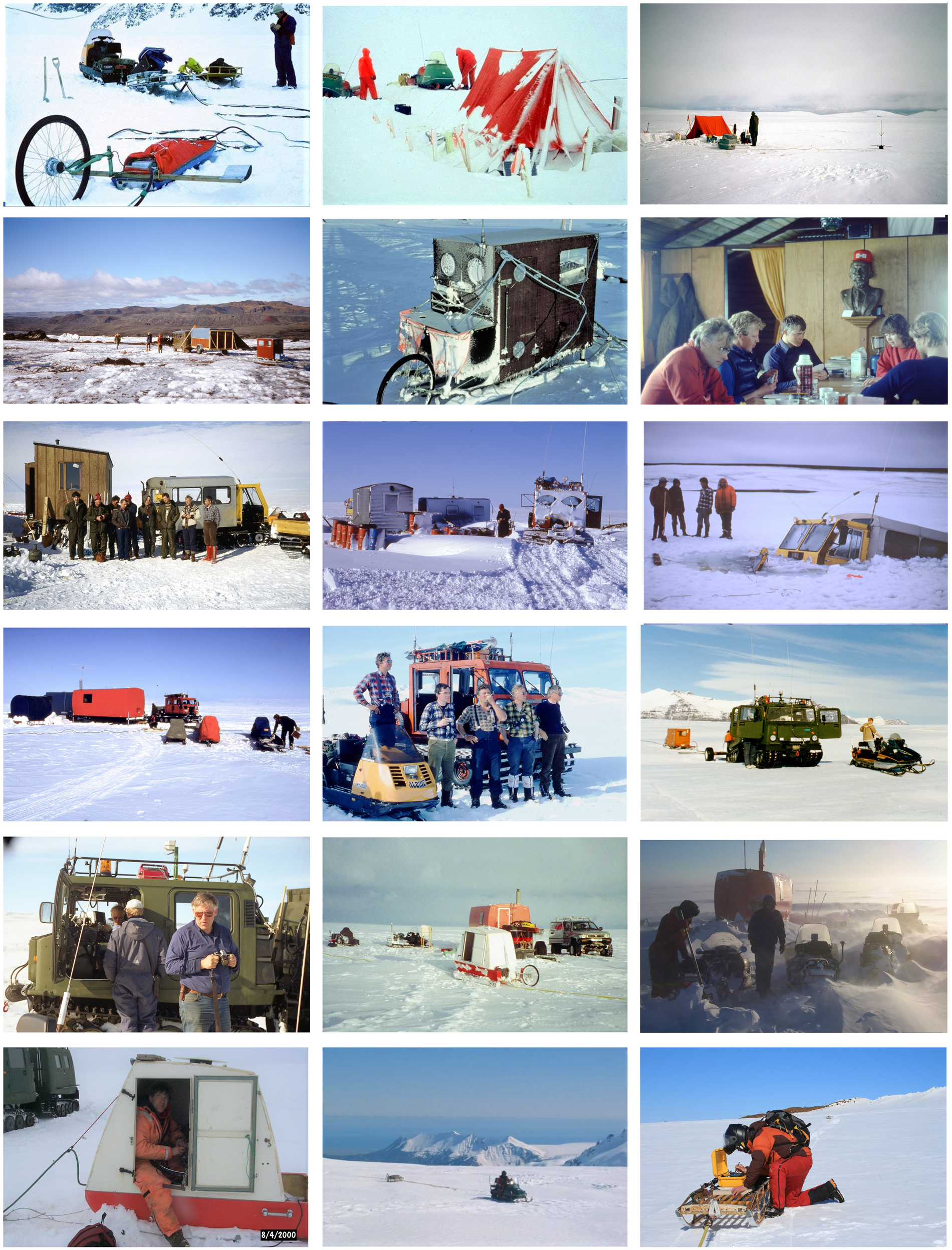
Fig. 3. Photographs from RES fieldwork 1977–2019 (photos: Helgi Björnsson (HB), Marteinn Sverrisson (MS), Hannes H. Haraldsson (HHH), Finnur Pálsson (FP), Sveinbjörn Steinþórsson (SS), Bryndís Brandsdóttir (BB)). Texts for images in this figure, addressed in {row, column}: {1,1} Radar prototype in Grímsvötn, central Vatnajökull, in June 1977 (HB). {1,2 and 1,3} The camp site on Mýrdalsjökull in 1978. The tree like structure is the antenna for the Transit satellite navigation receiver (MS). {2,1} Leaving Vatnajökull in spring 1978, after a successful RES survey in Grímsvötn (MS). {2,2} Survey hut on skis for the RES receiver and the bulky TMS 9900 microcomputer system and positioning equipment in 1980 (HB). {2,3} A break from the RES survey of Tungnaárjökull in the hut of Jökulheimar in April 1980 (MS). {3,1} The survey team at the camp on Eyjabakkajökull outlet, NE-Vatnajökull, in April 1981 (MS). {3,2} Starting the day's work at the camp on Köldukvíslarjökull, NW-Vatnajökull, in April 1982. The expedition suffered 3 weeks of blizzard at the beginning, unable to work, followed by 3 weeks of successful survey (HHH). {3,3} On the way home after 6 weeks of RES on Köldukvíslarjökull, NV-Vatnajökull, in 1982. The ice on a lake gave in (HHH). {4,1} Starting the day's RES work early in the morning at the camp on Hofsjökull in April 1983 (HHH). {4,2} Admiring the views on Hofsjökull in April 1983 (HHH). {4,3 and 5,1} RES on Breiðamerkurjökull, S-Vatnajökull, just above the calving front of Jökulsárlón in April 1991. Antenna rods for the LORAN-C navigation equipment visible on the receiver hut and both vehicles, also the GPS egg-shaped antenna on snow-track roof (FP). {5,2} The camp on Skeiðarárjökull, S-Vatnajökull in 1994, the first use of a new receiver hut (FP). {5,3} The camp on Tungnaárjökull, W-Vatnajökull, after a blizzard in April 2000. Digging out the snowmobiles (FP). {6,1} Fixing a broken wire on Tungnaárjökull in April 2000 (HHH). {6,2} GPS and laptop computers allowed compaction of the receiving equipment into one box, fit on a Nansen type sled. The RES survey on Fláajökull, SE-Vatnajökull, in May 2003 (SS). {6,3} Starting a survey with the Blue System Integration RES receiver on Vatnajökull in June 2019 (FP).
Mapping ice surface elevations
From 1977 to 1994, altitudes at the ice surface were derived through precision barometric altimetry. Air pressure was logged continuously where the echo sounder was dragged over the ice surface, while air pressure readings throughout the same time were recorded at base camps where the elevation was known (Björnsson, Reference Björnsson1988). In addition, corrections were made for the effects of air temperature variations. All elevations were referenced to points of known altitude on neighbouring mountain peaks and at land survey triangulation sites. Occasional surveys on the glacier provided optically levelled profiles for height references, with an elevation accuracy of close to 1 m. Until 1981, the barometer was read manually at 100 to 300 m intervals along the sounding lines, marking the reading positions on the film record of the echo sounder. Beginning in 1982, a barometric altimeter was employed which entered recordings automatically on a magnetic tape at 50 m intervals along the sounding lines (together with the Loran-C positions). The absolute accuracy in elevation figures was better than ±10 m on the sounding lines, and the relative elevations were accurate to the order of ±5 m. The difference in surface elevations at crossing points was less than 5 to 10 m at nearly every point. The uncertainties were caused by altimeter calibration errors, locally varying air pressure and discrepancies in the crossing-point locations. Between 1995 and 2004, elevations were recorded based on differential GPS, with an accuracy of 1 to 2 m, and as of 2005 through continuous kinematic GPS profiling, with accuracy in the decimetre range (e.g. Trimble Engineering and Construction Group, 2009). By then the uncertainty was mostly due to the erratic motion of the GPS antennas relative to the surface.
Data reduction
In the analogue system of continuous photographic sounding records, the bedrock echo was digitised at points separated by an over-snow distance of some 25 to 50 m. Since 2009, the RES records are digital. Two-dimensional migration is performed for the echo profiles, assuming the echoes arise from within the vertically oriented plane perpendicular to the antennas. The ice thickness along the sounding lines represents a smoothed profile that does not represent the highest and lowest points in the landscape. Instead, the echo sounder perceives a strip along the bed which is typically ~100 to 200 m wide. The width, d, can be defined by the first Fresnel zone as

We can identify the echo's arrival time to the nearest quarter of a pulse length, where r is the shortest distance down to the bed and λ is the pulse length. In our soundings λ is about 30 m and thus for r = 100 m, d = 60 m, while for r = 600 m, d = 200 m. The result is the final geographical position of the points of reduced ice thickness on the sounding line. The accuracy for ice thickness along the sounding lines is assumed to be ± 15 m. About 80% of all crossing points differed with regard to ice thickness by less than 20 m.
The bedrock elevation is obtained via the difference between the ice thickness and the altitude of the ice surface. Figured this way, the average absolute bedrock uncertainty is estimated to be ± 30 m.
Elevation maps of bedrock and ice surface topography have been compiled by interpolating data from our widely spaced survey lines (typically with intervals of 1000 m) and connecting to the existing geodetic maps of areas surrounding the ice caps. Firstly, preliminary bedrock digital elevation model (DEM) is calculated typically using the Kriging interpolation method. Subsequently, the contour map is redrawn by hand in order to eliminate obvious error due to sparse data sampling, such as caused by the tendency of contours to appear perpendicular to the sounding lines on account of the much higher data density directly on the routes than between them. Furthermore, based on our knowledge of the landscape, we draw realistic ridges and valleys to replace multiple blobs, highs, dips and voids. Finally, these contours are digitised in order to derive a new DEM, in some cases through an iterative process. This method has been applied to both bedrock and ice-surface DEMs and obviously includes human interpretations of the data rather than purely arithmetic data reductions. Whereas the first DEMs were 200 × 200 m regular grids, advanced computing power and data capacity have permitted calculations with higher resolutions. Recently, defined areas have been surveyed with such short distances between sounding lines (~20 m) as to allow for 3D migration (Magnússon, personal communication). This campaign is resulting in high-resolution (~0.5 to 10 m) glacier surface DEMs based on several remote sensing methods, with GPS surface profiles also aiding local corrections and adjustments to RES survey data.
Topographic details from radio-echo surveys
Table 2 summarises the RESs carried out on Icelandic ice caps, and the locations of the sounding lines appear at a glance in Figure 1. The glacier surface maps compiled from the information gathered became the first elevation maps where errors could be quantified and were suitably small. Comparison with previous maps brings out striking dissimilarities at elevations above 1000 m, in which instances the older maps often underestimated the altitude by 50 to l00 m. Concomitantly, the ice-dome shapes had never been shown correctly. The novel mapping information has since been used to locate the ice divides around outlet glaciers, to determine ice flow lines and to depict exactly the ice cauldrons at glacier surfaces that are created by subglacial geothermal melting and remain largely concealed as water-filled cupolas that may abruptly contribute to a jökulhlaup (see e.g. Björnsson, Reference Björnsson1988).
Table 2. Summary of RES conclusions on Icelandic glaciers
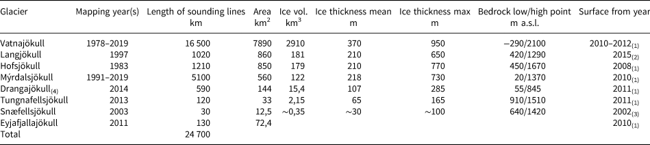
These results present the status in 2019.
(1) Jóhannesson and others (Reference Jóhannesson2012); (2) Porter and others (Reference Porter2018); (3) Jóhannesson and others (Reference Jóhannesson, Björnsson, Pálsson, Sigurðsson and Þorsteinsson2011); (4) Magnússon and others (Reference Magnússon2016); (5) Gunnlaugsson (Reference Gunnlaugsson2016).
Bed maps based on RESs have added significantly to the understanding of land geology and geography beneath Iceland's main ice caps (Fig. 4). Such maps show topographical features and landscape deviations on a regional scale (in the order of kilometres). Due to the wide spacing between sounding lines (typically 500 to 1000 m) the most of the topographic maps do not yet fully reproduce features smaller than 1 to 2 km across. Directly along the sounding lines, however, much more minute details have been brought forth.
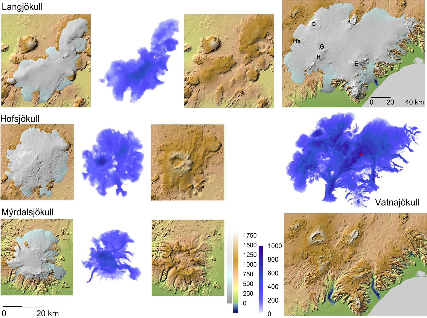
Fig. 4. Maps of the glacier surface, thickness and bed, as produced through RES. (a) Langjökull, (b) Hofsjökull, (c) Mýrdalsjökull, (d) Vatnajökull (G: Grímsvötn, B: Bárðarbunga, K: Kverkfjöll, E: Esjufjöll, H: Hábunga, Ha: Hamarinn). A red star on the map of Vatnajökull's ice thickness indicates the site of the maximum ice thickness.
In general, the island's ice caps originally formed on mountain clusters until completely covering them, leaving only a few nunataks protruding. The thickest ice, 600 to 900 m deep, is found above deep valleys in the ice cap interiors, as well as over huge ice-filled calderas which, inside the highest rims, measure up to 10 km in diameter and 60 to 100 km2 in area. The maximum ice depth that has been discovered is about 950 m, in the central regions of Vatnajökull (Fig. 4). RES surveys reveal that the four largest ice caps, currently covering an area of roughly 10 000 km2, contain ~3400 km3 of temperate ice, equivalent to ~25 years of Iceland's average precipitation. Typically, only 10 to 20% of an ice cap's bed lies above today's glaciation limit of 1100 to 1200 m in altitude. Should the ice caps disappear, they would therefore be unable to reconstitute themselves in the climate characterising the first decades of the 21st century.
A dozen outlet glaciers have been shown to be eroding trenches below sea level, some extending into deeper troughs that were scoured tens of kilometres into the offshore continental shelf by earlier ice-age glaciers. During recent glacier retreat, marginal lakes have gradually been replacing the ice tongues in over deepened depressions. Breiðamerkurjökull (Björnsson, Reference Björnsson1996) and Skeiðarárjökull, two of Vatnajökull's most active outlet glaciers, have excavated trenches up to 200–300 m below sea-level as far as 20 km inland.
Geological structures
Bedrock mapping under the major ice caps has revealed hidden geological structures in Iceland's active volcanic zone (Figs 1 and 4), clarifying how the subglacial landscape is dominated by several large central volcanoes which each feed extensive volcanic system. Radiating outwards, subglacial fissure eruptions have built up linear northeast-southwest trending hyaloclastite ridges and crater rows (Björnsson, Reference Björnsson1988; Björnsson and Einarsson, Reference Björnsson and Einarsson1990). In the west, Langjökull has formed over a row of separate shield volcanoes (which are signals of previously ice-free conditions), as well as over tuyas (where mountain summits standing above the ice cover were covered by lava). Furthermore, Langjökull has built itself up over hyaloclastite ridges and, in the northernmost reaches, over a huge mountain composite piled up by subglacial eruptions. Hofsjökull and Mýrdalsjökull are each borne up by a single colossal central volcano containing huge calderas. The country's largest volcano lies beneath Hofsjökull and was the midpoint of volcanic activity in today's Central Highlands during the Quaternary Period. Farther southeast, Mýrdalsjökull covers the Katla caldera (Björnsson and others, Reference Björnsson, Pálsson and Guðmundsson2000). Underneath Vatnajökull, five central volcano complexes have been discerned: Hamarinn, Bárðarbunga, Háabunga, Grímsvötn, Kverkfjöll and Esjufjöll (Fig. 4). The centre of Iceland's North Atlantic hot spot is located under the northwestern corner of Vatnajökull (Bjarnason, Reference Bjarnason2008). East of the neo-volcanic zone, Vatnajökull's subglacial landscape has undergone substantial glacial erosion, the most prominent features of which are valleys bordered by mountains at the glacier margins.
Several of the depressions found in glacier beds will fill with lakes if the ice over them vanishes. Some of these depressions are extensions of existing marginal (proglacial) lakes that will continue to expand rapidly in the warming climate, like those appearing at the southern margin of Vatnajökull. Modifications in drainage from these marginal lakes are of practical importance in district planning, due to significant areas that may soon become glacier-free.
Watersheds and jökulhlaup routes
Iceland's major ice caps drain into numerous rivers. Static models of the basal watersheds have been constructed. Assuming the basal water pressure to equal p w = k d ρ ig, we can calculate the hydraulic potential at the glacier bed as
where d is the local thickness of the glacier, z is the elevation at its bed, ρ w and ρ i are the densities of water and ice, g is the gravitational acceleration and k is a constant, ⩽1. The drainage routes travelled by jökulhlaups from known sources into particular rivers suggest that the basal water pressure approaches overburden, i.e. k ~ 1 (Björnsson, Reference Björnsson1988). Figure 5 shows a static model of the basal drainage basins under Vatnajökull. Such models of static potential have proven their practicality for estimating runoff to hydropower stations and for the site selection and design of roads and bridges. The surface and bed elevation have provided important constraints in studies of jökulhlaup dynamics and basal sliding along jökulhlaup routes (i.e. Magnússon and others, Reference Magnússon, Rott, Björnsson and Pálsson2007, Reference Magnússon, Björnsson, Rott and Pálsson2010; Einarsson and others, Reference Einarsson2016). The models also enable civil authorities to evaluate the hazards along jökulhlaup routes in cases of subglacial volcanic eruptions or massive drainage from subglacial lakes. When seismic activity has pinpointed the location of a subglacial eruption, the watershed maps have helped to predict the course of a potential jökulhlaup and to warn of likely danger.
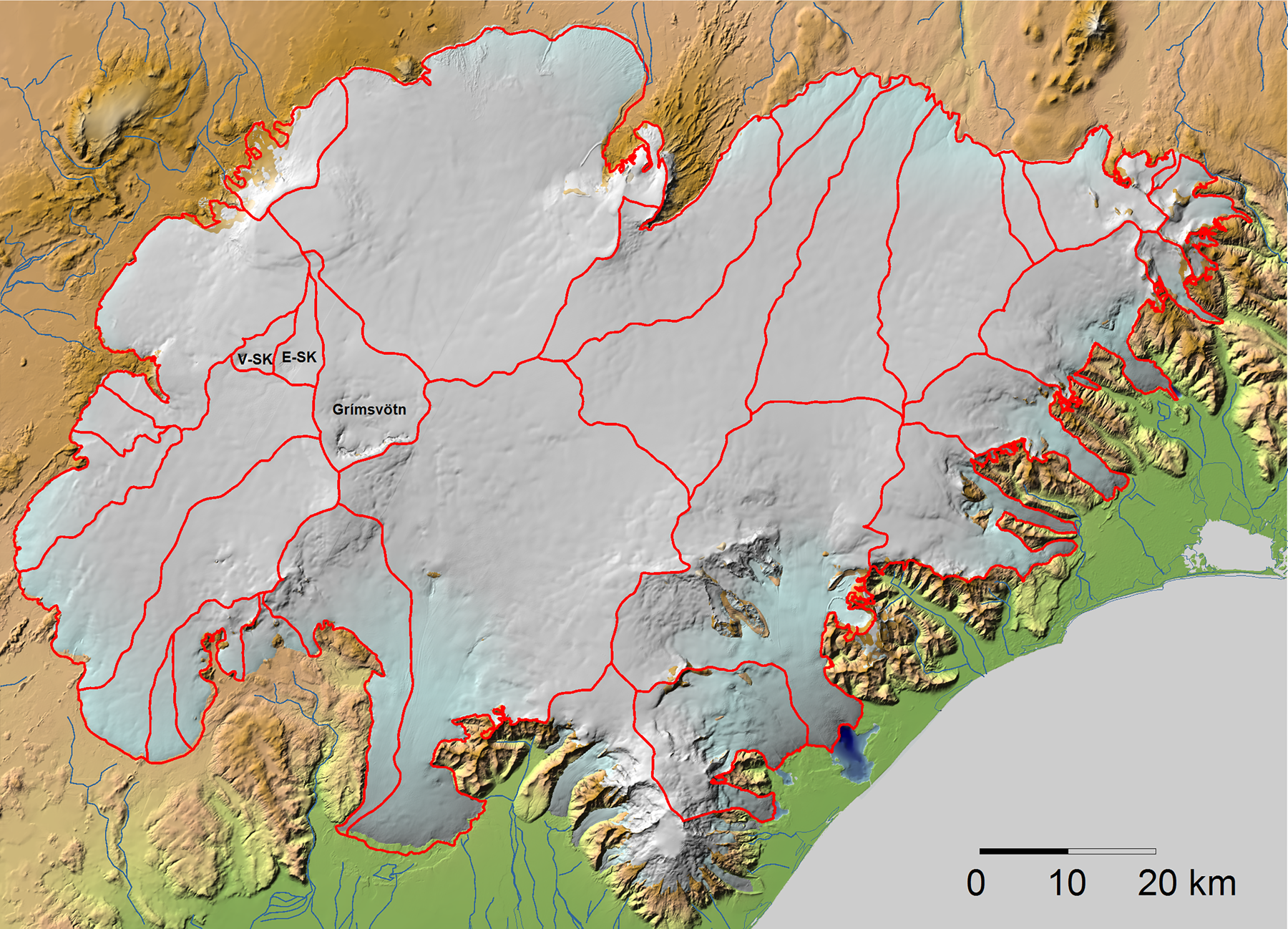
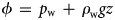
Fig. 5. Watersheds of the main drainage basins of Vatnajökull, as deduced from a static potential model. Subglacial lakes are indicated at Grímsvötn and the two Skaftá cauldrons, E-Sk and V-Sk.
The positions of subglacial lakes can be recognised through depressions in the glacier surface which result from substantial geothermal melting at the glacier bed. The liquid water that becomes trapped and accumulates in such lakes stems from several sources: water percolating downwards from the glacier surface, meltwater produced at the glacier bed and hydrothermal fluid circulating upwards into the lake.
Subglacial lakes
The extent and shape of subglacial lakes have also been circumscribed by means of RES. The ice–water surface of the liquid body can be identified in RES recordings as a smooth interface of strong, constant echo reflections (Fig. 6). Close to the grounding line, where the ice begins to float over the subglacial lake, the radar sees some distance down into pure lake water. Although RES does not penetrate the geothermal fluid in subglacial lakes, their bed topography has been mapped by seismic soundings and in some cases by RES after water has drained out of the lake in a jökulhlaup (Björnsson, Reference Björnsson1988; Gudmundsson, Reference Guðmundsson1989). Repeated RES passes have enabled the estimation of changes in the ice thickness above basal lakes, and thereby the estimation of variations in their water volume (Björnsson, Reference Björnsson1988; Reynolds and others, Reference Reynolds, Gudmundsson, Högnadóttir and Pálsson2018).
Fig. 6. Upper frame: RES profile showing the interface between ice and the subglacial lake named Grímsvötn. The survey was performed at the beginning of a jökulhlaup from Grímsvötn in June 2018, during which the ~300 m thick ice shelf dropped by ~25 m. The lower frame shows the profile route, together with slope shading obtained from an Arctic DEM of 24 August 2017.
Typically, electromagnetic waves rebound stronger from an ice–water interface than from an adjacent wet ice-bedrock face. Everywhere the basal temperature in Icelandic glaciers is at the pressure melting point; the winter cold wave in the glacier surface is eliminated every summer (both in the accumulation zone and the ablation zone). The geothermally-derived basal melt under Vatnajökull has been estimated to account for ~5% of the annual glacial discharge (Flowers and others, Reference Flowers, Björnsson and Pálsson2003).
Internal reflections
Even though our echo sounders were not designed especially for detailed studies of englacial characteristics, considerable internal reflections have been observed that scatter significant energy and therefore diminish the bedrock returns (Fig. 2). Some of the internal reflections are not simply random clutter and may indicate properties within the glacier related to crevasses and englacial hydrology. In the accumulation zones of Icelandic glaciers, we often observe a clear reflection from a water level at 20–30 m depth at which point snow has transformed to impermeable glacial ice. Both ice core and hot water drilling confirm the occurrence of the water table and sporadic water-filled voids (of metre-scale) in the near surface depths of the glaciers. Potential for further study of this englacial hydrology remains to be explored in our data but has been studied successfully by Murray and others (Reference Murray, Stuart, Fry, Gamble and Crabtree2000), Gusmeroil and others (Reference Gusmeroli, Murray, Barrett, Clark and Booth2008) and Matsuoka and others (Reference Matsuoka, Thorsteinsson, Björnsson and Waddington2007).
An entirely different example comprises RES surveys that have yielded information about volcanically produced tephra layers in the ice caps. Across long distances in the interior of Vatnajökull and Mýrdalsjökull, continuous internal reflections can be traced as far down as 400 to 500 m (Fig. 2). Where the same reflecting ash layers outcrop in ablation zones, they can be dated by tephrochronology. Such layers contain basaltic particles mixed with ice (whereby the sand composes up to 50% of the volume and the layer may be tens of centimetres thick as identified in ice cores (Steinthórsson, Reference Steinthórsson1977). All the soluble chemicals in the tephra have been washed out of such interior layers by meltwater. However, layers up to 20 cm thick and as low as 10% tephra by volume may be detected down to 500 m by our sounding instruments, which have a sensitivity of 130 dB, assuming 5 dB/100 m attenuation in pure ice.
This can theoretically be supported as follows. A reflection coefficient of

is expected when a wave of length λ hits an internal layer of thickness h where the dielectric coefficient increases by Δɛ (de Robin and others, Reference de Robin, Evans and Bailey1969; Harrison, Reference Harrison1970). In a layer containing a mixture of ash and ice, whereby the ash has a dielectric coefficient of ɛ 1 and the ice of ɛ 2, we may expect

where m is the volume ratio of ash (0 < m < 1) (Stratton, Reference Stratton1941). If we assume ɛ 1 = 5 for ash in a layer with 10% ash by volume and assume ɛ 2 = 3.17 for the ice, we may expect a wavelength of λ = 34 m to be reflected with a coefficient of R = 1.96 × 10⁻⁸ or −77 dB.
Internal reflections may be caused by layers of bubble-free ice (as observed continuously throughout 1 to 2 m lengths of a Bárðarbunga ice core; Björnsson, unpublished). For a layer 1 m thick, we may expect R = 3.55 × 10⁻⁸ or −74 dB, assuming a jump in density of Δρ = 1.2 kg m−3 and (Δɛ/ɛ) = 1.7 × 10⁻³Δρ, where Δρ is in kg m−3. However, we do not expect such continuous bubble-free layers to exist across major expanses of the glacier.
Much scattering of radio waves is observed in the vicinity of the Gjálp and Grímsvötn area where eruptions are frequent, and layers of tephra have been buried with snow. From direct field observation we know that crevasses formed during the 1996 Gjálp eruption were partly filled with volcanic ash, and heaps of tephra also collected on the glacier surface. After the Grímsvötn eruption in May 2011 a few 100 km2 of Vatnajökull were covered with volcanic ash, in some areas thick enough (>1–10 cm) to hinder surface ablation. But in other areas with thinner tephra melt was enhanced, producing abundant furrows on the glacier surface, a few metres wide and 1–5 m deep, typically, up to tens of metres long, located between elongated ridges, topped with volcanic ash.
Tephra layer evidence of subglacial eruptions
Subglacial volcanic eruption sites have been revealed in RES through higher rates of attenuation and internal scattering. The most outstanding instance is located 5 km north of Grímsvötn, where the basal return echo was so weak that the bed 500 to 700 m below could only be observed with a 60 to 100 m long receiving antenna (1 MHz). This was in an area where a subglacial fissure eruption had taken place in 1938. Every visible sign had been erased in only 15 years, leaving a glacier surface that was completely flat, with no indications of any locally pronounced basal melting. In 1996 a second known eruption took place in the same vicinity, producing a chaotic mixture of ice blocks of metre scale and thick ash layers.
At other sites, single internal ash layers dip down in a circular funnel structure that signifies high basal melting, either due to a subglacial volcanic eruption or continuous, significant geothermal melting (Fig. 7). Tephra layers at eruption sites may either have been deposited onto a flat glacier surface before basal melting took place, or in depressions that were present on the glacier surface and later filled over with accumulating snow and flowing ice.
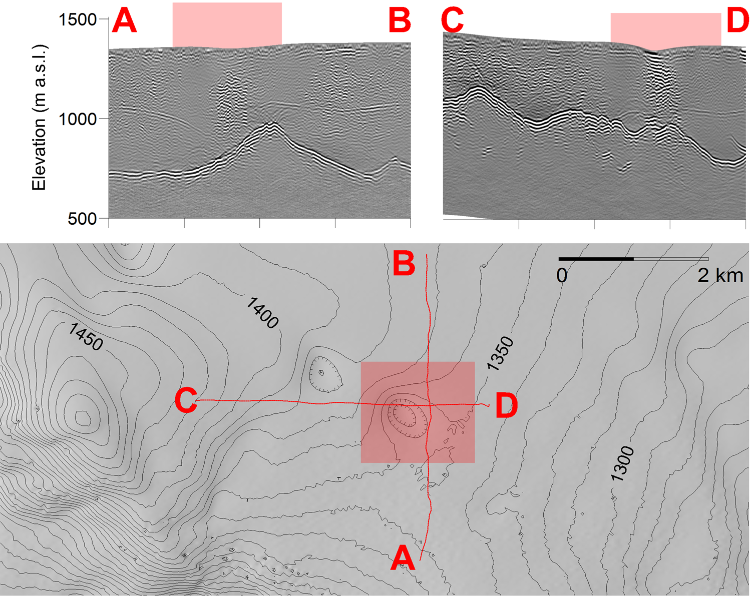
Fig. 7. A funnel-shaped arrangement of tephra layers above a known spot of high geothermal melting.
As the dyke for flowing magma was formed at the onset of the Holuhraun eruption in 2014–2015, three cauldrons formed in the surface of Dyngjujökull above the dyke (Sigmundsson and others, Reference Sigmundsson2015). The cauldron areas were RES surveyed to check for possible water bodies or erupted material at the glacier bed. Indication of tephra intrusion into ice is interpreted from the RES of the northern most of these cauldrons (Reynolds and others, Reference Reynolds, Gudmundsson, Högnadóttir, Magnússon and Pálsson2017).
Concluding remarks
The development of RES in the mid-1970s resulted in the construction of a low frequency analogue echo system (and after 2009 its digital successor) which has been used to explore all the main temperate ice caps in Iceland. The surveys have provided basic data on Icelandic glaciers, of both practical and theoretical importance. They uncovered previously unexplored landforms and geological structures in Iceland's active volcanic zone, yielded data for glacier inventories and ice volume estimates, demarcated subglacial lakes and made possible generation of theoretical models of glacier hydrology and dynamics, e.g. glacier responses to shifts in climate and mass balance. Water catchments of glacier-rivers have been broadly delineated and jökulhlaup routes located. The subglacial topography enables predictions about the growth of proglacial lakes as glaciers retreat during global warming. When eruptions occur under glaciers, hazard warnings on where the meltwater will flow have also been made more dependable. Such exploration has benefited society substantially in terms of informing the planning, design and engineering of roads and bridges, harnessing hydropower, evaluating energy safety and identifying specific natural hazards. The echo-sounding technique continues to prove its potential for investigating the internal properties of glaciers, such as their englacial hydrology, quantification of water volumes beneath cauldrons in areas of high geothermal output and buried tephra layers that shed light on volcanic activity, geothermal activity and past mass balance history.
Acknowledgements
The work was supported by The National Power Company of Iceland, The Road and Coastal Administration of Iceland, The Parliament Financial Committee and the Research Fund of Eggert V. Briem. Special thanks to our colleague Eyjólfur Magnússon who processed the digital RES and for fruitful discussion on the paper content. We are grateful to Philip Vogler for improving the English text of the manuscript.


 Open access