


1. Introduction
Flat-top glaciers are widespread in central Asia. They contain important paleoclimatic information that can be extracted from ice cores. Therefore, features of flow of such glaciers have to be studied for proper interpretation of the information preserved therein. Moreover, these glaciers are important sources of fresh water in the central Asian region, so prediction of the evolution of such glaciers is of special interest.
The Gregoriev ice cap is representative of flat-top glaciers located on the south slope of Terskey Ala Tau, Tien Shan (Fig. 1). Its average ice thickness is 100–110m, while its maximum length and width are 3.7 and 3 km, respectively. It is a cold glacier without bottom sliding. Taking into account the measured data and using a flow model, which takes into account the transverse change of glacier width, we derive an evolution of the glacier shape, velocities and stresses in the ice, and predict the thermodynamic state from 2000 for the next 50 years.

Fig. 1. Map (σ) and longitudinal profiles (b) of the Gregoriev ice cap.
The ice in a flat-top glacier flows mainly in the direction of principal slope, and ends at a steep glacier front. The transverse cross-section increases along slope and corresponds to a path through points P1–P13. For example, the width of the Gregoriev ice cap increases from 1.4 to 3 km (Fig. 1). Due to the complex geometry of the glacier, analytical models of ice flow are not valid (Reference HutterHutter, 1983; Reference Huybrechts and OerlemansHuybrechts and Oerlemans, 1988). To describe the ice flow we used a two-dimensional plane model that takes into account the transverse expansion in glacier width (Reference PattynPattyn, 2000). By applying this model we determine the evolution of the thermodynamic state of the Gregoriev ice cap for 50 years and seasonal changes in the subsurface layers.
2. Mathematical Statement
The glacier flow can be described by the mass-balance and equilibrium equations (Reference PattynPattyn, 2000):
where x and z are horizontal and vertical coordinates in the plane of the ice divide, 0 < x < L0, hb(x) < z <hs(x), u and w are horizontal and vertical velocity components, respectively, uik is the stress tensor, p is the density of ice, g is the acceleration due to gravity, hs(x) and hb(x) are the upper and bottom surfaces of the glacier, and b is the glacier width.
Integration over z and differentiation by x of Equation (1b) and the equation ![]() allows us to obtain
allows us to obtain

where ![]() is the stress deviator; (i,k =x,y,z). This equation differs from the similar equation of Reference PattynPattyn (2000) by the last term on the left side of Equation (2). This term is important for steep slopes.
is the stress deviator; (i,k =x,y,z). This equation differs from the similar equation of Reference PattynPattyn (2000) by the last term on the left side of Equation (2). This term is important for steep slopes.
The stress deviator is connected with the strain-rate tensor by Glen’s law (Reference PatersonPaterson, 1994):
where η is viscosity (Reference PatersonPaterson, 1994):
The coefficient A(T) was chosen according to Reference PatersonPaterson (1994), and n = 3. There is a tuning parameter m in A(T) (Reference HookeHooke, 1981) which was determined by comparing calculated and measured velocities at the glacier front. Its value is found to be m = 0:15 for the Gregoriev ice cap.
The boundary conditions at the surface and the bottom of the glacier are: at the upper surface aik nk = 0, where nk is the component normal to the surface at z = hs(x), and the c velocity ![]() . They allow us to formulate the problem in terms of the stress deviators, and to find azz at the surface for Equation (2):
. They allow us to formulate the problem in terms of the stress deviators, and to find azz at the surface for Equation (2):

At the summit, where x = 0, we used the boundary conditions at the ice divide (Reference Corcuera, Navarro, Martín, Calvet and XimenisCorcuera and others, 2001): horizontal velocity ![]() . The boundary x = L0
is located in the glacier. This boundary is close to the glacier front, and we used the following equation as the boundary condition at x = L0: the derivative of horizontal velocity (∂u/∂x)(L0,z) = 0.
. The boundary x = L0
is located in the glacier. This boundary is close to the glacier front, and we used the following equation as the boundary condition at x = L0: the derivative of horizontal velocity (∂u/∂x)(L0,z) = 0.
After substitution of Equation (3) into Equation (2), and taking into account Equation (5), the following system of integral–differential equations for the velocities in the glacier can be written instead of Equation (1):

The two last terms on the lefthand side come from the extra term in Equation (2) that does not appear in Pattyn’s analysis. This system does not explicitly contain a time variable, and it is diagnostic (D.R. MacAyeal, unpublished information). Its solution describes a steady-state flow corresponding to the upper and bottom surfaces of the glacier. The prognostic equation which determines an evolution of the shape of the glacier is based on the mass-balance equation:
where u is the average horizontal velocity in the ice, H is the thickness of the glacier and a0 determines the mass balance at the surface.
The viscosity of ice depends on temperature which obeys the following equations:
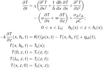
where x is the thermal diffusivity (1:12 x 10∼6 m2 s−1), C is the heat capacity, μ( x,t ) is air temperature, 0( t ) is the effective energy-exchange coefficient (Reference Paterson and ClarkePaterson and Clarke, 1978), q eff ( t ) is the heat flux released due to meltwater refreezing, Tb is temperature at the glacier bottom and T0 is the initial temperature in the ice. (We use the conventional summation notation for tensors.)
At x = 0 and x = L0 the boundary temperatures T 1 (z, t ) and T2{z, t) were taken from solution of the following auxiliary problems:

3. Method
Calculation of velocities is based on the diagnostic system (Equation (6)) at each time-step using temperatures calculated using the set of Equations (8). The new location of the surface, hs, is calculated from the mass-balance equation (7), and then temperatures are calculated at each new time-step.
The solution of the non-linear system of equations is determined by an iteration procedure in variables x=(hs − z)/H and x (Pattyn, Reference Pattyn2000). It allows us to transform the complex cross-section occupied by the glacier in a rectangular region II={0 x L}. In these variables the diagnostic system is

We have developed the finite-difference code GregFlow of these equations with first-order approximation in boundary nodes, and the second-order approximation in the internal nodes (Reference FletcherFletcher, 1991). A similar approach is used for the heat problem (Equation (8)).
4. Approximation of the Boundary Condition At the Surface
The boundary condition at the free surface was combined with Equation (2) to be consistent in the neighboring nodes. Computer tests show that it allows the number of iterations and the number of nodes in the vertical direction to achieve the needed accuracy to be reduced.
5. The Input Data
The term a 0 in Equation (7) is the difference between precipitation a 1 and ablation rate a 2, that is, the amount of meltwater runoff in summer months. Precipitation and ablation were approximated by linear functions of elevation, hs(x):

where n is a current year, t is time in years, ![]() , and a(t) is precipitation at 4100 m elevation, equal to that at the Tien Shan meteorological station (Fig. 2).
, and a(t) is precipitation at 4100 m elevation, equal to that at the Tien Shan meteorological station (Fig. 2).

Fig. 2. Precipitation at the Tien Shan station.
The coefficients in Equations (9) are determined by comparison of the balance a0 = a1 — a 2 to the average value measured in 1987 and 1988 (Reference MikhalenkoMikhalenko, 1989; Reference DjurgerovDjurgerov and others, 1995) (Fig. 3).

Fig. 3. Surface mass balance on the Gregoriev ice cap.
Air temperatures μ(x,t) are based on data at the Tien Shan meteorological station (Reference Arkhipov, Mikhalenko, Kunakhovich, Dikikh and NagornovArkhipov and others, 2004) (Fig. 4). The change of temperature with elevation for this region is 0.233˚C by 100 m (Reference MakarevichMakarevich and others, 1969):
where h0 is the elevation of the Tien Shan meteorological station (3615 ma.s.l.).

Fig. 4. Monthly average air temperature at the Tien Shan station.
6. Results
6.1. Evolution of the Gregoriev ice cap
The calculations show that the velocity in ice varies from 0 to 3 m a−1 along the glacier flowline. The maximum velocity is shifted from the lowest part towards the middle part of the Gregoriev ice cap for the studied period 1980–2050. The flow velocity near the front of the glacier is decreased for two reasons. The first is negative mass balance that results in thinning of the glacier tongue. The second is connected with deeper penetration of cold temperatures from the surface to the bed because of thinning of the glacier in its lower part. As a result, the internal heating becomes smaller in this part of the glacier and moderates the flow.
The changes of shape of the surface are mainly determined by the mass balance at the surface. At the surface at elevations h > 4400 m the mass balance is positive, which corresponds to observations (Reference MikhalenkoMikhalenko, 1989). At h < 4400 m, negative mass balance at the surface occurs. Near the glacier front, there is strong thinning and decrease in glacier length at a rate of ≈ 0:5 ma−1, which increases with time. Figure 5 compares the cross-section of the Gregoriev ice cap in 1980 (Fig. 5a) with that forecast for 2050 (Fig. 5b) assuming that air-temperature and precipitation trends will remain the same in the future as they were in 1930−2000.

Fig. 5. Horizontal velocity in the Gregoriev ice cap: (σ) in 1980; and (b) forecast for 2050.
6.2. Seasonal changes of temperature, stresses and velocities in subsurface layer of Gregoriev glacier
The borehole temperatures at hs ≈ 4600 m were measured in the borehole in 2003 and calculated for the same time (Fig. 6). The calculations were done with a time-step of 1 month. The calculated temperatures for each month in 2003 are shown in Figure 7.

Fig. 6. Observed and calculated temperature profiles in the Gregoriev ice cap.

Fig. 7. Calculated temperature profiles at x ≈ 0:18 km from the summit.
The heat source q eff(0 results in intense heating of the subsurface of the glacier in July and August (Fig. 7). The zero temperature front propagates down to 8 m depth. Seasonal changes of temperature induce variation of the viscosity in the subsurface layers (Fig. 8). A decrease of ice temperature from 0˚C to −20˚C causes variation of the coefficient A(T) in a range from 6:8 x 10∼15 to 1:7 x 10∼16 s−1 kPa−3. The viscosity 7] increases 3.5 times. Outside the layer of seasonal temperature changes (z>15m), there is practically no change in viscosity (Fig. 8).

Fig. 8. Viscosity profiles at x RJ 0:18 km from the summit.
Seasonal oscillations of the stress deviator follow the changes of viscosity (Fig. 9a). In winter months, changes of the stress deviator ![]() can exceed the strength of ice (≈102kPa), which can result in crack formation in the subsurface layers (Figs 9b and 10).
can exceed the strength of ice (≈102kPa), which can result in crack formation in the subsurface layers (Figs 9b and 10).

Fig. 9. Longitudinal stress deviator profiles ![]() (σ) and the longitudinal stress deviator at different depths (b) at x≈ 0:18 km from the summit.
(σ) and the longitudinal stress deviator at different depths (b) at x≈ 0:18 km from the summit.

Fig. 10. Longitudinal stress deviator ![]() at the surface.
at the surface.
The flow velocity changes in accordance with changes in the glacier slope. At 0 < x < 2:2 km, the slope increases with time, and the velocity increases also. At x > 2:5 km, the slope, ice velocity and ice thickness decrease (Fig. 11).

Fig. 11. Ice-thickness changes at some distances from the summit.
The influence of the term ![]() in Equation (2) on the solution increases with the slope of the glacier. For the Gregoriev ice cap, accounting for this term results in 5% difference of the numerical solution that is compared with input of the other integral term in Equation (2).
in Equation (2) on the solution increases with the slope of the glacier. For the Gregoriev ice cap, accounting for this term results in 5% difference of the numerical solution that is compared with input of the other integral term in Equation (2).
7. Conclusion
The thermodynamic state of the Gregoriev ice cap was studied by mathematical modeling. The observed data on the mass balance of the glacier, its surface shape and meteorological data (precipitation and air temperatures) were used as input to the model. For the time interval considered in this study, 1980−2050, the maximum velocity shifts from the lowest part toward the middle part of the Gregoriev ice cap. The ice velocity varies from 0 to 3 m a−1 along the glacier flowline, and the flow velocity near the front of the glacier is decreased. Seasonal variations of temperature result in changes of viscosity of ice, and, as a consequence, significant additional longitudinal deviatoric stress arises in places where the surface slope has large gradients. The resulting stresses can exceed the strength of the ice and result in crack formation. The derived changes of the glacier shape show the degradation and decrease of glacier extent on the south slope of Terskey Ala Tau.
Acknowledgement
This work was supported by the International Science and Technology Center (grant 2947).


