


Introduction
The objective of the work described here is to deduce topographical parameters for the bottom surface of a floating ice mass near the region of its grounding using synthetic aperture radar (SAR) imagery. The basic principles of SARs have been published in numerous papers and books (e.g. Reference HargerHarger, 1970; Reference KovalyKovaly, 1978) and the reader is referred to them for further information. The SAR is essentially a sideways looking radar, whose antenna bore-sight is, in this case, pointed in the across-track direction, and inclined at 45° to the vertical. The SAR thus views the bottom surface obliquely. The echoes received by the SAR are processed to give a two-dimensional image of signal back-scatter from the bottom surface. Musil (unpublished) and Reference Musil and DoakeMusil and Doake (1987) previously presented such images obtained from the bottom surface of floating ice near the region of its grounding. A more detailed analysis of these results will be attempted here. Both the spatial and amplitude information of the resolved echo amplitudes in the SAR images will be used to show that underside scarring of floating ice is likely to be present. Such scarring would be introduced at the point of grounding and be in the form of a drawn-out imprint of the bedrock surface.
Type of Signal Back-Scatter Expected in the Antarctic When Using a Sar
The SAR used was sledge-mounted and, although signal refraction at the air/ice surface and within the firn layer bends the signal rays closer to the vertical, the angle of signal incidence at the assumed horizontal bedrock surface lies in the range of 14-31° (typically 22°). Using a standard RE sounder, whose antenna points vertically downwards, Oswald (unpublished) has shown that the bedrock surface typically encountered in the Antarctic can be treated as a collection of randomly orientated facets whose size is greater than the wavelength in ice of a 60 MHz radar signal. One would therefore expect that the 120 MHz SAR used by Reference Musil and DoakeMusil and Doake (1987) would only register a specular type of signal back-scatter from the bedrock surface with slopes in excess of 14°, so that some of its facets face normally the incoming radar signal. From his measurements in East Antarctica, Oswald (unpublished) concluded that the r.m.s. slope of the surface facets is less than 10° and typically 2.5°. He also concluded that the vertical scale of the bottom irregularities is greater than 0.3 m. Similar results were also reported by Reference WagerWager (1982) for Spartan Glacier (Alexander Island), by Reference Walford, Kennett and HolmlundWalford and others (1986) for a sub-polar glacier in Sweden, and by Reference NealNeal (1982) for the bottom surface of Ross Ice Shelf.
The above authors used radar antennae whose bore-sights pointed vertically downwards into the ice. From their measurements, at the low bedrock slopes, they were able to assume that diffraction of the radar signal did not make a significant contribution to the received echoes. The same, however, cannot be said of the echoes received when using a SAR. From the above results, it appears that the side-looking nature of the SAR would result in the specular signal reflections being directed away from the SAR antenna. One can therefore conclude that, with the exception of regions of significant geography such as sides of valleys, etc., the signal back-scatter for a 120 MHz SAR is most likely to be the result of signal diffraction for the bottom surfaces generally encountered in the Antarctic.
Reference Musil and DoakeMusil and Doake (1987) further noted that virtually no speckle was present in their SAR images, which are made up of pixels each corresponding to an area of 8 m x 8 m of the bedrock surface. This, together with the independent observations made by Oswald that the sizes of bedrock facets are greater than about 3 m, allows one to make a reasonable assumption that, for the most part, the resolved echo signal of each image pixel corresponds to back-scatter from one dominant facet. It shall also be assumed that the subglacial back-scattering surface is undulating with slopes no greater than 10°, that it contains no cracks nor large boulders, and that it has a uniform reflection coefficient.
Signal Diffraction From a Randomly Orientated Facet
Before the echo-amplitude information contained in the SAR images can be related to the physical nature of the bottom surface, the signal back-scatter of the individual facets, which make up the surface, must first be understood.
Consider a randomly orientated square facet of side a (m), inclined β° to the horizontal, and rotated ϕ°0 in azimuth (see Fig. 1). It is assumed that the height of the radar antenna above the ice surface is very much smaller than the ice thickness R0. It is also assumed that the ice is lossless and that it has a constant refractive index. The angle of signal incidence at the assumed flat surface of the facet is θ′°. If the transmitter (Tx) and the receiver (Rx) share the same antenna, and the facet lies in its far field, then the electric field Es at the facet surface is

where E0 is the signal transmitted by the radar at range R and λ is the signal wavelength in ice. The electric field ER

Fig. 1. Geometry of a randomly orientated facet used in deriving the amount of signal back-scatter. (Negative values of β referred to in the text correspond to 180° rotation of the facet in azimuth, i.e. in Figure 1 the facet would then be inclined towards rather than away from TX RX.) β is facet inclination to the vertical (z) direction, Q0 is azimuthal orientation of the facet, Q is azimuthal orientation of the facet when referred to the radar position, R0 is ice thickness, |R| is radar range of the facet, and θ′ is angle subtended by the facet normal (N) and the signal ray.
scattered by the facet back to the receiver antenna is

where ρ� is the effective surface-reflection coefficient and ρdEs is the electric field re-radiated by a point source on the facet surface. By changing the variables, Equation (2) becomes


Fig. 2. Calculated echo amplitude plotted as a function of radar position along the synthetic aperture for various facet sizes. The synthetic aperture is 104 m long. The facet is inclined at 8° to the horizontal and is orientated at 23 in azimuth.
where x0 and y0 are the x and y coordinates at the centre of the facet and xT is the position of the radar along the synthetic aperture. Equation (3) can be numerically integrated for any facet size and orientation. Figure 2 shows the effect of facet size on the echo amplitude as the radar moves along the synthetic aperture. Returns from facets of sides 4, 5, and 6 m are shown. The facets are inclined at 8° to the horizontal and are orientated at ϕ0 = 23° in azimuth. Using the geometry defined in Figure 1, the centres of the facets are located at (52, 72, 0 m), and the radar moves along the line ϕ = R0, y = 0, where R0 = 290 m. The signal wavelength in ice of the 120 MHz SAR is close to 1.4 m. Figure 2 shows that, as the facet increases in size, signal scattering from it becomes more specular. This is manifested as a decrease in signal back-scatter for increasingly larger facets when, as in this case, the facets are not viewed normally. It can also be seen in Figure 2 that the scattering of the radar signal becomes more diffuse for smaller facets. This is shown by the wider separation of echo minima for the smaller facets, thus making the echo amplitudes less dependent on the radar position along the synthetic aperture.
Figure 3 shows the received echo amplitudes along the synthetic aperture for a facet 5 m x 5 m in size, and which is orientated at ϕ0 = 143° in azimuth. The three curves correspond to facet inclinations of −8°, 0°, and +8°. Figure 3 shows the general tendency for the aperture-averaged amplitude of the echo signals to decrease with increasing aperture-averaged angle of signal incidence θ′AV. The values of θ′AV are 10.3°, 15.0°, and 21.6° for facet inclinations of −8, 0°, and +8°, respectively.
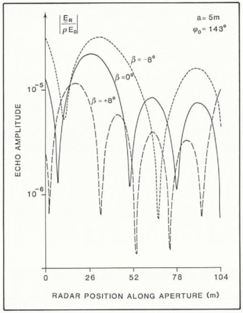
Fig. 3. Calculated echo amplitude plotted as a function of radar position along the synthetic aperture for various facet slopes. The square facet has a side of 5 m and is orientated at 143° in azimuth.
It should be noted that, in deriving Equation (3), it was assumed that the signal back-scatter was not limited by the transmitted pulse length. This effectively limits the usefulness of Equation (3) to facets which are smaller than the resolution capability of the SAR (i.e. about 8 m x 8 m in this case).
It therefore appears that even relatively small bedrock facets, whose dimensions are not very much greater than the signal wavelength in ice, should produce meaningful signal back-scatter from which parameters for the bedrock topography can be interpreted. The SAR images could therefore contain information about the groove-like features which are thought to be present on the underside of floating ice sheets.
Determination of the Periodicity of The Underside Scarring
It has been previously suggested that an ice mass, flowing across a grounding line, retains a drawn-out imprint on its bottom surface of the bedrock undulations at which the ice was last grounded. That is, the underside of floating ice will have groove-like scarring which runs along the direction of ice flow, and which is representative of the two-dimensional roughness of the bedrock surface along the line of grounding. It should be noted that the true line of grounding is likely to be subject to tidal migration. The bedrock surface in the region of grounding is also likely to have a top layer of deformable, melted-out debris, as most sedimentation occurs close to the grounding line (Reference Drewry and CooperDrewry and Cooper, 1981; Reference Orheim and ElverhoiOrheim and Elverhoi, 1981). The grounding line referred to here is therefore that part of the bedrock which is responsible for scarring the bottom ice surface. The measure of surface roughness is defined as the ratio of amplitude to wavelength (Reference HalletHallet, 1981). Although it is possible that this two-dimensional roughness of the bedrock surface may not be equal to that of the underside of the floating ice sheet some distance away from the grounding line, it is assumed here that bottom melting or freezing will not significantly alter the period of bottom scarring. It may have a smoothing effect by reducing the amplitude of the scarring.
The above analysis indicates that such grooving would be manifested in the SAR images as a periodic variation in the level of the resolved signal back-scatter. This is because facets of the grooved topography would face slightly towards and then away from the observer in a periodic fashion. By taking a Fourier transform in the spatial domain of the imaged echo amplitudes, the dominant wavelengths of the underside irregularities should become identifiable. Such a spatial Fourier transformation can be written in discrete form as

where |F(T)| is the amplitude of sinusoidal undulation with a period of Τ m which is present in the echo data of the image, and A(k) is the echo amplitude of the kth image pixel. The centres of the image pixels are separated by #x03B4;xm.
The derived theoretical relationship between a surface facet and the back-scatter received from it can now be used to look at the SAR images obtained by Musil and Doake (1987) from the underside of Bach Ice Shelf. The extent of the imaged areas is as shown in Figure 4. The direction of ice flow (deduced from the results of the above authors) and the region of ice grounding are also shown. Fourier transformation defined by Equation (8) was applied to the strings B-B′ and E-E′ of the image pixels in images AA-BB and EE-FF. The result is shown in Figure 5. It appears that both images contain one spatial wavelength which is dominant. The dominant undulations in the image AA-BB have a period of 24.7 m when viewed along the direction of B-B′, whilst those of image EE-FF have a period of 37.8 m along E-E′. If the periods of these dominant undulations correspond to subglacial scarring which runs along the direction of ice flow, then the dominant period, TD, of such scarring must satisfy the relation
for #x03D5;AB = 143°(37°) and #x03D5;EF = 23° where TAB, TEF, and #x03D5;AB, #x03D5;EF are the dominant periods of variations in the echo amplitudes and the angles of azimuthal orientations of lines B-B′ and E.E′, respectively. Taking #x03D5;AB and #x03D5;EF to equal 143° and 23° as is shown in Figure 4, then from data B-B′ of image AA-BB TD = 14.9 m, and from data of image EE-FF TD = 14.8 m.
The above results support the proposition that the bottom surface of floating ice contains groove-like scarring in the vicinity of a grounding line, and that such scarring runs in the direction of ice flow. It is expected that, in the vicinity of the grounding line, roughness of the bedrock surface in a direction perpendicular to ice flow has the same dominant period of about 14.8 m.
Estimating Size of Facets Making up the Bottom Surface
The relationship between the spatial distribution and the level of signal back-scatter contained in the image pixels was used above to derive the dominant period of the subglacial scarring. The ratio of the maximum to minimum levels of signal back-scatter are now used to estimate the size and the maximum inclination of the dominant surface facets.

Fig. 4. Physical extent of the subglacial, imaged areas on Bach Ice Shelf and their orientation relative to the direction of ice flow. The strings of image pixels marked B-B′ and E-E′ are used in the analysis of surface roughness.

Fig. 5. The left-hand graphs show the relative echo amplitudes of the groups of image pixels shown in Figure 4. The right-hand graphs show the result of Fourier transformation in spatial domain. Separation of the centres of adjacent image pixels is equivalent to 8 m on the ground.
Using Equation (3), the aperture-averaged echo amplitude, A, which corresponds to the level of signal back-scatter in any one image pixel is of the form

where N is the number of sounding points along the aperture, and M is the total number of facets contained in an area of bottom surface corresponding to one image pixel. If, as is reasoned above, it is reasonable to assume that only one dominant facet is present, then

If the bottom surface contains linear scarring, then adjacent pixels in an image that views the grooves obliquely should exhibit some form of periodic variation in their brightness. The ratio of the maximum to minimum amplitudes of such variation can be written as

If the facet size and its orientation are known, then the above fraction can be evaluated using Equation (3), provided the conditions for maximum and minimum echo returns are known. It was shown above that, in general, stronger signal back-scatter is expected from those facets at which the angle of signal incidence is the smallest over the whole of the synthetic aperture. For a fixed facet size, a, and its azimuth orientation, ϕ0, the maximum and minimum levels of signal back-scatter will thus be determined by the facet inclination, β For a sinusoidally corrugated surface, β will oscillate between some peak positive and negative values. Thus, the bottom scarring of roughness less than 0.04 (i.e. surface slopes less than 14), the aperture-averaged values of the maximum signal back-scatter would, to a first degree of approximation, occur when
β= maximum and +ve, (when ϕ0 = 143°) for image AA-BB,
β = maximum and -ve, (when ϕ0 = 23°) for image EE-FF.
Similarly, minimum level of signal back-scatter would occur when
β = maximum and +ve, (whenϕ=143°) for image AA-BB,
β = maximum and -ve, (when ϕ0 = 23 ) for image EE-FF.
If it can be assumed that the bottom-reflecting surface contains predominantly linear, sinusodal corrugations, then the above quantity of Equation (12) can be measured directly from the variation in the brightness of the SAR images. From the previous section, this can be achieved using

where F(TD) is the amplitude of the dominant sinusoidal corrugations and F(∞) is that of corrugations having an infinite period (i.e. the mean value). By applying the above Equation (13) to the data shown in Figure 5 for the images AA-BB and EE-FF, then

Fig. 6. Plot of the calculated, aperture-averaged, echo amplitudes as a function of facet slope. The side of the square facet is 4 m in size. Plots for two azimuthal orientations of the facet are shown.

These results, which come from two independent images of the same, predominantly corrugated surface, can be equated to the theoretical results of Equation (12). We thus have two equations, one for image AA-BB in which ϕ0 = 143° and one for image EE-FF in which ϕ0 = 23°, with two unknowns: the facet size, a, and the maximum slope β0. It is therefore possible to derive the size of the surface facets which are dominant in the signal back-scatter.
Figure 6 shows the aperture-averaged echo amplitudes received from square facets (of side 4 m) plotted against the facet slope β. The two curves correspond to facets which are rotated through 23° and 143° in the azimuth. For ϕ0 = 143°, the ratio of maximum/minimum echo amplitude of 1.48 (see Equations (14)) is satisfied when β0 = ±3°. For ϕ0 = 23°, the ratio of maximumyminimum echo amplitude of 1.37 occurs when β0 = ±4.5. Since the echo signals originate from a common subglacial surface, the values of β0; should be equal. To find the size of surface facets which satisfy this, β0 is evaluated for several facet sizes. By plotting the results, common values for β0 and facet size can be found from the point where the two curves meet. From Figure 7, the maximum slope of the facets making up the subglacial surface is near 5.4° and the sides of the assumed square facets are about 4.5 m in size. It is not, however, clear from Figure 7 whether this is the only solution to the above problem. One would expect the value of β0 to decrease as the size of the facet increases. However, since the SAR images are of the ice underside very close to the grounding line, it is reasonable to expect the bottom-surface slopes to be more comparable to those of the bedrock surface rather than to the smoothed outer parts of the floating ice shelf (i.e. one would expect a higher, rather than lower, value for β0). The values for β0 and a derived above seem therefore to be the most appropriate.

Fig. 7. Plot of the maximum facet inclination ( β0) as a function of facet size (a) for the two orientations in azimuth.
Vertical Extent of Underside Scarring
In deriving the effective sizes of facets making up the bottom surface, their maximum inclination to the horizontal, β0, was also derived. Using this result, the amplitude h0 of the dominant sinusoidal component of the underside scarring of the ice mass can be simply evaluated as

If the dominant sinusoidal component of the subglacial scarring is representative of the overall bottom-surface roughness, the bottom of Bach Ice Shelf, near its line of grounding, has a roughness across the line of ice flow of 0.015, justifying the initial assumption of a roughness of less than 0.04 (which corresponds to β0 < 14°).
Conclusions
From analysis of SAR imagery, it appears that the bottom surface of Bach Ice Shelf does contain linear scarring which runs in the direction of ice flow. Using Fourier analysis, these scars were shown to contain a dominant sinusoidal component with roughness parameters as follows:
Period of subglacial scarring = 14.8 m, Amplitude of scarring = 0.22 m, Maximum surface slope = 5.4°, Equivalent size of square facets making up the bottom surface = 4.5 m, Direction of scarring = 53° with image AA-BB, and 67 with image EE-FF.
These results are consistent with those obtained by other authors (see beginning of this paper) at different sites. It is therefore very probable that the roughness parameters, measured by, for example Reference NealNeal, (1982) at the bottom surface of Ross Ice Shelf, correspond to subglacial scarring rather than a randomly roughened surface. Since the roughness parameters of a typical bedrock surface (Oswald, unpublished) are very similar to those derived above for the underside of floating ice in the vicinity of its grounding, we assume that such scarring is introduced in the region of grounding. It is expected that such scarring on the bottom of ice shelves would, in time, be smoothed out due to spreading out of the flowing ice mass, and possibly due to melting/freezing at the bottom surface. Evidence of such smoothing can be seen in the results of Neal (1982) which show a marked decrease in bottom-surface roughness at the outer parts of Ross Ice Shelf.
If scarring is preserved and found to be present at the outer parts of floating ice sheets, it could be used to trace the sources of the ice found at the calving edge of the floating ice sheet.
Acknowledgements
I am grateful to the British Antarctic Survey and to Dr C.S.M. Doake for allowing me to use the results of their SAR survey on Alexander Island. I am also indebted to Dr I. Allison and Dr K. Echelmeyer for helpful reviews which led to substantial improvements in this paper.


