


Introduction
The amounts and processes of snowmelt at high elevation are crucial to modelling summer inflows to hydroelectricity storage lakes in New Zealand. Even though hydropower generates >60% of total electricity in the country, snowmelt at high elevation has not previously been investigated. Snowmelt runoff estimates are needed for forecasting seasonal water yields, river regulation, reservoir operation, and determination of design floods. The aim of this paper is to address this deficiency by assessing the validity of the degree-day model of snowmelt at an alpine site within the highest catchment of the Southern Alps (Fig. 1).

Fig. 1. Location of the study site, showing the main divide of the Southern Alps, Tasman Glacier and Lake Pukaki.
In most cases, snowmelt is estimated using either the energy-balance approach, or a temperature-index method such as the degree-day model. An energy-balance method requires information on radiation energy, sensible and latent heat, energy transferred through rainfall onto the snow and heat conduction from the ground to the snowpack. Often such information is not available, especially for high alpine areas, so the temperature-index method is considered the best substitute for the energy balance and is widely used (e.g. Reference Martinec and RangoMartinec and Rango, 1986; Reference Singh and SinghSingh and Singh, 2001; Reference Lefebre, Gallee, van Ypersele and HuybrechtsLefebre and others, 2002).
The degree-day model uses a simple temperature index to calculate snowmelt:
where M is daily snowmelt (in mmw.e.), f is a degree-day factor (mm ˚C–1 d–1), T a is the average daily air temperature (˚C), T b is the base temperature (0˚C for snow), and T a – T b is number of degree-days (˚C–1 d–1) for T a > 0˚C.
The degree-day model offers the advantage of simplicity because it only requires temperature as input, which is often readily available, or it can be lapsed from nearby climate stations. Observations in the European Alps, Scandinavia and Greenland show a strong correlation between melt rates and f (Reference Braithwaite, Olesen and OerlemansBraithwaite and Olesen, 1989; Reference Braithwaite and ZhangBraithwaite and Zhang, 2000). However, f can vary over time and from place to place, so that field studies are needed to determine its value in each catchment. Another issue is estimation of high-elevation temperatures using data from valley climate stations: several authors have found that lapse rates need not be constant and can vary from glacier to glacier and by synoptic weather patterns (e.g. Reference BarringerBarringer, 1989; Reference Greuell and BöhmGreuell and Böhm, 1998).
For the purposes of hydrological modelling, normal practice is to choose a value of f based on the season, state of the snow and on previous experience. A wide range of 0.7–9.2mm˚C–1 d–1 has been reported in literature (Reference Singh and SinghSingh and Singh, 2001), but values of f are generally in the range 3.5–6.0mm˚C–1 d–1 according to Reference Martinec and RangoMartinec and Rango (1986). They state that f tends to increase with increasing snowpack density. Other key factors are an increase in the amount of incoming solar radiation and a decrease in the albedo of the snow surface as the melt season progresses. Seasonal variations in other meteorological variables, such as the vapour pressure of the air, wind speed and cloud cover, also influence f. Reference BraithwaiteBraithwaite (1985), Reference Braithwaite, Olesen and OerlemansBraithwaite and Olesen (1989) and Reference ReehReeh (1991) tested degree-day models under Greenland conditions and found marked variations in f. Reference Braithwaite, Olesen and OerlemansBraithwaite and Olesen (1989) attempted to explain these in terms of the energy balance, while Braithwaite and Zhang (2000) indicate that the reasons for variations in f are not always immediately obvious. In the Swiss Alps at 2600ma.s.l., Reference Plüss and MazzoniPlüss and Mazzoni (1994) found that the energy-balance model seems to perform better on a daily basis, but that the degree-day model worked well over longer periods. They argue that the degree-day model tends to significantly underestimate measured melt, largely because it relates more to the sensible-heat flux component rather than other fluxes of the energy balance. On the other hand, Reference OhmuraOhmura (2001) argues that the simple degree-day model works well because of the close relationship between incoming longwave radiation and temperature. Reference Zuzel and CoxZuzel and Cox (1975) considered that when there is a significant change in air mass, air temperatures near the surface are a poorer index of snowmelt and the degree-day model is less satisfactory than during relatively stable weather periods.
Within the New Zealand context, snowmelt has been measured (e.g. Reference Moore and OwensMoore and Owens, 1984a, Reference Moore and Owensb; Reference BarringerBarringer, 1989) and the degree-day model tested with some success, but there have been no measurements above 1800ma.s.l. Reference Fitzharris and GarrFitzharris and Garr (1995) used a degree-day model for daily calculations of snowmelt within their SnowSim model, which provided reasonable estimates of water stored as seasonal snow within the main hydroelectricity catchments of the South Island. A major difficulty for the modelling lay in the choice of f, especially at high elevations in summer for which no data were available. Reference Woo and FitzharrisWoo and Fitzharris (1992), when modelling mass balance on Franz Josef Glacier, New Zealand, introduced a variable f to account for decreasing surface albedo of snow as it aged and for the effects of rain-on-snow events. These adjustments improved model output further, when tested against measured data, but errors increased above 1950ma.s.l., possibly because of errors in estimating snowmelt. Assessments of f on lower Tasman Glacier (960 and 1360ma.s.l.) are available from Reference KirkbrideKirkbride (1995), but there are none for sites above the equilibrium-line altitude (ELA). Reference Neale and FitzharrisNeale and Fitzharris (1997) tested the degree-day model against measured snowmelt at Mueller Hut (elevation 1780 m), elsewhere in the Pukaki catchment of the Southern Alps (Fig. 1). They found that that the degree-day model generally worked well, except during northwesterly storms, when melt rates were seriously underestimated. They recommended that the behaviour of f be investigated further at higher elevations and under different synoptic weather conditions.
Study Area
Snowmelt and associated meteorological variables were measured within the Pukaki catchment (at 2440ma.s.l. on upper Tasman Glacier), which is >500m above the glacier ELA. The study site is shown in Figure 1, and lies in the heart of the Southern Alps about 2 km east of the main divide, which trends across the prevailing mid-latitude westerly winds of the Southern Hemisphere. It has a slope angle of <10° and is orientated towards the southwest. Even though located on a glacier, the surface at the study site consists of snow deposited during the previous winter and spring. The site is always snow-covered, and bare ice is never exposed here. The depth to glacier ice is unknown, but based on observations in crevasses is in the order of tens of metres below the surface.
Anticyclones and depressions cross the mountains from west to east as a series of synoptic waves. Precipitation at the study site is estimated at >6000mma–1, so seasonal snow accumulation is very deep. Most precipitation occurs as spillover from the west, and leads to a strong gradient away from the main divide (Reference Griffiths and McSaveneyGriffiths and McSaveney, 1983). Even though high in the mountains, the site is considered maritime in character, being <30km from the Tasman Sea to the west.
The Pukaki catchment drains the highest part of the Southern Alps, and ranges in elevation from 500m to >3700 m. Snowmelt is an important source of water for supplying spring and summer river flow for the seven hydroelectricity-generating plants downstream of this catchment; together these can produce almost 2000 MW, or about 40% of New Zealand’s generating capacity. From Reference Fitzharris and GarrFitzharris and Garr (1995), it is estimated that about half of the inflows to Lake Pukaki during November–February are from melt of seasonal snow. This compares with the contribution from glacier melt of about 10%, despite the fact that the catchment contains the very large Tasman and other glaciers. Ice melt at lower elevations has been described by others (e.g. Reference KirkbrideKirkbride, 1995; Reference Purdie and FitzharrisPurdie and Fitzharris, 1999) and is much better understood. This paper concentrates on melt of seasonal snow at high elevation on the glacier. Along with rainfall, it is the more important contributor to inflows to local hydro lakes over the spring and summer months.
Methods
All measurements were made over a 34 day summer period (19 January–22 February 2001). This period included a diverse range of weather conditions, but was generally typical of summer conditions. The seasonality of snowmelt at elevation 2440m is not well known, but based on an analysis of atmospheric freezing levels, most is probably confined to the period from mid-December to mid-March. A first measurement of snowmelt (M l) was made using a lysimeter, which is a Perspex tray of dimension 0.53 m by 0.36m located at 0.6–0.8m depth beneath the snow surface. The tray was inserted horizontally into undisturbed snow from an adjacent trench, which was then back-filled. The bottom of the tray drained to an electronic tipping-bucket mechanism, housed in an insulated box beneath. The number of tips was totalled at half-hourly intervals by a Campbell CR21X scientific logger and converted to water readings (mm depth). Data were adjusted by 5 hours, the percolation lag time between the surface and the lysimeter that was typically observed at this site. The 5 hour time shift is the time it takes for the water to get from the snow surface to the depth of the lysimeter, and was determined by comparing the time of peak water flow from the lysimeter with the time of peak energy availability for melt. Measurements of rainfall were subtracted from the lysimeter readings to give snowmelt totalled for a 24 hour calendar day. The rain gauge was checked twice daily. It was maintained at a level such that the orifice was approximately level with the snow surface and surrounded by a grid wind shield of area 1 m2 constructed from white plastic. New snowfall (water equivalent) was calculated from daily observations of depth on a surface snow board and measurements of new snow density.
A second measurement of snowmelt (M s) was obtained from an array of ten ablation stakes. These have the advantage over the lysimeter that they cover a wider spatial area of about 40 m2 and directly measure the melt at the snow surface without recourse to a lag time. The stakes consisted of 0.025m thick PVC tubing of length 2.0 m. Changes in snow depth were observed near sunset every day, and when coupled with daily manual measurements of snow density from the upper 0.5 m of the snowpack at each stake, give the snowmelt in mmw.e. Loss of snow by evaporation is considered negligible in this strongly maritime environment. Data at all ten stakes are averaged to give daily values of M s.
Air temperature at the study site was measured at an average height 1.5 m above the snow surface as part of a solar-powered automatic climate station. The station was checked at least daily. The instrument was an aspirated platinum resistance thermometer placed inside a tubular radiation shield constructed of PVC piping lined with insulation (Armaflex) and covered externally with aluminized mylar reflective tape. The aspiration rate was approximately 4 ms–1. Temperature output is logged every 5 s, then averaged at half-hourly intervals. Mean temperature is calculated daily from these data to obtain T a. Snow temperatures were measured using an array of thermocouples at depths of 0.07, 0.2, 0.35, 0.5 and 1.0 m and were logged at 30 min intervals.
Comparison of M l and M s shows strong correlation within a linear relationship (M s = 0.8M l with correlation coefficient r = 0.87), so these values are averaged for each day to obtain combined measured melt (M c). Values of M c are plotted against (T a V T b). The validity of the degree-day model was judged by visual inspection of any linear relationship and the value of r. As based on a rearrangement of Equation (1), f is given by the slope of best-fit linear regression.
Errors
The total error in snowmelt measurement is difficult to precisely quantify, but is reduced by application of two independent sets of measurement, by regular field maintenance and by calibration of instruments. The lysimeter tipping-bucket mechanism demonstrates 1 : 1 linearity with measured flow rates up to at least 240 mm min–1 and has an estimated error of ±3% (Reference CampbellCampbell, 1987). The method assumes that all meltwater at the snow surface finds its way into the lysimeter; it is possible some may refreeze in the layer between it and the snow surface, or some may move horizontally at ice layers above the lysimeter, and not be trapped by it. Temperature sensors in the upper metre of the snowpack indicated isothermal conditions at 0˚C for most of the measurement period, except for the upper 0.2 m during some nights and on five of the days. Other possible measurement errors arise from tilting of the lysimeter within the snowpack causing spill-out of meltwater, and freezing of meltwater in the drainage tube between the lysimeter and the tipping-bucket mechanism. Errors may also arise from any under-catch of the rain gauge in strong winds. It is difficult to quantify these errors, but they are probably about ±15%.
Underestimation of snowmelt can occur with ablation stakes, due to their possible subsidence within the snow during strong winds and high radiation days. M s values on average tend to underestimate M l by 0.8. At least half of each stake was inserted below the snow surface, following the recommendation of Reference Griffiths and McSaveneyLaChapelle (1959) to minimize stake subsidence. Reference ChinnChinn (1969) in an early study on Tasman Glacier assumed an error of ±20% for individual stakes. Since M s is an average of ten stake readings, errors will be less than this and are estimated at ±10%. Stake readings were taken near sunset, but assigned to that 24 hour calendar day. This procedure assigns any nocturnal melt occurring up until 2400 NZDT (New Zealand Daylight Time) to the following day, whereas the lysimeter melt is for the actual 24 hour calendar day. However, this error is likely to be small, as the lysimeter showed that melt occurs as distinct diurnal pulse and that nocturnal melt is negligible on all but a few occasions. Laboratory tests of the temperature sensor against an electronic reference thermometer before and after fieldwork showed that T a is likely to be measured within ±0.2˚C. The height of 1.5 m above the snow surface varied during the period, depending on changes in level of the snow surface and settlement of the climate station, but was readjusted daily.
Results
Over the study period, air temperatures ranged from –8.2˚C to 10.8˚C, with a mean of 2.5˚C. Snow temperatures in the upper metre of the snowpack remained close to 0˚C, except for 17–26 January, when they sometimes fell to –2.0˚C, and in the upper 0.2 m, when they cooled to –1 to –2˚C on many nights. Snow density in surface snow increased from 480 kgm–3 to 550 kgm–3 over the study period. There were five distinct precipitation events (23, 25–26 and 31 January, and 5 and 15–16 February) with amounts ranging from 10 to 110 mmd–1. Most occurred as rain, with the only significant snowfall being 36 mmw.e. during the second event.
M l averaged 19.9 mmd–1 and varied from 0 to 119mmd–1. M s averaged 15.4 mmd–1 and varied from 0 to 55 mmd–1. M c averaged 17.8 mmd–1 and varied from 0 to 78 mmd–1. The differences between M l and M s were generally small, except during an intense melt event on 15 February, when 119mm was recorded by the lysimeter, but only 37 mm by the network of ablation stakes (Fig. 2).

Fig. 2. Daily snowmelt over the study period.
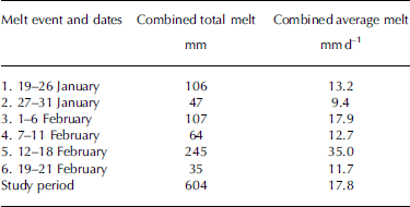
Over the measurement period, melt occurred in six distinct melt events, each lasting for 5–8 days (see Fig. 2, where the minimum in the melt curve marks the end of each event). Each melt event, or pulse, coincided with an approximate weekly synoptic cycle. The cycle began with an anticyclone advancing across the Tasman Sea following the passage of a trough, with associated cold, southwesterly winds over the Southern Alps. Winds eased as the high pressure dominated the area for 1 or 2 days and temperatures warmed. Eastward movement of the next trough and associated cold front across the Tasman Sea increased wind flow over the Southern Alps from the west or northwest. Typically the trough was accompanied by a further rise in temperature, an increase in humidity and rain. There was a drop in temperature with the passage of the cold front and a return to southwesterly winds and the beginning of the next cycle. A summary of snowmelt for each event is given in Table 1. Over the 34 day period, total melt was 604 mm. Average daily melt for each melt event varied considerably, from 9.4 mmd–1 for event 1 up to 35.0 mmd–1 for event 5. The latter accounted for over one-third of total melt for the measurement period.
Table 1. Combined melt for melt events and for the 34 day study period
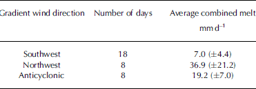
Lower-melt days coincide with snowfall, temperatures below freezing, and winds from the south. For example, on 26 January, M c = 0, while T a was <–4˚C for much of the day. Similarly on 31 January, M c = 0, while T a was <–1˚C for much of the day. Higher-melt days are those with rain, temperature above 5˚C, and storm events from the northwest. When snowmelt is classified by the direction of the gradient wind over the Southern Alps, as determined from daily synoptic maps of surface pressure patterns, there is a clear demarcation as shown in Table 2. Application of t tests shows that differences between these synoptic wind categories are significant at the 95% level of confidence. Average melt during northwest days is five times greater than that during southwest days, while that on anticyclonic days is over two times higher.
Table 2. Combined melt given as average daily values (±1 std dev.) according to the gradient wind direction over the Southern Alps
Daily values of M c are plotted against T a – T b in Figure 3 .Here, r = 0.70 and the slope of the best-fit linear regression line f = 4.9mm˚C–1 d–1. However, there are several obvious outliers on the plot, where values of M c are well above the best-fit line. Many of these are identified from daily synoptic maps as days of northwesterly flow over the Southern Alps and are shown as open circles. When the eight northwesterly days are removed from the data, the best-fit regression line has r = 0.94 and f = 3.4mm˚C–1 d–1. This suggests that the degree-day model is very satisfactory for all but northwest days. Either the latter require a much higher value of f, or an entirely different approach is required for them.

Fig. 3. Degree-day relationship for the study site. Combined measured melt plotted against melt degree-days. Line a is for all data, and line b is with northwesterly days (open circles) removed.
Discussion
There is a discrepancy between M l and Ms, with the ablation-stake method recording less snowmelt than the lysimeter. This is particularly marked on the largest-melt days. One possible reason is subsidence of stakes as the snow becomes soft and as they are jiggled by the strong gusty winds typical of northwesterly days. Alternatively, rainfall could be under-caught during high-elevation winds, which means the lysimeter melt is overestimated. Real surface melt is probably somewhere between M l and M s, hence the decision to combine them in this analysis.
Few authors provide values of maximum daily snowmelt. Reference Young and LewkowiczYoung and Lewkowicz (1990) measured 161 mmd–1 at an Arctic site. In New Zealand, Reference Moore and ProwseMoore and Prowse (1988) recorded 93 mmd–1 in the Craigieburn Ranges, and Reference Neale and FitzharrisNeale and Fitzharris (1997) reported 63 mmd–1 at Mueller Hut. Thus, maximum combined melt of 78 mmd–1 from the study site is not particularly unusual. However, these values are comparable to daily rainfall rates for moderate-size storms, and indicate that snowmelt can make significant contributions to summer river flows.
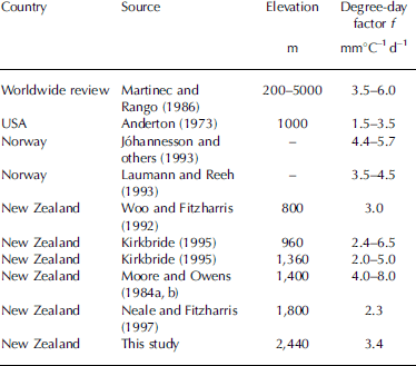
Temperature-index models provide simple-to-use mathematical formulae that are able to calculate daily totals of melt for various elevations within a catchment. The main aim of this paper was to determine f for snowmelt at high elevation, so as to be able to increase the predictive power of hydrological models in important hydroelectricity catchments. For example, the findings of this paper and of Reference Neale and FitzharrisNeale and Fitzharris (1997) have enabled improvements to the way f is parameterized within the SnowSim model. Table 3 presents a range of degree-day factors f for New Zealand and overseas. It needs to be recognized that the table is comparing sites with widely varying days of record and seasons. However, an f value of 3.4 mm˚C–1 d–1 for seasonal snow at the high-elevation study site is consistent with worldwide values of f and those for lower elevations on Tasman Glacier by Reference KirkbrideKirkbride (1995), but higher than the 2.3 mm ˚C–1 d–1 for seasonal snow calculated at 1780ma.s.l. at Mueller Hut by Reference Neale and FitzharrisNeale and Fitzharris (1997). Further work is required to evaluate the spatial variability of f for the Pukaki catchment. Values of f may also change from year to year. What is ultimately required is a dynamic procedure for determining f based on prevailing synoptic weather conditions.
Table 3. Sample of snowmelt degree-day factors
Snowmelt markedly increased during northwesterly conditions. Changes in weather patterns can influence the degree-day factor considerably. Calculation of a refined degree-day factor for northwest storm events has been attempted by Reference Neale and FitzharrisNeale and Fitzharris (1997). They also found that snowmelt was boosted in these events, so that a ‘super degree-day factor’ of 11.5 mm˚C–1 d–1 (or four times the usual value) was suggested, although only 2 days of such conditions were available for their analysis. In an attempt to further refine this ‘super degree-day factor’, their data of northwest events are combined with those here. The result is given in Figure 4. There remains considerable scatter (r = 0.79), but the slope of the best-fit line indicates f = 9.1mm˚C–1 d–1 for northwesterly days. This is almost three times the value for other weather conditions. A larger sample of such days is required to further examine this issue. A statistically robust correlation requires a sample size of at least 30, and it is not yet clear whether the relationship between melt and degree-days is even linear. However, the overall findings indicate that hydroelectricity managers can derive much useful information about likely snowmelt runoff into storage lakes from an examination of daily synoptic weather maps. These are readily available for New Zealand on the internet.

Fig. 4. Scatter plot showing the relationship between combined measured melt and melt degree-days for northwesterly melt events. Data points from Reference Neale and FitzharrisNeale and Fitzharris (1997) are included and are shown as stars.
Northwesterly days involve advection of a warm, moist air mass across the Tasman Sea, often from subtropical latitudes. As noted by Reference Neale and FitzharrisNeale and Fitzharris (1997), these days have higher than usual contributions to available energy for snowmelt from condensation onto the snowpack (latent-heat flux) and from sensible-heat flux (note that their data refer to spring snowmelt, but in the New Zealand maritime setting the same processes are just as likely in summer northwest events). Hence, a temperature index alone may be inadequate to parameterize snowmelt, and the simple degree-day approach may be invalid. Southwesterly days bring cloud and cold temperatures to the study site, and energy available for melt from all sources appears to be limited. On anticyclonic days, skies clear, although temperatures remain low and the air is drier, so energy for melt is largely reliant on net radiation. Calculation of the energy balance for each day of the study period is to be the subject of a further paper.
Conclusions
Snowmelt was measured at 2440ma.s.l. within the Pukaki catchment (on upper Tasman Glacier at >500m above the ELA) using a tipping-bucket lysimeter and an array of ten ablation stakes. Average combined snowmelt is 17.8 mmd–1, but varies between 0 and 78mmd–1. Snowmelt occurs in a series of distinct cyclical events, each of which lasts for 5–8 day periods. These correspond to the eastward passage of anticyclones, then troughs over the Southern Alps. The direction of the gradient wind flow over the Southern Alps provides a good indication of the likely rates of snowmelt. On average, high rates (37mmd–1) occur with northwesterly airflows, medium rates (19mmd–1) under anticyclonic conditions and low rates (7mmd–1) with southwesterlies.
A degree-day factor for snowmelt is calculated using a linear relationship between combined measured melt and melting degree-days (the average daily temperature when above 0˚C). The slope of the regression line for these data points provides an estimate of the degree-day factor for use in runoff models. When days with northwest airflow across the Southern Alps are excluded, the melt factor averages 3.4 mm˚C–1 d–1 (r = 0.94). Northwest days belong to a different population with a ‘super degree-day factor’ of 9.1 mmd–1 (r = 0.79), but more measurements are required to better understand key processes, especially those involving the energy balance.
Acknowledgements
This research was supported with grants from Meridian Energy Ltd, Pleasant Point Lions Club and the Climate Management Centre, University of Otago. We are grateful for the generous help of the Department of Conservation (Mount Cook National Park) and the sterling work of field assistants H. Blackmore and V. Filmer.


