


Introduction
The classic computational concepts for the prediction of catastrophic motion of an avalanche or landslide are incorporated in the point-mass or hydraulic models of Voellmy (1958), Salm (1968), and Reference Perla, Cheng and McClungPerla and others (1980). They involve one phenomenological relationship, namely the postulate for the force that resists the motion which otherwise is accelerated by gravity. The frictional force consists of two components: the first component essentially obeys a solid, Coulomb-type friction law and is used to model basal drag; the second component accounts for turbulent hydrodynamic resistance and shows a classical aerodynamic drag which is proportional to the square of the velocity of the system. The corresponding drag coefficient is adjusted according to whether powder or flow avalanches are being considered.
It is probably fair to say that a proper avalanche model ought to describe the dispersal of the snow mass as it moves down the mountainside, the instantaneous velocity field, and the deposition area of the run-out zone. Our model assumes a continuum for a cohesionless granular material released from rest on a rough curved bed. By integrating the balance laws of mass and momentum across the depth of the snow mass, referred to a curvilinear coordinate system adjusted to the basal surface, a system of equations for the distribution of snow height, and for the averaged longitudinal velocity, is obtained. The only phenomenological relationship entering into these equations is a basal friction law which we assume to be of a dry Coulomb-type. Thus, our model is conceptually simpler to the Voellmy-Salm-Perla models; we include consideration of the geometry of the mountainside as our equations contain its curvature function, and we explicitly solve for the evolution of snow-mass spread as the avalanche moves down the mountainside. The peculiarities of the dynamic behaviour of the avalanche when it comes to rest in the run-out zone can be, and are being, incorporated in the spirit of the Voellmy-Salm-Perla approach by the inclusion of additional dependencies of the basal friction law into our model. Our solution techniques do not become more complicated because of this.
The equations are solved numerically for a prescribed initial distribution of the mass of the avalanche. Their solutions yield at each instant the distribution of the height, and the averaged longitudinal velocity. Thus, the motion of the spreading mass can be followed in the course of time until it comes to rest within the run-out distance.
It is an obvious fact that direct observation of the dynamics of avalanches is extremely difficult to make, and probably only possible by remote-sensing techniques. Reference GublerGubler (1987), using radar Doppler techniques, has been successful in following a few artificially released flow avalanches, but we know of no measurements of the dynamics of large masses with rocks or soil. This indicates that laboratory simulations are important, especially if theoretical models are to be tested against observations.
Until very recently, the experiments of Reference HuberHuber (1980) were probably the only systematic laboratory tests performed to monitor the motion of a finite mass of large-particle, solid material down an inclined chute. Huber used gravel of approximately 25 mm mean diameter and an inclined plywood board along which the spreading mass was caused to move. Hutter and co-workers (Reference PlüssPlüss, 1987; Reference Hutter, Plüss and MaenoHutter and others, 1988) performed further experiments using plastic particles and glass beads moving in a curved chute. These

Fig. 1. A finite mass of gravel moving down a curved bed. Definitions of curvilinear coordinates (ξ,η), angle of inclination, ζ, and depth distribution, h(ζ,η).
experiments were used to check and calibrate the theoretical models. It is recognized that laboratory experiments construct artificial situations not likely to occur in Nature; they are performed with materials exhibiting considerable elasticity in collisional encounters, and lacking cohesion, and the masses of the materials with which they are performed are small. However, despite this, reliable inferences can be drawn from such situations which help in establishing the confidence which is necessary if theories are to be applied for larger masses and especially when the conclusions reached from theory are then put into practice.
Model Equations
Consider free surface flow of a granular fluid along a slowly varying bottom profile (Fig. 1). Assume that the granular material can be treated as a continuum; this requires that the thickness of the sliding and deforming body extends over several particle diameters. Ignore variations in density due to changes in void ratio, this being justified because fluidization has been seen to occur primarily in a thin basal boundary layer. It may then be shown that there is a one-to-one correspondence between our Equations (2) and (3) and corresponding ones that may be deduced without imposing an incompressibility assumption. We shall also integrate the longitudinal momentum equation over depth, and only work with the mean velocity as an independent field. This implies that the exact distribution of the velocity field remains undetermined in our model, although we do not restrict our considerations to plug flow. We present our equations in the curvilinear coordinate system (ξ,η) shown in Figure 1, and all quantities are made dimensionless. The corresponding scales are: L for ξ, L/λ for the radius of curvature, H for depth, (gL)½ for time, and gH cos ζ0 for the stresses where ζ0 is a representative slope angle for the bed. The parameter = H/L is a typical aspect ratio of the moving gravel mass and is assumed to be small. We have chosen to introduce λ, a curvature-ordering parameter, in order to generate various sets of the equations of motion corresponding to different characteristic scales for the radius of curvature. For the present paper, we choose λ = εγ, 0 < γ < ∞ corresponding to a radius of curvature scale larger than the length scale, L, for ξ, and in this way we recover a set of equations which includes the lowest order effects of bed curvature.
The physical laws on which our mathematical model is based are the balance laws of mass and momentum. In addition, the upper avalanche surface is assumed to be stress free and a sliding law is applied at the avalanche base. One may postulate a functional relationship in which the basal shear stress, τB, depends in a general way on local variables such as a local bed-friction angle, sliding velocity, pressure, and curvature. We assume the shear stress acting at the base to result from two contributions: τB = τC + τF. Of these, the first contribution, τC, is due to Coulomb friction, and the second, τF, is a viscous contribution. The following representation is popular
in which δ is the basal angle of friction; ![]() is the pressure exerted normal to the base; c is a fluidization drag coefficient; and us is the slip velocity at the base. The signs in Equation (1) indicate the direction of movement of the snow mass. We have set τF = 0 for our initial analysis.
is the pressure exerted normal to the base; c is a fluidization drag coefficient; and us is the slip velocity at the base. The signs in Equation (1) indicate the direction of movement of the snow mass. We have set τF = 0 for our initial analysis.
Governing equations
Integrating the mass and momentum balances over depth in the η-direction (Fig. 1), and incorporating both the stress-free boundary conditions of the free surface and the sliding condition at the bed, yields the following evolution equations for the dimensionless height, h, and depth averaged velocity, u, in the stream-wise direction:

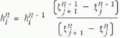
Here, sgn(u) = ±1, the sign depending upon whether u is positive or negative; ζ is the local inclination angle (Fig. 1); κ is the dimensionless curvature of the base; λ is the curvature-ordering parameter; e is the aspect ratio; κactpass is the earth-pressure coefficient, such that the normal stress components ρξξ and pηη are related by

where ϕ is the internal angle of friction.
This assumed constitutive behaviour is shown in terms of the standard Mohr diagram in Figure 2. We assume that an active or a passive state of stress is developed by noting whether an element of granular material is being elongated or compressed in the direction parallel to the bed. Thus,

Fig. 2. Mohr's circle in the coordinate system (normal stress, shear stress). Shown are internal angle of friction, ϕ, basal friction angle, δ, and two possible states of stress — active and passive.
normal and longitudinal stresses may be related through an earth-pressure coefficient, κactpass, defined by Equations (4) and (5).
Equation (2) is the integrated mass-balance equation, and has the familiar form of the kinematic wave equation. Equation (3) is the integrated longitudinal momentum equation. The first term on the right of the equation is the driving stress, which is due to gravity, and the second term is composed of two contributions, of which one is the ordinary Coulomb bed resistance and also arises on a flat bed, and the other quantifies the increase in bed pressure due to the centrifugal forces induced by bed curvature. Such centrifugal forces lead to a corresponding increase in drag force. The third term in Equation (3) is an averaged longitudinal stress gradient. For extensional flow, stress must occur in its active form; for contraction flow, a passive state of stress is established. Equation (2) is accurate to all orders of ε. Equation (3) is accurate to order ε (recall ε is the aspect ratio H/L) if tan δ ~ O(ε) and λ < O(1). These or stronger assumptions will be imposed in the sequel.
Boundary and initial conditions are

where R and F designate the rear and front ends of a pile. A detailed derivation of these equations is given by Savage and Hutter (in press), and a justification for the adequacy of the simple model represented in Equation (1) is given by Hutter and others in a forthcoming paper.
Procedure for obtaining numerical solutions
The governing depth-averaged Equations, (2) and (3), for the conservation of mass and momentum were solved numerically by means of a Lagrangian finite-difference method. Computation of the temporal development of an avalanche involves the determination of the position of the air-gravel interface, this giving a value for the depth of the granular material. A Lagrangian scheme is the natural choice for such a problem because it follows the motion of the deforming gravel mass.
We divide the granular mass of an avalanche into a number of cells, as shown in the depth profile of Figure 3. The mesh cell boundaries are advected with the particles. The cell boundary points are defined at times, t = n - 1, and are designated as (
where
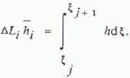

Fig. 3. The finite - difference net: granular pile is divided into cells whose boundaries are denoted j (j = 0,1, …, n). Velocities are made discrete both at cell boundaries and at he ights midway between these boundaries, point i being to the right of j.
Let us assume that we know ![]() and
and ![]() . At t = 0, we identify these with the initial values, and thus obtain the new positions for the cell boundaries,
. At t = 0, we identify these with the initial values, and thus obtain the new positions for the cell boundaries, ![]() , after a time interval Δt. Thus,
, after a time interval Δt. Thus,
We then determine the depth at the cell centres, i, using Equations (6) and (7), so that
Finally, we solve the depth-averaged momentum Equation (3), for the velocities at the cell boundaries

where
and
This numerical scheme is only conditionally stable. It is, however, a considerable improvement upon the other Eulerian scheme which we have already tried. For the calculation of points other than the leading and trailing edge end points we have added an artificial viscosity term, ![]() , to the right-hand side in Equation (II) and this will dampen the numerical ripples which some conditions have a tendency to generate. Values for the artificial viscosity, μ of between 0.01 and 0.03 proved to be adequate for our purposes, and using these values for μ is a standard procedure for manipulating parabolic equations involving advection and diffusion.
, to the right-hand side in Equation (II) and this will dampen the numerical ripples which some conditions have a tendency to generate. Values for the artificial viscosity, μ of between 0.01 and 0.03 proved to be adequate for our purposes, and using these values for μ is a standard procedure for manipulating parabolic equations involving advection and diffusion.
Computational Results
We now present a comparison between the experimental results for a selection of our experiments and the numerical predictions for these experiments, and then discuss some interesting features of the spreading of a pile of granular material along the curved bed of an avalanche path.
Inclined curved-chute experiments
The experiments were performed using a 100 mm wide chute which consisted of two straight sections, one inclined and the other horizontal, which had been connected by a curved, replaceable segment which allowed us to adjust the angle of inclination of the chute between 45° and 60°, as shown in Figure 4 (Reference PlüssPlüss, 1987; Reference Hutter, Plüss and MaenoHutter and others, 1988). A known mass of granular material was placed in the filling area at the upper end of the chute and was released by opening a shutter. The released material started to move, and while moving along the chute it was video-filmed and photographed. Usually six photographs were taken every second, and by proper setting of the time of initiation of motion, the photographs made possible our goal of determining the evolution of the geometry of the moving gravel mass through lime, with particular reference to its form and to its degree of extension into the run-out zone.
Two types of materials were used in our experiments. The first type was a collection of lens-shaped plastic

Fig. 4. Series of snapshots of a finite mass of 2000 g Vestolen particles moving down a chute. Inclined and horizontal parts are each 1.70 m long, radius of curvature of curved section is 0.245 m and generates an angle of inclination of α = 50°. Black lines on frontal Plexiglass wall mark increments of 50 mm, and long hand of the clock performs one revolution s−1 (experiment No. 88, Reference PlüssPlüss, 1987).
particles, Vestolen, with a mean diameter of 3.5 mm, bulk density of 540 kg m −3, and solid density of 950 kg m−3. The second type was composed of glass beads of 3 mm diameter, 1730 kg m−3 bulk density, and 2860 kg m−3 solid density. A detailed description of more than 20 of the experiments performed, and including a comparison of experimental results with those predicted from theory is given in Hutter and others (in press).
The pattern of evolution of the motion of an avalanche in one specific experiment is shown in Figure 5. For this experiment the inclined part of the chute was set at an angle of 50°. The distribution of the height of avalanche and, in particular, the front and rear ends of the avalanche body were photographed at a predetermined sequence of times. At t = 0, the avalanche front is observed to accelerate quickly whereas the rear end remains almost at rest for about half a second. The front travels a significant distance into the horizontal part of the chute before substantial deceleration is observed to set in. In contrast, the rear end comes quickly to rest once it has entered the horizontal part of the chute; the duration of the entire experiment is 1.4 s. Such data permit the determination of the development of avalanche spreading; for example, the positions of the leading and the trailing edges can be monitored over time, and the differences at various times will give the pattern of development of the length of the avalanche.
Comparison of Experimental Results With Computations
In an experiment prior to the release of granular material, the gate retaining the granules was positioned perpendicular to the bed of the chute channel. During the opening operation the material often remained in contact with the gate, so that formation of initial conditions were somewhat variable. We chose an initial profile that was close to the form of the mass at rest and avoided kinks and the generation of an overhang region. For our computations the parameters listed in Table I were selected. Comparison between experimental results and those predicted by computation are shown in Figure 5a-d. In these the changes in the positions of the leading and the trailing edges (Fig. 5a and c) and the corresponding changes in the simulated avalanche length (Fig. 5b and d) can be seen. At t = 0, the avalanche front accelerates quickly whereas the rear end remains nearly at rest for almost half a second. The front region travels a considerable distance into the horizontal part of the chute before substantial deceleration sets in; the rear end, however, comes quickly to rest once it has entered the horizontal part of the chute. Interestingly, the avalanche length goes through a maximum and then decreases again until it reaches its final value in the run-out zone.
Velocities of the avalanche front, dξf/dt, and rear,

Fig. 5. a, c. Front and rear end position (dimensionless coordinates) for experiments No. 87 and 28 plotted against dimensionless time. Circles show experimental results with error bars, solid lines are for computational results. b, d. Corresponding dimensionless avalanche length plotted against a scaled time for the same experiments.
Table 1. Conditions and characteristic constants for two experiments described in figure 5

dξr/dt, can also be calculated from our photographs, but in this case our deductions are less accurate, although agreement between experiment and theory is convincing to the same extent as that for the data used in Figure 5.
Similarity Solutions
For small bed friction angles and small values of the curvature parameter, it turns out that similarity solutions to the governing equations are possible (Reference Savage and NohguchiSavage and Nohguchi, 1988; Reference Savage and HutterSavage and Hutter, 1989; Hutter and Nohguchi, in press; Nohguchi and others, in press). In such cases the avalanche-depth profiles have the form of a parabolic cap and the difference velocity, obtained from the depth-averaged velocity minus the centre-of-mass of the moving pile varies linearly with distance from the centre of mass of the moving pile. The half-spread of the parabolic pile, g(t), the centre-of-mass position, ξ = x0, and the horizontal and vertical (downward) coordinates, X and Y,

Fig. 6. Definition sketch for construction of similarity solutions.
whose origin corresponds to the initial centre-of-mass of the pile at time, t = 0 (Fig. 6), obey the following six first-order ordinary differential equations:
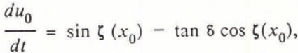

in which u0 is the longitudinal velocity of the centre-of-mass of the pile, and curvatures have been assumed to be small (Reference Savage and NohguchiSavage and Nohguchi, 1988).
The six differential Equations (14)-(19) were integrated in a straightforward manner using a fourth-order Runge-Kutta technique. It is found that:
For cases in which the bed inclination angle monotonically decreases with distance down-stream, the pile of granular material starts from rest, initially accelerates, and then decelerates, finally coming to rest as a result of bed friction and of the gradually decreasing bed slope. It is found that the variation of the total length with time can exhibit differing patterns, depending upon frictional parameters, the shape of the bed, and the initial depth to length ratio of the pile. Amongst the possibilities are that the pile can grow monotonically, that it can asymptote to a constant length, that it can grow to a maximum and then decrease, or that it can decrease to a minimum and thereafter increase with time. Furthermore, there are regions in parameter space for which the pile moves as a rigid body either for the whole time of travel or for parts of it. Figure 7 shows some typical results for the half-spread of the pile, g(t), plotted against the centre-of-mass position, ξ = x0, and time, t, for a bed having the form of a circular are. The bed inclination angle is given by ξ = ξ0(1 - aξ), where ξ0 is the initial bed slope, and a is a constant. Results shown in the figure are for various initial values of ε, and for θ0 = 40°, a = 0.1, a bed friction angle, δ = 10°, and an internal friction angle, ξ = 25°.

Fig. 7. Evolution behaviour of g(t) for a circular arc bed profile; ξ0 = 40°, a = 0.1, δ = 10°, ϕ = 25°. Effect of varying initial depth to length ratio, ε, is shown. Rigid regions are cross-hatched.
Variation in Basal Friction
The above results were obtained by application of the simple Coulomb-type sliding law. Several more realistic forms can be introduced and surprising results sometimes emerge when this is done. We are presently studying various extensions (Hutter and Nohguchi, in press; Nohguchi and others, in press); here some of the results are briefly discussed.
Consider the case that the friction angle, tan δ = μ, varies along the avalanche bed, is largest at the front, and is smallest at the rear end. For a linear variation of μ, such a dependence may be expressed as

where the subscripts, F and R, refer to the front and rear ends of the avalanche, respectively. Such a basal friction law accounts for the fact that an avalanche may deposit snow along its track and thus smooth it. Alternatively, the law expressed in Equation (20) may be interpreted to make it possible to account for some of the observed ploughing effects.
We have already analysed equations corresponding to Equations (14)-(19) in an earlier paper (Nohguchi and others, in press), with the sliding law, Equation (20), incorporated. Here we discuss results for the case of a planar surface. Figure 8 displays phase space orbits g against ![]() in panel (a) for δ = constant, and in panel (b), when Equation (20) was used. To obtain these plots, we integrate Equations (14)-(19) for specified initial conditions, g(0) = g0,
in panel (a) for δ = constant, and in panel (b), when Equation (20) was used. To obtain these plots, we integrate Equations (14)-(19) for specified initial conditions, g(0) = g0, ![]() , and thus compute g(t) and
, and thus compute g(t) and ![]() . For each initial condition a particular curve in phase space is obtained. Data chosen for our treatment are as follows:
. For each initial condition a particular curve in phase space is obtained. Data chosen for our treatment are as follows:  .
.
To interpret the plots which are presented, consider a granular avalanche starting from rest, that is at point C in Figure 8a. As the avalanche moves down the chute the corresponding point in phase space moves along an orbit to the right (point D). It can be seen that the granular pile is always monotonically extending for all choices of points C, so that g is growing to the right.
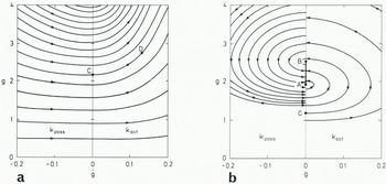
Fig. 8. Phase space orbits g against ![]() for an avalanche sliding down an inclined plane: (a) with constant basal friction, (b) with variable friction according to Equation (20). C represents the avalanche at rest, D are points generated when it is moving. AB represents the segment of states for rigid-body motion.
for an avalanche sliding down an inclined plane: (a) with constant basal friction, (b) with variable friction according to Equation (20). C represents the avalanche at rest, D are points generated when it is moving. AB represents the segment of states for rigid-body motion.
In Figure 8b the qualitative behaviour represented is quite different. If the starting point C is below A, then the avalanche will be extending with time, until its orbit in phase space again coincides with the g-axis. If this point of the orbital trajectory is above point B in Figure 8b, then the motion will continue along the trajectory to the left, with ![]() ; thus g will now decrease until the position of the axis
; thus g will now decrease until the position of the axis ![]() is again reached. If the intersection between the orbital trajectory and the axis
is again reached. If the intersection between the orbital trajectory and the axis ![]() lies between A and B, then the avalanche length remains constant for all time, that is
lies between A and B, then the avalanche length remains constant for all time, that is ![]() . This can be shown by a careful analysis of Equations (14)-(19), and it is seen that for all initial conditions for the choice of point C on the axis g = 0 the trajectory of the motion will eventually lie between A and B.
. This can be shown by a careful analysis of Equations (14)-(19), and it is seen that for all initial conditions for the choice of point C on the axis g = 0 the trajectory of the motion will eventually lie between A and B.
The physical interpretation of the nature of the segment AB is important in this description; it represents all those states, ![]() , for which the avalanche moves as a rigid body. The existence of this rigid-body state for the motion along an inclined plane is due both to the variability of the basal friction coefficient and to the fact that κact/κpass ≠ 1. As κact becomes closer to κpass the points A and B will coalesce, but as μF tends towardsμR the distance AB will move to infinity along the g-axis. In this latter case the situation shown in Figure 8a is re-established.
, for which the avalanche moves as a rigid body. The existence of this rigid-body state for the motion along an inclined plane is due both to the variability of the basal friction coefficient and to the fact that κact/κpass ≠ 1. As κact becomes closer to κpass the points A and B will coalesce, but as μF tends towardsμR the distance AB will move to infinity along the g-axis. In this latter case the situation shown in Figure 8a is re-established.
In closing, we should mention that even though the motion of a granular pile along an inclined plane terminates as a rigid-body motion the centre of mass motion of the pile is still accelerating. Hutter and Nohguchi (in press) show that in order for a granular pile to be able to reach both a rigid-body state and a finite steady velocity, a viscous sliding term of the form shown in Equation (1) must be included in the theoretical model.
Concluding Remarks
The present paper has made use of the depth-averaged equations of motion of Reference Savage and HutterSavage and Hutter (1989, in press) and has obtained numerical solutions to describe the motion of a finite mass of gravel down an inclined chute. In view of the simplicity of the physical model, which treated the granular material as an incompressible continuum with uniform density and applied depth-averaging to the velocity field, the correlation between predictions and the laboratory experiments is surprisingly good. Incorporation of more complex basal friction laws has demonstrated that a significant influence on the gravel motion is exerted by specific resistance properties of the basal surface. Many more experimental results have been obtained, and will be reported by Hutter and others (in press). Further analytical work is in hand, in which effects of density changes as a result of fluidization, and higher-order effects of bed curvature are considered, as well as possible extensions to the three-dimensional processes to be incorporated (Reference Lang, Leo and HutterLang and others, 1989).
Acknowledgements
We thank D. McClung and H. Norem for their careful review of an earlier draft.


