


Introduction
Accurate maps of glaciers are essential for water resource management and hydropower planning in many mountainous areas. Repeated mapping is needed to keep track of changes of glacier volume in response to mass-balance variations. An early signal of changes of volume in response to climatic variations is likely to be provided by changes of the amount of annual accumulation and ablation, with their consequent effect on surface elevation. However, the poor weather conditions, including frequent cloud cover, to which glaciers, and particularly their accumulation areas, are prone hinder repeated mapping by conventional aerial and terrestrial surveying techniques. Recent developments of global positioning systems (GPS) have provided opportunities for rapid and frequent mapping, overcoming many of the problems experienced during conventional surveys. High-precision data relating to glacier surface topography can be obtained rapidly and very efficiently by using a GPS in kinematic mode (Hulbe and Whillans, 1994a, b).
In July 1995, three-dimensional positions of more than 2200 points were acquired during a differential kinematic GPS survey of the accumulation area of Austre Okstindbreen, the largest glacier of the Okstindan area, Norway (66°00' N, 14°10' E). The survey, completed in less than 6.5 h, was undertaken with a roving geodetic-quality GPS receiver mounted on a snow scooter, whilst a similar reference receiver recorded data at a fixed station. Dual frequency observations, using both code and phase (L1 and L2) carriers, were made and post-processing of the data was undertaken using Leica’s SKI software. A detailed triangular irregular network digital terrain model (TIN DTM) of the accumulation area was constructed from the data. Because the three-dimensional positions of the apices of each triangle were defined precisely by the differential-mode GPS survey, they provided substantial detail about the variations of aspect and gradient of the snow-covered surface.
Study Area
Austre Okstindbreen is the largest glacier of the Okstindan area, with a surface area of about 14 km2, of which about 12 km2 is above the mean equilibrium-line altitude (ELA) of recent years (1250 m). The highest parts of the accumulation area, on the slopes of Oksskolten, northern Norway’s highest mountain, are more than 1650 m a.s.l. An icefall, which descends from about 1250 m to 1000 m, separates the upper and lower parts of the glacier. The terminus is at 733 m.
General circulation models suggest that the Okstindan area, which is close to the latitude of the Arctic Circle, may experience particularly intense warming in the future, associated with changing atmospheric composition (Hansen and others, 1988). Austre Okstindbreen is included in the Norwegian national network of glacier mass-balance observations. Whilst its terminus has experienced annual net retreat throughout the last 25 years, its net mass balance has been positive in six of the nine mass-balance years since 1986–87.
Terrestrial photogrammetric surveys of the lower part of the glacier were undertaken in most summers between 1978 and 1991, as part of the programme of the Okstindan Glacier Project. The surveys did not extend to the accumulation area, but observations have been made there since the start of the project. Aerial photographs taken in September 1981 provided the basis for a 1:10 000 scale map of the whole glacier.
Surveys Of The Accumulation Area, 1981 And 1993
The aerial photographs of Okstindan taken in 1981 were used by the Norwegian Mapping Authority (Statens kartverk) to produce maps (contour interval 20 m) which include Austre Okstindbreen. Minor inaccuracies in some of the accumulation area contours have been identified. These reflect the difficulties encountered in stereoscopic viewing and photogrammetric contouring of snow-covered areas where shadows, structural features, debris and dust are absent from the surface (Østrem, 1966).
In 1993, three-dimensional positions of 253 points in the accumulation area were determined by electronic distance measurements; a total of more than 30 h was required to complete the EDM surveys, because of poor weather. The number of positions included in the survey was limited by the time taken in moving the reflecting prisms from one point to the next. The 1993 data were incorporated into a geographic information system (GIS), and a TIN DTM of the accumulation area surface was constructed (Theakstone and Jacobsen, 1995).
Gps Surveying At Austre Okstindbreen
Background
GPS surveys ran be carried out in weather conditions which prohibit both photogrammetric and EDM surveying and can In- undertaken by one person. Differential GPS surveys make use of two receivers, one of which (the reference receiver is stationary, whilst the mobile receiver is moved to a succession of survey positions. Information transmitted by the constellation of 34 Navstar satellites is used to determine the positions of the receivers. The receivers record simultaneously the distances (ranges) between them and the satellites. Ranges to three satellites provide a good spatial fix of the position of the receiver if the satellites are well distributed. Poor spatial configuration of the satellites, which is expressed by the geometric dilution of precision (GDOP) recorded by the GPS receivers, results in ambiguities. These can be resolved by a fourth range measurement. By measuring the arrival times of signals from four satellites, the receiver can compute a four-dimensional space–time fix in the WGS-84 geodetic reference system. Signals from the satellites are transmitted on two radio frequency carriers, in code (L1) and in phase (L2); measurement of phase of the incoming GPS carrier ensures high precision. Differential post-processing of the data acquired simultaneously by the two receivers permits corrections to be made for variations in transmitted signals and in the ionosphere and atmosphere. The processing removes errors and permits the ranges to he determined with a high degree of accuracy. In order to transform the GPS solution based on the WGS-84 datum into the local grid coordinates, transformation parameters based on the coordinates of several points in both geodetic data have to be determined.
The 1995 survey
In 1995, the positions of the reference station (base hut) and stations An and As (Fig. 1) were determined, using a static GPS survey. Stations An and As had been occupied during surveys of accumulation area (mass-balance) stake and pit positions in previous years. Three trigonometric stations,
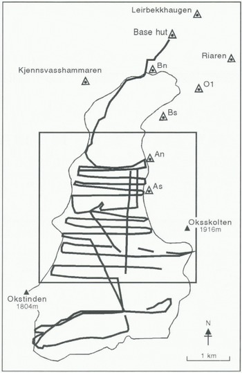
Fig. 1. Stations occupied during static GPS surveys at Austre Okstindbreen (triangles) and the tracks used in kinematic surveys (solid lines). The glacier margin is plotted from digital data, based on aerial photographs taken in 1981. supplied by the Norwegian Mapping Authority. The box indicates the area shown in Figures2–5.
Riaren, Leirbekkhaugen and Kjennsvasshammaren (Fig. 1) were occupied by a roving GPS receiver in the course of the 1995 survey. As a result of this survey, all previously recorded coordinate data from the accumulation area of Austre Okstindbreen have been related to the national grid, UTM zone 33.
The reference receiver was mounted on one corner of the base hut roof, at 850 m a.s.l., for some of the kinematic GPS surveys. For others, in order to keep the separation of the reference and roving receivers below 10 km, it was sited at higher altitudes. There was no physical connection between the reference and roving receivers, which generally were not within line of sight of each other. All surveys were undertaken when at least four Navstar satellites were known to be visible. Lock was maintained on six to eight satellites for most of the time, with a GDOP value of 4 or less, so that ambiguities were resolved without difficulty.
When GPS surveys were conducted in kinematic mode, the roving receiver was mounted on a snow scooter, with the antenna at a fixed height (1.48 m) above the surface, sufficient to leave the antenna clear of interference. For most kinematic surveys, a near-constant speed of 20 km h−1 (5.6 m s−1) was maintained. With a recording rate of 10 s, the along-track separation of recorded points was approximately 56 m. Where surface topography was less varied, the speed at which the snow scooter was driven was increased to 30 km h−1, giving an along-track separation of approximately 83 m. Pauses were made at a number of points, including stakes used in mass-balance observations; collecting two epochs of data (20 s) was sufficient to fix their positions.
Three-dimensional positions of 2228 points, most of them on transverse profiles across the glacier’s accumulation area (Fig. 1), were obtained in less than 6.5 h by the scooter-based kinematic GPS surveys. Time constraints prevented the survey of one planned traverse, about 1 km north of the glacier’s southern border. The precision of the three-dimensional coordinates in theWGS-84 system was 0.01–0.02 m. Error calculations are based on the variance–covariance matrix of the averaged multiple position determinations from the GPS. An error ellipse, which represents a two-dimensional (horizontal coordinates), 1 s level confidence region, is computed. There is a 39% probability that the determined point lies within this error ellipse. The vertical accuracy is computed as a one-dimensional, 1 s level confidence region; there is a 68% level of confidence that the height is within the specified region. Normally, the SKI post-processing software automatically removes any point that does not satisfy the ±0.02 m criterion for both horizontal and vertical error. However, automatic selection was overridden in plotting the 1995 GPS data, and a detection criterion of 0.10 m was used.
As the precision of the Norwegian control points in the area is not known, the positions were transformed to UTM coordinates using an interpolation technique. The differences of the six distances between four control points, Riaren, Leirbekkhaugen, Bn and Bs (Fig. 1), computed in both UTM and WGS-84 coordinates, ranged from -0.03 to +0.06 m. For purposes of comparison, a classical seven-parameter transformation, which preserved the geometry of both the WGS-84 and UTM networks, was applied to the data, using two points, Riaren and Leirbekkhaugen (Fig, 1). The computed residuals in geodetic coordinates were: latitude 0.139 m; longitude 0.0326 m; height 0.0736 m.
Digital Terrain Modelling Of The Accumulation Area
Three TIN DTMs of the accumulation area of Austre Okstindbreen have been constructed. Digital (contour) data from the 1981 aerial photogrammetric mapping, provided by the Norwegian Mapping Authority, were used to construct one model. A second was constructed from the 1993 EDM data and a third was based on the 1995 GPS survey. The original, irregularly spaced data points were used in constructing the models.
The surface within a TIN UTM consists of facets, each of which is defined by three precise three-dimensional coordinates. Because the modelled surface passes through all the original data points, no interpolation is necessary. This is a major advantage over regular grid-based DTMs, but interpolation is necessary with both types of model if contours are to be constructed. In the 1981 model, the previously defined contours were used as fixed data (elevation) points. In the digitising process, each contour was followed and xy coordinates were determined at closely spaced intervals; these
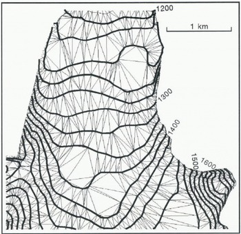
Fig. 2. A triangular irregular network (TIM) model of the northern part of the accumulation area of Austre Okstindbreen. Contours (20 m interval) drawn from a 1981 aerial photogrammetric survey were digitised to provide the basis for the terrain model. The apices of each facet lie on the contour lines. The facets are larger where the surface gradient is lower and the topography is relatively simple.
then were thinned, by reducing the number of points in areas where the contour was rather uniform, and leaving a larger number of points where the contours were more irregular. Thus, the digital data have a fixed elevation, whilst the spacing of the xy points varies. In the 1981 TIN model, therefore, most facets are defined by two xy coordinates on one contour, and one xy coordinate on an adjacent contour, whilst a few have all three apices at the same elevation. The
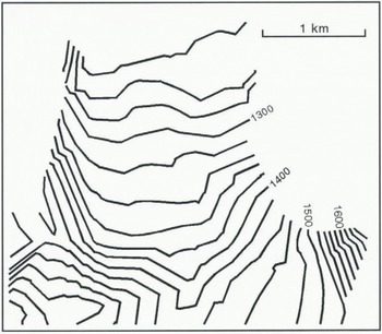
Fig. 3. A contour map based on the 1993 TIN model of the northern part of the accumulation area of Austre Okstindbreen. The model was constructed from data obtained by electronic distance measurements to 253 points. The angularity of the contours reflects the spatial distribution of these points and the contouring method.
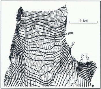
Fig. 4. Part of a TIN model of the accumulation area of Austre Okstindbreen based on differential kinematic GPS surveying in 1995. The angularity of the contours on the sleep slopes below Oksskolten (bottom right) results from the sparsity of surveyed points in that area.
facets preserve the pattern of wider spacing (larger triangles) in areas where the surface topography is relatively simple, and smaller triangles where it is more varied (Fig. 2).
The triangular facets in the 1993 TIN model are defined by the three-dimensional coordinates of the 253 points which were surveyed by EDM: the apices of every plane triangular facet are points included in the survey. Several of the facets are very large, because of the relatively small number of points fixed by the survey, and some of these large facets are directly adjacent to much smaller ones which represent areas where the surface is better defined. Contours (10 m interval) were constructed by intersecting the facets by planes at fixed elevations. The contours therefore are straight-line segments across the facets. As a result of the spatial distribution of the original data points, some of the contours are very angular (Fig. 3). The presence of such artefacts of the contouring process in some areas limits the opportunities for direct comparison of 1993 elevation data with models from other years.
The mean concentration of the data acquired in 1995 is about 182 points km−1, so the TIN DTM of the accumulation area of Austre Okstindbreen (Fig. 4) is more detailed than those of 1981 and 1993. Most of the triangular facets have areas of less than 9000 m2. The high density of the surveyed points provided an excellent basis for interpolating contours. However, the wider spacing of the surveyed points in some areas results in angularity or incorrect placing of the contours there: the method of surveying, whereby most points are closely spaced (50 m) on cross-profiles which are significantly further apart (200 m on average), can create contours which appear artificial, because they are formed by linear interpolation, and consist of straight-lines segments across the individual facets.
Changes Of The Accumulation Area, 1981–95
The 1981 and 1995 TIN DTMs have been used to investigate changes of surface elevation and topography of the lower part of the Austre Okstindbreen accumulation area during the last 14 years (Fig. 5). Changes of the area’s boundaries in recent years have been slight, and the same irregularly spaced data points therefore were used to define matching boundaries for the two models. The accuracy of contouring snow-covered surfaces by aerial photogrammetry using a camera of a particular focal length depends on the flying height and the surface slope (Blachut and Müller, 1966). The probable errors in position and height of the contours based on the 1981 aerial photogrammetry of Austre Okstindbreen are of the order of 5 and 0.3 m for 2° slopes, respectively; for slopes of 15°, they are 1.5 and 0.6 m, The accuracy of the 1995 GPS data, noted above, was an order of magnitude better than that of the 1981 aerial photogrammetric data, and the linear interpretation technique used in constructing the 1995 contours from the TIN model introduced no errors greater than those of the 1981 contours. Elevation changes were calculated by projecting the xy coordinates of the 1981 TIN DTM onto the 1995 surface, The maximum error of the calculated change of elevation at any point in the xy plane is considered to be 1 m, and all changes greater than that are real increases or decreases.
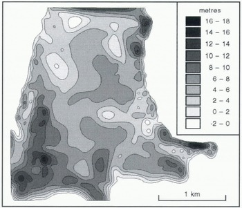
Fig. 5. Changes of surface elevation of part of the accumulation area of Austre Okstindbreen, 1981–95.
Most of the snow which accumulates on the glacier is associated with air masses which arrive from the southwest or west, and net accumulation is high in the lee of the mountain Okstindan. A ridge of elevated surface topography extends from the northeast ridge of Okstindan, and it is this area which experienced the greatest change of surface elevation between 1981 and 1995. The comparison of the two TIN DTMs indicates that, in the 14 year period, the glacier thickened by up to 18 m in the southwestern part of the sample area, whilst thinning of the lower part of the accumulation area, around the mean ELA of recent years, occurred, notably in the northwest (Fig. 5).
Aspect And Gradient
Handling the substantial body of three-dimensional digital data acquired during a GPS survey within a GIS permits the creation of new topographical indices. Combinations of surface aspect and gradient, which are important in relation to energy inputs and to the glacier’s response to mass-balance perturbations, have been defined for the lower part of the accumulation area of Austre Okstindbreen, using the 1995 TIN DTM. The original facets were combined to produce a smaller number of larger areas, for each of which the orientation and slope were calculated (Fig. 6). Such a combination of aspect and gradient can be used to produce data about spatial variations of radiation input, thereby improving energy-balance calculations, especially when the shadowing effects of adjacent mountainous terrain are included in the models.
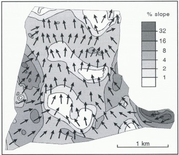
Fig. 6. 6Gradient and aspect at the surface of the accumulation area of Austre Okstindbreen are combined in this map, using 1995 GPS data. Arrows indicate the orientation of the maximum slope within irregular triangular facets.
Discussion
Most of the errors in GPS data collection are removed by differential techniques in post-processing, because the reference receiver computes errors associated with the satellites, and the corrections are applied to the data from the roving receiver. Only those sources of error which are not common to both receivers are not removed during differential correction. The most likely such source at Okstindan is a surface-reflected signal which reaches the receiver at the same time as a direct one. The probability of such multipath errors arising is reduced by avoiding the use of signals from satellites at low elevation above the horizon. The directional-type antennae used during the GPS surveys at Austre Okstindbreen are designed to reject multipath errors. Furthermore, the satellite-trajectory masking angle was set at 15° for the 1995 survey, and a minimum acceptable signal strength was set, so that signals more than 40 dB weaker than the strongest signal received by the receiver were rejected. GPS errors therefore presented no significant problems.
Repeated GPS surveys can detect seasonal, annual and longer-term changes of glacier thickness and are likely to provide a rapid and precise means of determining glacier mass balance (Hulbe and Whillans, 1994b). This is of particular value in the accumulation zones of glaciers. Hulbe and Whillans (1994b) reported that post-processing of data acquired during a “stop-and-go” survey with a geodetic-quality GPS receiver placed on the tops of marker poles near the South Pole and a stationary receiver at the Pole produced relative positions accurate to 0.01 m, and that similar kinematic GPS surveys elsewhere in Antarctica yielded accuracies of 0.005 m km−1. Hulbe and Whillans (1994a) surveyed the positions of about 270 stations on Ice Stream B, Antarctica, in two successive summers, using a “stop-and-go” GPS technique. The horizontal precision was similar to that of traditional surveying methods, but the vertical precision was much better and permitted the daily variability of snow elevation caused by firn settling and wind action to be determined. Root-mean-square differences of horizontal and vertical components of position of the Ice Stream B stations were 2.5 and 5.5 mm km−1, respectively, when post-processing software was used, and 1.5 and 5 mm km−1, respectively, when an algorithm which identified vectors which did not conform with repeat and neighbouring observations was applied to the data. The acquired data provided the basis for determination of horizontal velocity gradients and strain rates, for calculations of the vertical velocity of each of the surveyed poles relative to that of a reference pole and for a contour map (2 m interval) of the 170 km2 area. These relative vertical velocities were accurate to 20 mm km−1 a−1. Vaughan (1994) concluded that the limit of uncertainty of the kinematic GPS method which he used to locate the limit of tidal flexure on Rutford Ice Stream, Antarctica, was around ± 3 cm, whilst the method of mounting the receiver on a Skidoo and driving introduced a further ± 8 cm. During the kinematic GPS survey at Austre Okstindbreen, tests indicated that the inaccuracy caused by mounting the receiver on the snow scooter was ± 6 cm on level ground. Tilting on steeper slopes did not increase the uncertainty by more than 2 cm. Overall, the heights of points determined by the 1995 differential GPS survey are believed to be accurate to ± 0.10 m, and the changes of elevation between 1991 and 1995 determined by comparison of the results of the aerial photogrammetric survey in the earlier year and the GPS survey are considered to be within 1 m of the true values.
Conclusion
Glacier mass-balance studies are likely to be improved significantly by means of kinematic GPS surveying, with which data relating to a very large number of points at the surface of a glacier can be acquired in a short time, and which can be carried out in weather conditions that prevent optical surveying. Accurate three-dimensional positions of more than 2200 points on the featureless snow-covered accumulation areas of Austre Okstindbreen were obtained in 6.5 h of kinematic differential GPS surveying in 1995. The speed and accuracy of the technique make it particularly suitable for repeated glacier mapping, especially by surveys of glacier surface profiles. Repeated GPS surveys will have great utility for early detection of the effects of climate change, especially the first detection of changes of glacier thickness. Incorporating the results of the surveys in a GIS facilitates the construction of DTMs of the glacier surface and permits the construction of detailed maps and further models in which elements of the surface topography, such as aspect and gradient, can he combined. Such detailed maps of glacier surface form have considerable potential utility in energy-balance investigations.
Acknowledgements
The studies reported here were undertaken during the tenure of a research gram (GR3/8373) from the U.K. Natural Environment Research Council (NERC). The snow scooter used during the survey was purchased with the aid of a previous NERC research grant (GR3/7253). The Okstindan Glacier Project is supported by Statkraft, the Norwegian Power Authority. We are pleased to acknowledge financial support from the University of Manchester, the Leverhulme Trust and the British Council. We are grateful to other members of the Okstindan Glacier Project, especially N.T. Knudsen and P. Raben, for assistance in the field, and J. T. Møller, for terrestrial photogrammetric mapping. We are indebted to B. Whalley of The Queen’s University, Belfast, for making the GPS equipment available to us, and to S. Mears of Leica UK. Limited for advice.


