


1. Introduction
The wide range of mathematical models which has been developed for hydrological forecasting and planning reflects the considerable variation in scale (1 to 105 m) at which hydrological processes are considered. At one end of tne range, for example, a realtime flood forecasting model may treat a river basin of, say, 100 km2 as one unit (a “black-box”) and relates rainfall input over the whole basin to river flow output. On the other hand, hydraulic models used to design river engineering works may describe the flow of water within the river channel on the 1 to 10 m scale.
On the large scale, the model equations are likely to be derived from systems theory and the parameters reflect the nature of the system (size, geomorphology, etc.) as well as the hydrological processes. Thus it is difficult to estimate parameter values for one system from those known for another. For such models parameter values have to be determined from historical cal records of outputs of the system to be modelled minimizing the difference between predicted and measured data. On the small scale, the model equations are based on the physics of the hydrological processes and the parameters are far less dependent on the nature of the system. Thus they may more easily be specified a priori for a given application. For example, the values of hydraulic conductivity required in a physics-based infiltration model for a field plot may be specified on the basis of results from laboratory experiments.
When output data are available for optimization of the parameters the large-scale or “lumped” hydro-logical models are effective and simple to use. However, when such data are not available, for example if the effect of possible future changes to a system is to be investigated, the small-scale, physics-based “distributed” models have the advantage.
Physics-based equations have been developed for most hydrological processes and tested by laboratory and small-scale field experiments. These established equations are now being combined to create distributed models of the entire land phase of the hydro-logical cycle. In particular, the Système Hydrologique Européen (SHE) has been developed jointly by the Institute of Hydrology (UK), Sogréah (France), and the Danish Hydraulic Institute.
This paper describes a distributed model of snow-melt which has been developed for use in SHE. There is a strong argument for matching the levels of analysis used for each hydrological process in a general model. For this reason the complexity of the SHE snow-melt model has been influenced by the state of the art in modelling other processes. For example, évapotranspiration is calculated using equations for the transfer of energy from the atmosphere to the vegetation which require full meteorological input data. Energy transferred to the snowpack is therefore calculated using the same “energy-budget” equations rather than the simple temperature-index method. Again, flow within the soil is modelled using Richard’s equation for flow in porous media and therefore the same equation is used to model flow within the snow. In one respect the snow-melt model is more complex than the rest of SHE. Since snow-melt is so critically dependent on heat transfer, the flow of energy as well as of mass and momentum has been modelled.
In the next section the equations of the SHE snow-melt model are derived. The theoretical background is given in some detail so that the various approximations made in this model may be compared and contrasted with those used in other physics-based, distributed models of snowpack behaviour.
2. Theory
The equations required to describe the flow of mass and energy in snow are the equations of conservation of mass, momentum and energy and an equation or equations of state. The snow is treated as a mixture of the three phases of water and air and each element of volume dV is assumed to contain many grains of ice dispersed within it. The subscripts i, w, v, a are used to denote ice, water, water vapour and dry air, respectively. When the two gaseous components are taken together subscript g is used.
2(a). Conservation of mass
The continuity equation for component k in one dimension is
where ρk is the density of component k, θk the volume per unit volume of snow, νk the velocity and Skj is the mass of component k produced per unit time per unit volume of snow by a phase change from component j. By definition, S kj = −S jk and S aj = θ. The water vapour and air occupy the same volume so θa = θν = θg and θi, + θW + θg = 1.
2(b) Conservation of momentum
be the density, pressure and momentum of the mixture. The velocity of its centre of gravity is ν. Then

where g is the acceleration due to gravity and T ZZ is normal stress in the z direction. In the SHE models of water flow in rock and soil this equation is replaced by the empirical Darcy law for flow in porous media. Hence this approximation is also made in the snow-melt model. Male and others (1973) discuss the conditions under which this approximation is valid. Separate equations may be written for water and moist air. Thus
where Kk is the hydraulic conductivity of the ice matrix for component k. The velocity of the centre of gravity of the moist air is
and the velocity of the water vapour with respect to this is
(Reference SulakvelidzeSulakvelidze 1959). 0 is the diffusion coefficient of water vapour in air.
2(c) Conservation of energy
The first law of thermodynamics may he written in terms of the enthalpy H, heat flow Q, and volume V, as
The change in enthalpy is
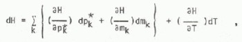
where pk = θkpk and mk = ρk θkV, The partial specific enthalpies are related to the latent heats by equations

where Ljk the latent heat produced by transformation of unit mass of component k to component j. Since
the increase in enthalpy from phase change per unit time may be written
If the specific heat at constant pressure of component k is (Cρ)k the change in enthalpy with temperature per unit time may be written
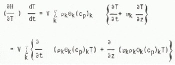
by the continuity Equation (1). The heat flow term may be expanded as
where k is the thermal conductivity of the mixture and SR are sources (6) may be written of radiant energy. Thus Equation (6) may be written
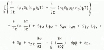
The last three terms are treated as negligible. Male and others (1973) discuss them in detail.
2(d) The equations of state
The equations of state of a snow sample are relations between values of the thermodynamic variables throughout the history of the sample. For modelling purposes it is useful to try to derive equivalent equations in terms of the present values. To do this it is necessary to specify the detailed distribution of each component of the mixture (which is the result of the sample history) and the detailed thermodynamic processes taking place within the mixture.
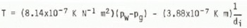
The ideal gas equation of state may be applied to the air and water vapour to give
where Mk is the molecular weight of component k and R is the gas constant. Reference YenYen (1962) has suggested that Pv should be set equal to the saturated vapour pressure for snow ps, which is known as a function of T. The empirical “characteristic” equation for snow may also be used as an equation of state. In a form commonly used in soil physics
where Ψa is the air-entry potential and α is an index of pore-size distribution. The set of equations must be completed by some relation between T and θw (or pw). Most previous authors (e.g. Reference YenYen 1962, Col beck 1972, Obi ed and Rosse 1977) have chosen the simplified relations
where T0 is the melting point at STP. Thus the snow is allowed to exist in two states, cold and dry, or ripe, and there is an abrupt transition between the two. This is not a very satisfactory solution for a general model especially since the discontinuity can provoke instability in finite-difference versions of the model equations.
An alternative approach is to postulate that the Gibbs function of the mixture is at a minimum for a given bulk temperature and pressure:
For certain simple configurations of the mixture the Gibbs function can be specified so an equation of state may be derived. Colbeck (1975) considers a mixture of spherical ice grains of constant diameter di, water and moist air. In the “funicular” regime the water content is high and the gas bubbles, assumed to be of diameter dg do not touch the ice. In this case Equation (17) leads to a simple expression for the temperature of the mixture in terms of its structure, namely
In the “pendular regime” of low water content, where there are interfaces between all three components of the mixture, Colbeck originally derived the equation
from Equation (17). However, he pointed out later (Colbeck 1979) that in the pendular regime a system of spherical ice grains of constant diameter cannot be in mechanical equilibrium. Equilibrium is possible if the ice grains are gathered in clusters of “compressed” spheres. If di/2 is defined as the radius of the ice-gas interface, Equation (19) holds, but there is a restriction on the configuration of the cluster imposed by the requirement for mechanical equilibrium. Colbeck suggests that the rate at which the cluster configuration can change limits the rate at which the mixture can proceed from one thermodynamic state to another and may even prevent states of high negative pw being reached. However, his analysis concerns an isothermal, homogeneous mixture in which the only process which can change the cluster configuration is slow mass diffusion in the immediate locality of the cluster. For a non-homogeneous snow cover with connective transfer of mass and latent heat flow the required metamorphism may be far less restrictive.
2(e) The single-phase flow approximation
This approximation is used in the SHE soil and groundwater flow models and hence also in the snow-melt model. It is assumed that the ice matrix is at rest, i.e. νi = 0 and that the moist air pressure is constant, i.e. pg = po. A-new variable, the capillary tension is defined: Ψ = pw - pg. The model equations are written in terms of the water phase only and consist of Equation (1) and Equation (3) (with k = w and |S wi| assumed much larger than |S wv|, Equation (15) and equations based on (13) and (19). The new energy equation is written
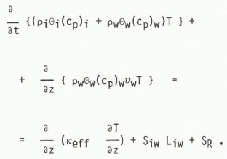
The heat capacity of the gaseous phase, has been neglected and the convection term for the moist air and two of the latent heat-source terms do not appear. Instead, an effective thermal conductivity Keff is defined which allows the effects of transport of vapour to be taken into account indirectly. Since there is only one explicit ice-source term
Equation (19) is used in the pendular regime and the expression
is used for saturated snow. In the transitional region between the pendular and saturated regimes the expression
is used, with coefficients chosen so that values of T and ?T/?Ψ are matched at the boundaries.
One last equation is needed to complete the model. This should relate changes in phase to changes in the distribution of the ice-water-vapour mixture. Equations (19), (22) and (23) are derived on the assumption that all the ice grains are of the same size. This implies that the phase changes have an equal effect on all grains in a given volume element. Hence,
and the number of grains is conserved. This is obviously an extreme simplification of snow metamorphism.
3. Values for the Model Parameters
3(a) Effective thermal conductivity
Equations (20) and (16) may be combined to give an equation for heat flow in cold dry snow:
which has been used to determine the effective thermal conductivity ![]() from laboratory experiments. This conductivity is not quite the same as K
eff. since a different equation of state has been assumed, but will be a reasonable approximation. Reference MellorMellor (1977) has summarized the data available on the variation of
from laboratory experiments. This conductivity is not quite the same as K
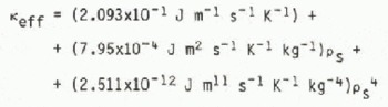
eff. since a different equation of state has been assumed, but will be a reasonable approximation. Reference MellorMellor (1977) has summarized the data available on the variation of ![]() with density. At a given value of ρs = ρiθi experimental values can vary by a factor of two, so an empirical equation for k
eff can only be approximate. The equation used in the SHE model is
with density. At a given value of ρs = ρiθi experimental values can vary by a factor of two, so an empirical equation for k
eff can only be approximate. The equation used in the SHE model is
3(b) Characteristic equation parameters
There are few data reported in the literature on the variation of water content with capillary pressure in snow. Col beck (1975) reports measurements made in an adiabatic environment on snow of density 550 and 590 kg m−3. Reference WankiewiczWankiewicz (1978) has made similar measurements on two samples of snow of density 360 kg m−3. De Reference QuervainQuervain (1973) gives water contents in two zones, a capillary zone for which Ψ can be specified and an equilibrium-free drainage zone where Ψ is not known but is probably more negative than 100 N m−2. De Quervain’s results are consistent with those of Col beck and Wankiewicz.
These data have been used to estimate Ψa and α in Equation (15). There are not enough data points for any particular variation with density or grain size to be deduced. The best straight line through all the data has a = -0.93 ± 0.12 and ln(-Ψa /N m−2) = 5.3 ± 1.5 which is equivalent to Ψa = -206 N m−2 (+161 or -692 N m−2 ). Reference WankiewiczWankiewicz (1978) gives wetting values of Ψa = -230 N m−2, -440 N m−2 and drying values Ψa, = 320 N m−2, -640 N m−2 for two samples.
3(c) Hydraulic conductivity
The hydraulic conductivity of snow has been studied by several workers using various fluids. Some authors give analytical expressions which can be adapted to give the variation of K with density and grain size di (e.g. Reference BenderBender 1957, Reference ShimizuShimizu 1970). Others suggest that there is no clear relation between hydraulic conductivity and density or grain size (e.g. Reference KuroiwaKuroiwa 1968, Reference MartinelliMartinelli 1971). For the moment we follow Calbeck (1972) in using Shimizu’s empirical equation for the saturated hydraulic conductivity. Then, using the soil analogy to give the variation with Ψ.
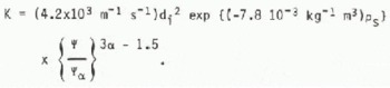
Reference WankiewiczWankiewicz (1978) has found that K varies approximately as (Ψa/ Ψ)η where η~13. Comparison with Equation (27° then gives α = -3.83. However Denoth and others (1979) find K varies as (θw/1-θj)η where η = 2.16 to 4.59. Our value of α = -0.93 implies n = 4.6.
3(d) Radiation extinction coefficients
The internal energy source SR in Equation (20) arises because short-wave radiation can penetrate for a significant distance into snow. The effects of radiation penetration are represented in the SHE model by using two values of the extinction coefficient: ν1 = 10 m−1 (short-wave), ν2 = 2500 m−1 (long-wave). Expressions for ν in terms of grain size, density and water content could be devised, but given the state of the data (Reference MellorMellor 1977), this does not seem to be justified. The use of two different values of v means that the net radiation has to be divided into short-and long-wave components. If these are not measured directly but global radiation is known the net shortwave component is estimated using the short-wave albedo.
4. Boundary Conditions
The energy flux across the upper boundary of the snowpack is
where R (the net radiation) represents the input of energy per unit time per unit area, C is the heat gained by convection from the air, r is the heat gained from precipitation and –LivE is the heat gained from condensed vapour. Assuming that the meteorological data available, for example from an Institute of Hydrology automatic weather station, will be precipitation 0 and” wind speed W, air temperature Ta, specific humidity qa, and net radiation, all measured at a height Z* above the ground, the heat input from convection may be estimated as
where Ts is the temperature of the snow surface and Dn is a turbulent transfer coefficient. Similarly the evaporation rate may be estimated as
where qs(Ts) is the specific humidity of the snow surface which is saturated at temperature Ts.
For neutral conditions in the boundary-air layer the turbulent transfer coefficient is
where k is von Kármán’s constant and z0 is the aerodynamic roughness of the snow surface. However, we cannot assume that neutral conditions always exist over a cold surface like snow. One method of estimating Dh for stable or unstable conditions, used by Dunne and others (1976), is to calculate the Richardson number Ri, and correct the value of Dh for neutral conditions by factors depending on Ri. For stable conditions
and for unstable conditions
The Richardson number is
where g is the acceleration due to gravity.
At the lower boundary the conditions depend on the conditions at the upper boundary of the soil. Since water can run off laterally between the soil and snow, T or Ψ should be matched at this interface rather than ∂T/∂Z/ or ∂Ψ/∂Z.
5. Results
Data to test the model have been collected at a site in the Cairngorm Mountains, Scotland (57°7’N, 3°40’W). The site lies at an altitude of 650 m a.s.l. on a moderate slope (zenith angle 16°) facing northwest (slope azimuth 280°). The vegetation is predominantly heather. Hourly values of meteorological data were recorded using an Institute of Hydrology automatic weather station. Temperatures were measured at five depths in the snow using thermistor probes.
First tests of the model have been carried out using 297 h of these data. The period chosen (0800 h, 21 February 1979 to 1700 h, 5 March 1979) began with three days of near-freezing air temperatures during which the snow was ripe but little melting took place. The air temperature then rose to around 4°C for a period of 3.5 d during which there was rapid melting. At 2200 h on 27 February (t = 158 h) the air and snow temperatures fell sharply and the snow cover only returned to 0°C for 2 to 3 h at 1200 h the following day. There was some melting. The snow temperature then fell again over the next night to reach a maximum at 0700 h on the following morning. Over the next two days the air temperature increased to a maximum of 8.5°C at t = 223 h. During this period there was rapid snow-melt. The air temperature then dropped back to near 0°C and snow fell from t = 258 h to t = 264 h on the following day. Such a period of rapidly changing temperatures and alternating melting and re-freezing provides a very good test for the model.
At the beginning of the period the snow cover was SO cm deep and five thermistors were buried in it, at heights of 8, 21, 27, 35 and 40 cm above the ground. The time when each of these probes became exposed to the air is clear from the temperature record so the snow depth Z is known at six times during the period, The efficiency of the model in predicting snow-melt can be determined by calculating the normalized root mean square error function
where Z is the mean of the measured values, Zi, and are the values of snow depth predicted for the same times by the model. Unless all the Zi are, like the Zi, multiples of δz, which is the finite-difference grid step used in the node!, the minimum value of (F*)1/2 will not be zero. For δζ = 5 cm, for example, (F*)1/2 min = 0.09. The same error function can, of course, be calculated for other snow-melt models run on the same data; for example, the best (i.e. minimum) value for (F*)l/2 which could be obtained using a degree-day model was 0.8 and using an energy budget model, 0.25.
The aim of these first tests was to determine how well the distributed model would perform using parameter values specified a priori rather than determined by optimization. The data needed to run the model are: initial values of temperature, density and grain size, a value for temperature at the snow-soil boundary and a value for the aerodynamic roughness. Snow-pit measurements gave ρ(z, 0) = 500 to 550 kg m−3 and d(2, 0) = 1 to 2 mm for all z. The initial temperatures recorded by the thermistors were used to construct an initial temperature distribution T(z, 01. There was some uncertainty in this, especially near the boundaries where the curve had to be extrapolated. The temperature T(0, t) was estimated to be constant and in the range -1.4 to -0.8°C, although at the end of the period, when the snowpack was only 15 cm deep, the temperature at the lower boundary must have varied. Field measurements of z0 from wind profiles over snow have ranged from ID−3 to 10−2 m. However, there has been some suggestion (Hogg and others 1982) that the appropriate value for the turbulent transfer Equation (29) and Equation (30) is much lower, that is, in the range 3x10⁻⁶ to 10−4 m. At ten different sites in the
Cairngorms the best values of the aerodynamic roughness found by optimising an energy-budget model were found to lie in the range 4.1x10⁻⁶ to 1.4X10⁻⁴ m.
Figure (1) shows the variations of (F*)1/2 over the estimated range of T(0, t) for zo = 10−3 m, ρ(2, 0) = 550 kg m -3 and d = 1 and 2 mm. The predicted snow depths are not very sensitive to the choice of lower boundary conditions except at the end of the period. Thus for these data it is not so important to know the lower boundary condition accurately. Figure 2 shows the variation of (F*)1/2 over the range zo = 10−5 to 10−3 m for T(0, t) = 1.2°C, and ρ(z, 0), d(z, 0) in their measured ranges. It is clear that the model predictions are highly sensitive to changes in z0.
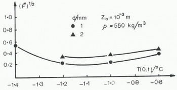
Fig. 1. Variation of the normalized root mean square error function with temperature at the lower boundary of the snow cover.

Fig.2.. Variation of the normalized root mean square error function with aerodynamic roughness.
The best value of (F*)1/2 achieved with the distributed model using a grid spacing of Δz = 5 cm is the minimum possible value, 0.09. This is well below the best values achieved using the energy-budget and degree-day model. Thus if one parameter alone is optimized in all three models, to make the comparison of performance fair, the distributed model is clearly the best for the Cairngorm data and the degree-day model is the poorest. The optimum value of zo = 5 × 10⁻⁴ m for ρ(z, 0) = 550 kg m−3, d(z, 0) = 1 mm and T(0, t) = 1.2°C falls between the range suggested by Hogg and others (1982) and the range given by wind-profile measurements.
Figure 2 shows the importance of being able to specify z0 for good snow-melt predictions. Further research into turbulent transfer over snow is needed so that values for this parameter can be determined a priori with as much precision as those for the other parameters of the model.


