


INTRODUCTION
Continuous, nonlocalized flow velocity measurements in dense flow avalanches, as well as at least localized flow depth and flow velocity profile measurements perpendicular to the slope, are needed to further investigate the flow characteristics of avalanche snow from start to stop of dense flow avalanches. Flow velocities in the front, the body and the tail portion of the avalanche have to be measured even if a snow dust cloud inhibits the optical view on the flowing part of the avalanche. To be able to separate the influence of snow quality from the influence of track geometry on the flow mechanism, the measuring system has to allow measurements at different tracks on the same day with similar snow conditions as well as measurements at the same track under different snow conditions. The technical specifications that fulfill the above stated requirements are listed in Table 1.
CONTINUOUS WAVE DOPPLER RADAR FOR VELOCITY MEASUREMENTS
Preliminary experiments and investigations showed that microwave doppler radar is the most promising tool for measuring avalanche speeds. The flowing snow itself acts as a radar target that reflects part of the microwave signal back to the transmitter-receiving antenna system. The relative motion of the snow to the radar antenna causes a frequency shift between the transmitted and the reflected signal. This frequency shift fD (doppler shift) is given by

where fo is the frequency of the continuously transmitted microwave signal, f R the frequency of the
Table 1. Technical Specifications Of A Measuring System To Investigate Flowing Avalanches

reflected signal,![]() the target position vector relative to the transmitter-receiver position,
the target position vector relative to the transmitter-receiver position, ![]() the target velocity vector, and c the velocity of light. If α is the angle between the target position vector and the target velocity vector, Equation 1 reduces to
the target velocity vector, and c the velocity of light. If α is the angle between the target position vector and the target velocity vector, Equation 1 reduces to
DENSE FLOW AVALANCHE AS A RADAR TARGET
The microwave reflectivity of snow (1-30 GHz) is dominated by surface scattering for nearly rectangular incidence and by volume scattering for incidence angles deviating more than some 10° from rectangular incidence. Volume scattering in homogeneous dry snow is very low; penetrability equals many wave lengths. In wet snow absorption is high and penetrability is limited to about 1 wavelength.
Mätzler and Schanda (1984) measured the X-band (10.4 GHz) backscatter coefficient y of natural dry and wet snow covers as a function of the nadir angle (nadir angle θ = 0 for surface rectangular incidence). Equation (3) relates γ to the well known radar cross section σ0.
Only for nadir angles below 20° did these measured reflectivities of dry snow cover exceed that of bare ground. For larger nadir angles dry snow cover was almost transparent. Matzter and Schanda estimated a penetration depth of 10 m in dry snow. Ulaby and others (1980/82) made similar experiments. They found a significantly reduced penetration depth in a non-homogeneous snow cover piled up manually.
Wet snow is not transparent at X-band frequencies. For nadir angles between 20° and 70°, γ decreases from -lOdB to -20dB, decreasing further at grazing incident angles.
Avalanche snow consists of a mixture of snow blocks, rounded snow chunks and fine grained snow. Debris size and surface roughness often have characteristic lengths comparable to the wave length of X-band radars (0.03 m). The refractive index of dry snow is about 1.3 (ρ = 350 kg/m3). For wet snow the real part of the refractive index may be significantly higher depending on wetness. Targets of this type (Mie to optical scattering range) have a reflectivity which is roughly constant for a wide range of incidence angles with theoretical values of γ of the order of -lOdB to + 10dB. Estimated values from experiments for small avalanches are in the range of 0 to + 10dB.
Backscatter from snow particles suspended in air is small for two reasons: the backscatter of the individual ice particles (diameter - 1mm) is small (-30dB), and the density of the air snow mixture is low (a few kg/m3). The experiments confirm that flowing snow can be recognized by X-band radar even through the well-developed dust cloud of a powder snow avalanche.
DOPPLER RADAR AND FMCW RADAR TECHNIQUES
For simplicity we use continuous wave doppler radar. The useful frequency range is limited by time resolution, velocity resolution, spatial resolution, frequency dependence of the target cross section of avalanche snow and system availability. The target velocity distribution results from the Fourier Transform of the time domain doppler shift signal (frequency difference between transmitted and received microwave signal) into the frequency domain.
Table 2. Doppler Radar Specifications

The length of the time domain window (length of analog signal train) chosen for the Fast Fourier Transform (FFT) determines maximum time resolution for independent velocity spectra (FFT performed on non-overlapping periods of the time domain signal). Window width and shaping determine also the velocity resolution. For the simplest case of a uniform windowing function, a time domain record length of 100 ms corresponds to a -3dB frequency resolution of 10 Hz. If we require a velocity resolution better than 0.5 m/s we have to obtain a doppler coefficient 2 f0/c of at least 20 m-1 (Equation 2). This corresponds roughly to a transmitting microwave frequency of 3 GHz. At this frequency parabolic antennas with a diameter of about 3 m have to be used to obtain the required spatial resolution (Table 1). Antenna diameters above about 1 m are not suitable for relocatable field experiments. We decided therefore to choose transmitting frequencies above 9 GHz. For the target reflectivities estimated in the preceeding paragraph and radar ranges up to 2000 m, transmitting powers of a few hundred milliwatts are required to get a reasonable backscattered signal in a simple low-cost continuous wave radar system. Because of the availability of cheap "off the shelf microwave components, especially semiconductor oscillators with output powers up to 500 mW, we decided to start the experiments using X-band (8-12 GHz) radar systems. In this frequency range the required velocity, spacial and time resolutions can be achieved and the penetration depth is still reasonable.
The specifications of the 5 X-band doppler radar channels available for simultaneous operation from oversnow vehicles are listed in Table 2. Figure 1 shows a block diagram of the monostatic and bistatic systems developed for the avalanche speed measurements.
Depth of the avalanche flow is measured locally by fmcw-X-band radars buried in the ground under the avalanche track, looking upward at 90° to the flow direction through the static part of the snow below the sliding plane, and through the moving avalanche snow above the sliding surface. The radars continuously measure the electro-magnetic distances between the ground surface, the sliding layer and the moving chunks of snow. The basic time resolution is 25 ms. The distance resolution for static targets is 0.03 m, for targets moving perpendicular to the radar beam, because of the finite antenna aperture and doppler broadening, about 0.1 m.

Fig. 1. Basic setup for avalanche flow speed and flow depth measurements.
To estimate geometrical distances, mean densities of the flowing snow have to be measured or estimated. A more detailed description of the fmcw radar is given by Gubler (1984).
TEST SITES
For system development, tests and first measurements, small avalanche tracks in the vicinity of our Institute (2700 m a.s.l.) were chosen. These tracks have drop heights of 150 m to 400 m and track length between 400 m and 700 m. During the winter 1983/84 for the first time speed measurements were performed on the Lukmanier Pass at the north south divide in Central Switzerland. This pass (1400 - 1600 m a.s.1.) is closed during winter because the highway is endangered by many large avalanches with drop heights of 600 m to 1200 m and track lengths of up to 2.2 km. Some of these avalanches run up to 5 times per winter. For our purpose the avalanches are released artificially using mortars and bazookas.
DATA ANALYSIS AND REPRESENTATION
Besides the on-line avalanche speed determination, the doppler and the fmcw mixer output signals are stored by an analog tape recorder. The data is Fourier transformed off-line with corresponding real time resolutions of 25 ms for the flow height spectra and 125 ms for the speed spectra. Up to several thousand spectra have to be stored per channel and per avalanche for further processing. To enhance the spectra different types of noise reduction techniques are applied; averaging, subtraction of synthetic or measured noise spectra, restoring the original signal amplitude range etc. The resulting doppler spectra show the momentary distribution of speeds of the snow targets illuminated by the radar. The further interpretation of the speed spectra therefore depends on the footprint of the radar. Narrow beam radars deliver time profiles of the avalanche moving through a given location in the track, whereas wide angle antennas deliver a combination of target speeds as a function of time occuring in a large fraction or even along the whole track (Figure 2). Narrow beam systems measure the variation of snow speed from avalanche front to tail and allow an interpretation of the wide angle radar spectra. So far all avalanches measured showed their highest speed immediately behind the front (Figure 3). For small avalanches the snow speed starts to decrease immediately behind the front, whereas for large avalanches the snow speed remains at its highest level for a certain time (avalanche core) before tailing off. This fact allows the identification of the maximum speed occuring in the wide beam angle radar spectra with the avalanche front speed. Knowing the slope parallel avalanche front speed as a function of time as well as the starting position of the avalanche, the front speed can be determined for every location in the track from start to stop on the basis of a digitized length profile of the avalanche track (Figure 6).
The height above ground of the sliding plane and the flow speed are deduced from the fmcw radar spectra (Figure 4). Partially semi-interactive computer codes have been developed for the interpretation of the enhanced spectra. The relatively high time resolution of the flow height measurements of 40 spectra per second allows one to autocorrelate time series of spectral amplitudes for a given height above ground and to crosscorrelate similar time series of two different synchronized radars which are operated a few meters apart in the main flow direction (Figure 1). The autospectra give information on structural features of the flow at a given height whereas the cross-spectra give information on the propagation time for the features at a given height from the first to the second radar. An example for a cross-spectrum is given in Figure 5. If cross-spectra are determined for different levels in the flow a rough slope perpendicular flow speed profile can be determined. Because system tests have so far been performed only in shallow avalanches, no speed profile data are yet available.

Fig. 2. a: Speed spectrum of block flow (release zone) measured with a narrow beam radar.b: Speed spectrum of a large mixed avalanche (dense flow and powder snow avalanche).

Fig. 3. Narrow beam radar speed profile (flow speed as a function of time at a given location) of a large mixed avalanche.

Fig. 4. Flow height spectrum: the channel number is proportional to the electromagnetic distance. The geometrical distance between the markers A and B amounts roughly to 0.3 m. The solid curve shows the situation just before the small avalanche reached the radar. The natural snow surface is just above marker A. The dashed line shows a spectrum during the flow. The uppermost layers of the snow cover are densified, the lower layers (toward the origin) remain unchanged. The avalanche slides on the snow surface. The flow height is given by the distance between marker A and B.

Fig. 5. Cross spectrum between two radars located about 8 m apart in the flow direction of the avalanche. The peak at 1.7 Hz corresponds roughly to a flow speed of I2m/s just above the sliding plane (Figure 4).
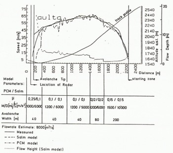
Fig. 6. Measured front flow speed of a large channeled dry snow, mixed avalanche as a function of the track location Estimated avalanche volume >I00 000 m3. flowrate 80OO m3s. The flow has been simulated using traditional avalanche models.
SIGNATURES OF LOCAL FLOW SPEED DISTRIBUTIONS
Our first experiences indicate that speed spectra show distinct signatures for different types of avalanches and also for different portions of the avalanche track. Small slab avalanches mainly consisting of block flow (sliding of the slab broken into parts), block flow in starting zones, and sheet flow (locking of part of the avalanche snow into down-slope moving solid slabs or sheets) in rounout zones produce fairly narrow, almost symmetrical spectra.
Track flow for fully developed avalanches is characterized by wider spectra which often show a sharp cutoff at the high-speed end, followed by a wide maximum toward lower speeds and long tails often reaching down to zero speeds. Mixed avalanches with a well developed snow cloud often tail off toward higher speeds above the characteristic cutoff speed. We interpret this part of the spectrum as a contribution from the well developed powder snow avalanche.
COMPARISON OF MEASURED FLOW WITH TRADITIONAL AVALANCHE MODELS
The two models used in this comparison are: the PMC of Cheng and Perla (1979), which is essentially the original Voellmy model, and Salm's model (1979) which is a Voellmy model that includes continuity, assuming steady flow in the track and position independent nonsteady flow in the runout. The computer code applies the basic equations of the two models consecutively for small segments of the track allowing for different types of crosssection characterisations (V-shaped, rectangular, shallow slab) and for varying model parameters along the track. The main parameters of the two models are: Avalanche rnass M (PCM) or flow rate Q (Salm), Coulomb friction coefficient μ, and a coefficient of a friction term proportional to the speed squared named either drag D (PCM) or ![]() (Salm).
(Salm).
Figure 6 shows flow simulations for a large avalanche. The main conclusion from this modelling calculation is that a low Coulomb friction term has to be chosen to get the high speeds measured. The importance of the speed limiting "turbulent" friction term has to be limited to very high avalanche speeds. The Salm model results in much shorter relaxation distances, the avalanche speed is very sensitive to changes in slope angle or track width, whereas the sliding mass model (PCM) produces only gradual changes in speed.
This fact often requires a drastic change of the parameters in the runout zone for the PCM model to stop the avalanche at the required position. Improved models that take different flow mechanisms for different sections and flow regimes of avalanches into account are discussed in the next paragraph.
FLOW PATTERNS OF AVALANCHING SNOW
The aim of the following sections is to develop some new ideas for the mechanics of flowing avalanches to achieve a better understanding of the presented measurements. From qualitative observations it seems evident that an avalanche passes through different stages of flow patterns, from the start in the fracture zone, to the track, and to the standstill in the runout zone. Hitherto for the whole movement the same mechanical model has been used, mostly the Voellmy model (Voellmy 1955), the similar and refined PCM and Salm models, or that of Brugnot and Pochât (1981).
When an avalanche starts as a snow slab, the principal movement is pure sliding of large blocks on the bed surface. With acceleration and increased roughness at the base it splits into smaller blocks, which then begin tumbling and colliding. In certain circumstances the blocks disaggregate into smaller clods, performing irregular motions over the full flow depth. In the zone of deposit these motions disappear gradually until again a pure sliding may be reached. If an avalanche starts in a loose-snow manner, irregular movements seem possible from the very beginning.
To get more insight into these phenomena the movement of a granular material has to be considered, abandoning the hydrodynamical point of view. During the last few years research in this field has seen rapid progress (see eg Scheiwiller and Hutter 1982). Because of enormous mathematical difficulties, analytical solutions are rare and exist only for very simplified assumptions of material behaviour and flow geometry. Although such solutions may be unrealistic for practical purposes, they can give valuable insight and be used in a more qualitative way.
THEORETICAL CONSIDERATIONS BY HAFF
Recently Haff (1983) studied the movement of a granular material from a continuum point of view, ie individual grains are treated as "molecules" of a granular "fluid". In addition to the flow velocity u, a mean random fluctuation ("thermal") velocity v of individual grains has to be introduced. Grain-grain collisions are inelastic and the average separation distance of grain surfaces s is much smaller than the grain diameter ϕ; conditions which are probably fairly well obeyed in flowing avalanches. More questionable are assumptions of lacking cohesion or sintering among grain surfaces and the neglect of grain spin.
To get a qualitative insight into different flow patterns we will use the analytical solution for steady state Couette flow with no gravity by Haff (1983).
From the momentum equation (Navier-Stokes equation) it follows that the pressure
is constant, where t is a dimensionless constant and p the bulk density assumed to be approximately constant. The same is true for the shear stress

with q being a dimensionless constant and  gradient of the flow velocity perpendicular to the plates (y-direction). The expression

represents the "viscosity"-coefficient.The energy equation reduces in that case to

Subscript 1 means the x-direction parallel to the plates, and 2 is in y-direction. K functions like a thermaldiffusivity since the internal energy  behaves like a "temperature" of the system, when this energy corresponds to "kT" (Maxwell-Boltzmann). The parameter K can be expressed by

where r is a dimensionless constant. The quantity I represents the energy lost through collisions per unit volume per second

due to inelasticity of collisions, y is a dimensionless factor proportional to (1-e2), with e being coefficient of restitution (e = 1 for elastic grains).
From Equation 7 we get the differential equation

with the "frequency"

which can be either positive or negative. When it is negative, the curvature of v between the plates is positive and the solutions are exponentials. With positive w2 oscillatory solutions with negative curvature are obtained.
The criterion for the two solutions is the ratio of frictional to collisional energy loss rates. The first is given by the "viscosity" of the material amd amounts to

and the second is given by I. Therefor

where

is a length scale, expressing the distance over which v is maintained, eg in a steady-state system with no flow u, when energy is conducted from outside into the volume by vibration of the bottom plate.With negative w2 and the boundary conditions (h is the plate separation
and
the following solutions are obtained:


>The quantity

is giving the total of "free-space" between grains. The given "thermal" velocity v 0 originates from an induced vibration of the bottom. According to Equation 20 most of the grains move as an essentially non-deforming plug with the exception of a layer of thickness ≃λ. In such a case the material is partly fluidized.
With positive w2 shear stresses dominate over the whole volume and with this enough thermal energy is produced in the grain system. The material is fully fluidized and considerable velocity gradients occur over the whole flow depth.
With the boundary conditions
>the following solutions are obtained


NECESSARY ADAPTIONS FOR APPLICATION TO FLOWING AVALANCHES
It is clear that above assumptions do not all fit the real conditions of an avalanche: it is not a Couette flow without gravity, the boundary condition U(o) = o may not be fulfilled in many cases and in the interaction between grains one has at least - besides the effect of collisions -to assume Coulomb friction among "grains".
In the presence of gravity - as demonstrated by Haff (19832 for PerfectIy elastic grains - both velocity profiles for v and u are deformed compared to those without gravity. The fluidization is more pronouced near the upper plate and the pressure p is only in its first approximation proportional to U2, whereas shear stress remains proportional to U2
Observations in runout zones show in most cases a stand-still on slopes inclined downhill in direction of movement, which is only possible with an existence of velocity-independent friction forces. Laboratory experiments by Lang and Dent (1983) indicate that Coulomb friction can be assumed for this force. In the energy Equation 7 the term representing the power of stresses due to collisions

has to be completed by the power of a friction stress ![]() constant for a given y,
constant for a given y,
which does not change Equation 13 principally.
In the solutions by Haff (1983) the boundary conditions (15) and (24) seem unrealistic at least for the case of pure sliding, which we have to introduce as a third flow pattern: the non-ftuidized one. The thermal velocity disappears everywhere and the flow velocity is constant over the full flow depth, except in a boundary layer where solely Coulomb friction occurs.
THE THREE FLOW PATTERNS OF A FLOWING AVALANCHE
In Figure 7 the possible three alternative flow patterns are plotted. A decisive point becomes now the criteria determining the flow mode. The alternation from a partly to a fully ftuidized state is given by Equation 13. The material is partly fluidized if the collisional energy loss rate exceeds the frictional one or in other words if v 0 at the ground is larger than U. In an avalanche v 0 can only be generated by the roughness of the ground which is equivalent to a vibration of the lower plate in the Couette flow experiment. Full fluidization could be reached if the grains are nearly elastic (e close to unity). For the change from sliding to the partly fluidized state, we do not have an analytical solution of a similar problem which could help at least in a qualitative sense. One can merely suppose that sliding will be maintained on smooth avalanche tracks with elevated strength of the sliding snow.

Fig. 7. The three possible flow regimes in flowing
avalanches
All these criteria are not yet well established, however the measured development of avalanche speeds will give indirect indication of flow mode. One could expect an order of flow patterns with increasing velocity: sliding -partly fluidized - fully fluidized. The interpretation of the test results indicate however, a partial fluidization even with extremely high flow velocities.
BASIC ASSUMPTIONS
We are confining our considerations to the avalanche core. The front should be treated separately, but, as with the core, probably not with the usual hydrodynamical relations.
For sliding the shear resistance at the ground is independent of velocity and is given by the dimensionless friction coefficient μ. Pressure is assumed constant and no deformations or changes in flow depth are possible in x-direction.
In the partly fluidized state, snow is disintegrated into clods much smaller than the flow depth d. With expected small e the thickness λ of the fluidized layer is small compared to d. The pressure
is constant in the fluidized layer and the speed-dependent shear stress
depends linearly upon flow velocity at the top of the flow. Both cp[m2/s2] and ca[m/s] depend on v 0, given by the roughness of the ground. Deformations in x-direction or changes in flow depth are impeded as λ is small.When the system is fully fluidized deformations or changes in flow depth - eg if the slope angle alters - are possible due to the inner mobility of clods. The pressure
and the speed-dependent shear stress

depend on the square of speed. Equation 34 is formally (but not physically) coincident with the Voellmy model, the reason why c's has been replaced by g/, the traditional notation in avalanche dynamics. The nature of pressure however differs from the usual assumption in avalanche dynamics (velocity-independent pressure as in hydrodynamics).
The equation of continuity for our nearly incompressible material can be expressed as
which says, that
with Q1 being the discharge per unit width [m3/s - /1/m] and u the mean velocity over flow depth d
The equation of motion in the large is obtained by integration over a fixed region in space of height d and unit length and width. It reads as follows:

where ψ represents the slope angle and T(U) the velocity-dependent shear stress. Equation 37 is based on an averaged velocity u. It will therefore contain certain errors which increase the more the velocity profile deviates from a rectangular one (corrections can be made as soon as we shall know more about profiles from future field tests). Furthermore a nearly uniaxial movement is assumed ie

AVALANCHE MOVEMENT IN THE THREE FLOW REGIMES
For sliding we obtain from Equation 37

because Assuming constant ψ, integration of Equation 38 yields
with
and uo being the initial speed at x = o .With tg+ = μ a steady movement u = uo = const occurs. For a the movement is slowed down by

and a standstill of the front particles is reached at

For partial fluidization Equation 37 becomes
because of ![]() – fulfilled for λ » d – and
– fulfilled for λ » d – and  .
.
Integration of Equation 43 yields with constant ψ

with

For a the movement accelerates, and a maximum speed °f a d

Can be reached, therefore u0 ≤ u ≤ umax.
For a the movement is slowed down and standstill of front particles is reached at

As the material is only partially fluidized the flow depth should remain the same before and after ($?ηψ -μθθ?ψ), changes its sign. This however may be questionable in case of long avalanches, where back parts of the avalanche hit the front parts already slowed down. Then a pressure P per unit width

approximately calculated from the momentum theorem, may either deform the snow over a certain distance and increase d proportionally to u2/2g or, if the strength of snow is high enough, push the front snow forward causing much longer runout distances than predicted by Equation 47.
A further possibility may be that the snow-body breaks up and the following part turns aside forming a different runout path (the same may occur in the non-fluidized state of sliding).With full fluidization the material behaves more like a fluid. For an avalanche not too short in length and if starting and runout is excepted, a stationary movement may be reached for a certain while. This is supported by our measurements (see Figure 3). Equation 37 becomes

Using the equation of continuity (36)
we get the differential equation for stationary, nonuniform flow

where uu is the constant velocity reached at a lower part of the track with a slope angle ψ? (uniform flow). B is the width of the (unchanneled) avalanche and ' _ (1 -2c' )
The traditionally used formula for the runout distance of the front particles (Salm 1979)

with V2 = daξ(μcosψ − sinψ) and da being the mean deposition depth, can probably not be used in most cases because full fluidization over the whole runout is hardly imaginable. With strong retardation compressive forces will increase internal friction and sintering, so that the mobility of clods is considerably reduced (similar effect as gravity in Haffs (1983) theory).
CHECK OF THE MODELS BY OUR MEASUREMENTS
In Figure 6 a comparison was made between measurements and two conventional models. Both models are (tacitly) based on a fully fluidized flow regime. As it is demonstrated, a fit is naturally possible with the two free parameters. Unsatisfactory are however the facts that the "constants" had to be altered considerably over the track and the {-values (Salm model) had to be assumed about ten times larger than it was usually done so far. Furthermore the extremely low μ-values seem nearly unrealistic.
In Figure 8 an attempt was made to fit the measurements of the same avalanche as in Figure 6 with the proposed movement in different flow regimes.

Fig. 8. Aulta avalanche of 8 February 1984. Comparison of measurements with different flow regimes. S means sliding and PF partly

Fig. 9. Aulta avalanche of 10 February 1984. Comparison of measurements with sliding flow regime (S).
In the first part of the track (2250 m to 2050 m) the best fit was attained in assuming sliding. A direct determination of u. was therefore possible. Striking is the sudden change of acceleration at 2050 m on the same mean slope angle. This can now easily be interpreted as the change from sliding to the partly fluidized state.
From 1450 m to 1050 m acceleration decreases again due to the lower slope angle.
The situation in the two sections from 1050 m to 800 m and 800 m to 320 m is not so clear.
Due to the pronounced channeled track and the reduced slope, the flow depth increased gradually in contrast to the assumed partly fluidized state. Here merely umax was calculated.
In the runout, beginning at 320 m, the partly fluidized regime gave the best fit although the theoretical runout distance is about twice as long as the observed one. Fortunately this can easily be explained by the strong lateral spreading of the avalanche.
The change of factor b can be seen as the influence of varying flow depth and not as a change in ca In any case the flow depths determined in that way are in fair agreement with observations.
The whole avalanche from the start to the stop could therefore be modelled by constant values of μ and ca. The reason why full fluidization was probably never reached is not clear, may be it was because of a pronounced inelasticity of snow clods or even that this regime can hardly be attained in flowing avalanches.
In Figure 9 the runout of the Aulta avalanche of 10 February is modelled by sliding, delivering the best fit to the measurements of this relatively small avalanche. The decrease of u in the lower section could be explained with increasing flow depth (in contrast to the sliding regime).


