


Introduction
The radar altimeter aboard Seasat was designed to measure ranges to the ocean surface. It transmitted short radar pulses with a beam width (to 3 dB attenuation) of 1.6 degrees of arc. Pulse length was 3.125 ns (equivalent to -1 m), and pulse rate was 1 020 s_1. Ranges were obtained from the time delay between pulse transmission and receipt of the reflected pulse. Return energy was measured during a data-acquisition window of about 188 ns duration. High resolution was achieved by dividing this window into 63 time gates. In operation, the altimeter initially undertook a low-resolution search for the ocean surface, and then located the center of the high resolution acquisition window to coincide with the time of the return-pulse leading edge. Thereafter, the altimeter maintained track of the ocean surface by continually adjusting the timing of the acquisition window as dictated by the rate of change of previous measured ranges. The tracking worked well over the oceans, where measured ranges changed very slowly. However, over sloping or undulating terrain, the servo-tracking circuit was not sufficiently agile to monitor the rapidly changing ranges, and the altimeter frequently lost track of the return pulse. This resulted in short periods (usually a few seconds) when no useful data were obtained. Nevertheless, more than 600 000 surface elevations were measured on the portions of Greenland and Antarctica that lie between ±72° latitude. These are undergoing systematic correction for tracking errors and slope-induced errors as part of the research program of the Oceans and Ice Branch at the Goddard Space Flight Center (Zwally and others in press).
In this paper, we show how radar-altimetry data can be used to map i ce-sheet margins. Seaward ice fronts of the ice shelves, and ice margins generally, are associated with a step change in surface elevation. Mapping the ice front would be straightforward if the altimeter responded immediately to the abrupt change in surface elevation. However, the Seasat radar altimeter responded slowly and usually lost track for a few seconds. Nevertheless, the ice-front position can be inferred accurately from the relationship between satellite position and measured range prior to losing track. As the satellite passed over the ice front from seaward, it continued to record the return signal from the sea, or sea ice, that lay within the seaward portion of the beam-limited radar footprint (radius approximately 11 km). Consequently, the measured range was the oblique distance from the satellite to the sea surface next to the ice front. The variation of measured distance with time gives the ice-front position to within 100 to 1000 m, depending on data quality and the length of time during which oblique ranges were measured. In addition, the data give an indication of the shape of the nearby ice front as related to the orbit track.
When the satellite crossed the ice front travelling seaward, oblique ranges were similarly obtained to the nearest portion of ice shelf. Seasat crossed the Antarctic coastline at more than 1 000 points which are, on average, 7 km apart. Crossing-point coordinates resulting from analysis of all the altimetry data would represent the best available mapping of the East Antarctic coastline. Comparison of the coastline with earlier maps or future surveys would reveal changes in the ice margin.
Method
Figure 1 shows a sequence of radar-altimeter measurements as the satellite passes over an ice front. Initially, reflected energy is received from the horizontal sea-ice surface (Fig.1.(a)). The portion of the radar footprint shown in the figure represents the maximum area from which energy is received during the 188 ns data-acquisition window. This acquisition footprint is a circle with radius of approximately 5 km represented by the cross-hatched area in Figure 1(a). The dark region at the center of the circle represents the pulse-limited footprint (PLF) which is the maximum area from which energy is simultaneously received as the radar pulse first illuminates the surface (Brooks and others 1978), The radius of the PLF is determined by satellite elevation, pulse length, and surface roughness. Over a smooth surface, it is typically 0.8 km in radius. The reflected pulse received by the altimeter is also shown in Figure 1(a). The initial, rapid rise in received energy corresponds to total illumination of the PLF by the transmitted pulse. Thereafter, the energy intensity decreases rapidly to yield a sharp pulse shape indicating a specular reflection, which is characteristic of sea ice. This specular reflection differs markedly from the diffuse reflections characteristic of oceans and the firn on ice sheets; these generally possess a sharp rise but slow decay.
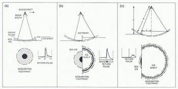
Fig. 1. Radar altimeter approaching an ice shelf and continuing to measure ranges to nearby sea ice after crossing the ice front. The radar pulse is of very short duration and is represented by the solid line. The acquisition footprint (cross-hatched area in (a)) indicates the area from which reflections can be received during the data-acquisition window (of duration 2t). The pulse-limited footprint (-1 km radius) is the black area; the area from which reflections are received prior to the main return is double cross-hatched; the area contributing to the trailing edge of the return pulse is single cross-hatched, c is the velocity of light.
Examples of Seasat radar return pulses over sea ice are shown in Figure 2. Onboard processing of the data included summing of 100 successive return pulses to produce a composite pulse shape giving an average representation of the data collected during 0.1 s. The summing process involved offsetting successive pulses to correct for changes in range that occurred between pulses. This was achieved using a predicted range rate based on past observations. Inevitably, this introduced errors which caused slight stretching of the composite-pulse rise time. However, this disadvantage was more than balanced by the improvement in signal to noise ratio achieved by summing the 100 pulses. The twin-peaked pulse in the fifth frame of Figure 2 is a result of the averaging process. The altimeter obtained the composite pulse by first summing two successive sets of 50 pulses, and then summing the two resulting pulses. Occasionally, errors in predicted range rate resulted in a significant offset between the two 50-pulse composites, yielding twin spikes as shown in Figure 2.
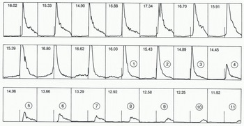
Fig. 2. Reflected radar pulses obtained at intervals of 0.1 s by the Seasat altimeter as it approached from seaward, and then crossed Amery Ice Front. Each frame represents a time window of duration of about 188 ns, equivalent to an elevation difference of about 28 m. The numbers in each frame give the altimeterderived surface elevation in meters above the ellipsoid. This elevation, before correction for lags in the tracking circuit, corresponds to the time of the short vertical line in the center of the window. Frames (1) to (11) represent oblique ranges to sea with the satellite over the ice shelf.
Figure 1(b) shows the altimeter directly over the ice front. The PLF now consists of a (dark) semicircle on the sea ice and a thin semicircular stripe on the ice shelf. The ice front acts as a shutter, reducing the size of the PLF on the sea ice. The total area interrogated during the data-acquisition window is now divided between sea ice and ice shelf. As the ice front is approached, however, the edge of the radar beam encounters the ice-shelf surface before the radar pulse reaches the sea ice, and this results in a return signal prior to the arrival of the specular reflected pulse. The double cross-hatched area in Figure 1(b) represents a portion of the ice shelf which is closer in range and from which energy is received during the first half of the data-acquisition window. Over sea ice, no energy is received during this period, unless icebergs are present providing a surface closer in range within the field of view.
Finally, in Figure 1(c), the altimeter is over the ice shelf and it continues to measure ranges to the sea ice near the ice front. The altimeter has not responded to the abrupt change in elevation at the ice front. Energy reflected from the sub-satellite position on the ice-shelf surface is received before the sea-ice return, but it arrives too early to be included within the data-acquisition window, which detects only reflections from the double cross-hatched portion of Figure 1(c) before the arrival of the relatively stronger sea-ice return pulse. The seaice reflection is stronger for two reasons: sea ice is a good reflector, and the sea-ice PLF is closer to the center of the radar beam (and therefore less attenuated by the antenna gain pattern) than the shaded region on the ice shelf. Similarly, as the cross-hatched region migrates towards the edge of the beam, the intensity of the pre-pulse return decreases. The measured range increases (yielding progressively smaller apparent surface elevations) as the satellite travels inland. Indeed, the measured range increases too rapidly for the servo-tracking circuit, and the return pulse migrates to the right of the data acquisition window. This sequence is shown in Figure 2, which is a set of return pulses fron a Seasat orbit passing over Amery Ice Shelf (Fig.3.). The first seven frames show typical sea-ice specular return pulses. The next four frames also show specular reflections, but they include reflected energy within the first half of the frame. This is caused by oblique reflections from the cross-hatched portions of the ice shelf shown in Fiqure 1(b). The series of frames labelled (1) to (11) show the obliquely reflected, progressively weaker pulses from the sea ice as the satellite travelled inland from the ice front.
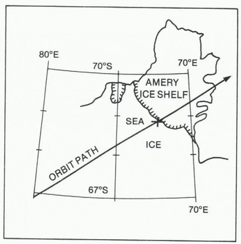
Fig. 3. Seasat orbit 2-216 passing over Amery Ice Shelf. The cross marks the ice-front position derived from the altimetry data.
The numbers at the top of each frame in Figure 2 are the altimeter-measured ranges expressed as surface elevations in meters above the Earth ellipsoid. These measurements must be corrected for tracking errors by measuring the offset between the tracking line (in the center of the frame) and the threshold of the return pulse. The threshold is found by extrapolating downward, into the pre-pulse noise, the steeply-rising leading edge of the return pulse. Correction for the offset gives the apparent elevation of the portion of the PLF that is closest to the altimeter. This differs from normal practice, which is to measure the offset to a point halfway up the leading ramp, and thus obtain the average apparent elevation of the PLF. Here, we measure to the threshold of the return pulse to ensure that our measurements refer to the portion of sea ice closest to the ice front. For the oblique ranges, this becomes an important distinction, because the obliquely-scanned PLF continues to increase in area after initial illumination by the transmitted pulse, resulting in progressively longer rise times for the oblique return pulses, as is shown in Figure 2. For pulse shapes havig twin spikes (as in the fifth frame of Figure 2) the corrected range was obtained using the average offset between the tracking line and the thresholds of the two spikes.
Figure 4 is a plot of correct apparent surface elevation against distance along the sub-satellite track. For the first 10 km the measurements were unaffected by the ice front ; in this region tilt and undulations in the apparent surface are possibly caused by measurement errors, sea-ice thickness variations, undulations in the Earth geoid, or deviations in the ocean surface from the geoid. Some of these features may yield glaciologically useful information, and they are now under investigation by the authors. For the purpose of this paper, we shall assume that the geoid, inland of the ice front, can be represented by the broken line in Figure 4. The data points marked (1) + (11) appear to have surface elevations lower (by Δ) than the geoid. They represent oblique-range measurement to nearby sea ice, with range increasing and apparent elevation progressively decreasing as the satellite moved inland (Fig.1.(c)). The distance x to the ice front from each sub-satellite position corresponding to these 11 data points can then be calculated from the relationship:
where E is satellite elevation above the geoid (-800 km) and R is the measured oblique range to sea ice (Fig.1.(c)). The decrease in apparent surface elevation is defined as Δ(=R-E). Because ?»Δ, Equation (1) can be simplified to:
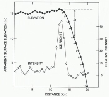
Fig. 4. Apparent surface elevation versus distance along the sub-satellite track for an orbit crossing Amery Ice Front. Also shown is the average intensity, in arbitrary units, of the pre-pulse radar reflection.
Results
Solution of Equation (2) for each of the data points (1) to (11) gives a set of circles of radius x centered on each sub-satellite point. The portion of ice front nearest to a given sub-satellite point lies somewhere on its circle. The envelope described by the 11 circles then gives a mapping of the ice-front position (Fig.5.). If the sub-satellite track is not perpendicular to the ice front, the points to which oblique ranges were measured do not lie on the subsatellite track. In these cases, there is an ambiguity in the mapping, since the ice front could lie either to the left or right of the orbit track, but this can generally be resolved by comparison with existing maps, or by continuity between ice-front sections obtained from adjacent orbits. The possible ice-front configuration shown in Figure 5 includes several embayments. The embayments are suggested because circles for three or more adjacent sub-satellite points tend to intersect at discrete points, which may be preferred radar reflecting sites. Many ice fronts are irregular, and embayments containing sea ice provide the most likely explanation.
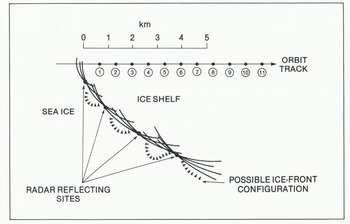
Fig. 5. A portion of Amery Ice Front derived from radar-altimetry measurements.
Errors in calculated ice-front position result mainly from errors in Δ (the decrease in apparent surface elevation). For this example, we assume this error to be ± 0.5 m. The corresponding error fix in calculated distance from sub-satellite point to the ice front is shown in Figure 6. For the point closest to the ice front, the error is large (-±1 km), but decreases rapidly to less than ±200 m for points (4) to (11). Errors in sub-satellite position contribute an additional uncertainty of less than ±10 m to the calculated ice-front position. The cross in Figure 3 marks the calculated position of the ice front. It is about 5 km to seaward of the ice front depicted in the map, which is based on data obtained during the 1960s.
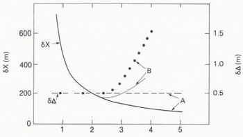
Fig. 6. Errors in ice-front mapping. “A” refers to data obtained crossing Amery Ice Front from seaward; “B” refers to data obtained crossing the Fimbul ice front from inland.
The intensity of the reflected radar signal that arrives before the main sea-ice return should increase as the ice front is approached, due to reflections from the top of the ice shelf. A full description of the behavior of this pre-pulse return is beyond the scope of this paper. For the present, it is sufficient to note that for a flat, horizontal ice shelf the intensity should increase to a maximum when the satellite is a short distance inland from the ice front. Thereafter, the pre-pulse intensity should slowly decrease. In Figure 4, the average return-signal intensity for the first 27 of the 63 gates comprising the data-acquisition window is plotted against distance along the subsatellite track. In every case these 27 gates did not include any of the main specular return. The plot shows a very rapid rise in pre-pulse intensity prior to the ice front, and shows an equally rapid decrease after the ice front is crossed. The rapid rise in intensity over a distance of 1 or 2 km suggests that part of the ice front locally is low (permitting prepulse returns from near the beam center), and the rapid decrease indicates that most of the ice-shelf surface is considerably higher (shifting the pre-pulse returns towards the beam edge). This is consistent with the embayed character of the ice front suggested earlier. The heads of many long-lived ice-shelf bays contain long, shelving ramps which provide vehicular access to sea-level. If this interpretation is correct, there is a potential for using satellite-altimetry data both for ice-front mapping and for an assessment of ice-front shape, which in turn gives an indication of when calving has occurred.
Figure 7 shows a series of return waveforms obtained by Seasat when passing seaward from over the Fimbul ice shelf across the ice front (Fig.8.). Here, the altimeter tended to continue tracking the return signal from the ice shelf ¡nearest to the ice front which, consequently, can be mapped by the method described earlier. However, because the ice shelf is a more diffuse reflector than sea ice, the most oblique ranges (frames (1)) to (13) in Figure 7) give very weak reflections and correspondingly larger errors. Figure 9 is a plot of corrected apparent surface elevation against distance along sub-satellite track. For the first 10 km, measurements were made over the ice shelf. They show approximately twice the variability of measurements over sea ice (Fig.4.); this is to be expected since ice shelves generally have undulating surfaces.
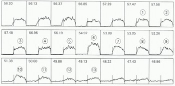
Fig. 7. Reflected radar pulses obtained by the Seasat altimeter as it approached from landward and then crossed the Fimbul ice front.
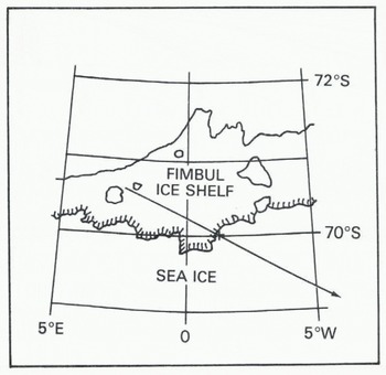
Fig. 8. Seasat orbit 6-209 passing over the Fimbul ice shelf. The cross marks the calculated ice-front position.
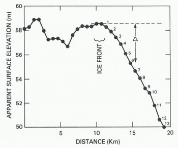
Fig. 9. Apparent surface elevation versus distance along the sub-satellite track for an orbit crossing the Fimbul ice front.
Solution of Equation (2) for the data points (1) to (13) gives a set of circles centered on the corresponding sub-satellite points (Fig.10.). The envelope described by these circles provides a mapping of the ice-front position. In this case, errors in Δ increase as the measurement becomes more oblique and the radar return pulse becomes less distinct. Moreover, there is an additional, unknown error due to variation in ice-shelf height along the ice front. This affects the position of the broken line in Figure 6; each data point (1) to (13) is obtained from portions of ice shelf with different surface elevations. Here, we have tried to assess only the errors associated with the estimation of each range corresponding to frames (1) to (13) in Figure 7 and we have neglected the effects of varying ice-shelf elevation. The corresponding errors in Δ are included in Figure 6, with associated errors fix in calculated distance from sub-satellite point to the ice front. Initially, the errors fix decrease rapidly with increasing distance from the ice front, but then they increase as the radar return pulse becomes less distinct.
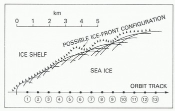
Fig. 10. A portion of the Fimbul ice front derived from radar altimetry measurements.
The presence of icebergs near the coast will contaminate the data to some extent. However, we anticipate that the data may also provide warning of possible iceberg presence, and we are now investigating the prospect of using altimetry data to estimate iceberg concentration.
Summary
Radar-altimetry data from Seasat can be used to map ice-sheet margins with an absolute accuracy of between ±100 m and ±1 km. For an orbit track perpendicular to the ice front, coordinates of the crossing point can be calculated to -±10Q m. However, most orbit tracks crossed the ice front obliquely, providing data from which a 5 to 10 km section of the ice front can be mapped. In these cases, accuracy improves from -±1 km near the crossing point to -±200 m or better for points more than 2 or 3 km away from the crossing point. Seasat crossed the Antarctic coastline at more than 1 000 points, and there are sufficient range measurements to provide high-resolution mapping of almost all of the East Antarctic coastline and the Antarctic Peninsula north of 72°S.
Acknowledgements
This work was supported by the Oceans Program of the National Aeronautic and Space Administration.


