


INTRODUCTION
Satellite observations show numerous regions of strong localized thinning along East Antarctica's Sabrina Coast including the largest outlet of Aurora Basin, Totten Glacier (Pritchard and others, Reference Pritchard, Arthern, Vaughan and Edwards2009; Flament and Rémy, Reference Flament and Rémy2012; Li and others, Reference Li, Rignot, Morlighem, Mouginot and Scheuchl2015). Data from ICESat showed Totten thinning at a rate of 7 m a−1 from 2003 to 2008, which is thought to be driven by contemporary increases in basal melting (Pritchard and others, Reference Pritchard2012). Flament and Rémy (Reference Flament and Rémy2012) analysis of Envisat data showed Totten ice shelf thinning at 1.2 m a−1 from 2002 to 2010. Longer duration data from InSAR (1996–2013) shows thinning of 12 m and retreat of the grounding line by 1–3 km along the east-west trough over 17 a (Li and others, Reference Li, Rignot, Morlighem, Mouginot and Scheuchl2015). Paolo and others (Reference Paolo, Fricker and Padman2015), suggest that satellite radar altimeter data is consistent with Pritchard and others (Reference Pritchard, Arthern, Vaughan and Edwards2009) over the 2003–08 period, but with essentially no change (2.0 ± 7.5 m per decade) over the longer term (1994–2012). Mass-balance calculations based on observed ice thickness and flow speed indicate sub-ice shelf melt rates comparable with the Amundsen Sea Embayment beneath Totten, Dalton and Moscow University ice shelves (Pritchard and others, Reference Pritchard2012; Rignot and others, Reference Rignot, Jacobs, Mouginot and Scheuchl2013), consistent with regional ocean modelling (Gwyther and others, Reference Gwyther, Galton-Fenzi, Hunter and Roberts2014) driven by a warming ocean. Looking to the future, a global ocean model indicates ice shelf basal melting will increase as the Southern Ocean warms in 21st and 22nd centuries (Timmermann and Hellmer, Reference Timmermann and Hellmer2013), and at the same time widespread bedrock lying below sea level and deepening upstream from at least parts of the grounding line means that thinning of ice shelves renders the area potentially unstable through the marine ice-sheet instability (e.g. Moore and others, Reference Moore, Grinsted, Zwinger and Jevrejeva2013). Ice equivalent to ~3.5 m of global sea level is flowing through Totten alone. The larger drainage basin, with a potential contribution of 5.1 m sea level – comparable with West Antarctica ice sheet (Bamber and others, Reference Bamber, Riva, Vermeersen and LeBrocq2009), is grounded below sea level and may become accessible with the retreat of Totten Glacier (Greenbaum and others, Reference Greenbaum2015).
We simulate the evolution of this system in 21st and 22nd century using a time depended ice dynamics model BISICLES, with parameterized sub-ice shelf melting based on ocean models. The sub-ice shelf melting is a simple representation of present day conditions and anomalies caused by ocean warming. This is based on results from a regional ocean model built with the Regional Ocean Modelling System (ROMS) (Shchepetkin and McWilliams, Reference Shchepetkin and McWilliams2005) with modifications for ice shelf/ocean interaction (Dinniman and others, Reference Dinniman, Klinck and Smith2007; Galton-Fenzi and others, Reference Galton-Fenzi, Hunter, Coleman, Marsland and Warner2012). The future anomalies are derived from the Ice2Sea (http://ice2seadata.nerc-bas.ac.uk/thredds/ice2sea/catalogue_ice2sea.html) ocean temperature projections computed with the global ocean model FESOM (Timmermann and others, Reference Timmermann2009), forced in turn by the results from two different climate models, HadCM3 and ECHAM5, that were driven by the ‘business as usual’ IPCC SRES (Special Report on Emissions Scenarios) A1B (Nakicenovic and others, Reference Nakicenovic and Swart2000) and the ‘aggressive mitigation’ E1 (Tol, Reference Tol2006) warming scenarios.
We compare the evolution of Aurora Basin and projected sea level rise (SLR) over the 21st and 22nd centuries under these different warming scenarios and climate models. In addition to dependence on modelled ice shelf basal melt rates and warming scenarios, the choice of ice-sheet basal friction scheme also impacts on ice-sheet evolution in the simulation. We therefore assess simulation sensitivity using both linear and nonlinear forms of Weertman basal friction laws (Weertman, Reference Weertman1957).
MODEL DESCRIPTION
Ice dynamics
We use the BISICLES ice-sheet model in this study (Cornford and others, Reference Cornford2013). The momentum equation is based on the vertically integrated ‘L1L2’ approximation (Schoof and Hindmarsh, Reference Schoof and Hindmarsh2010) and is suited to fast flowing ice streams and ice shelves. Numerically, the model employs a finite volume method with AMR (adaptive mesh refinement), which allows the use of non-uniform, time-dependent meshes. Constructing meshes with coarse resolution in the slowly flowing inland areas and fine meshes around the grounding line and fast flowing areas allows us to capture the behaviour of outlet glaciers without wasting computational resources on the vast inland ice sheet. In this study we implement three refinement levels above the base resolution of 4 km with the mesh gradually refined toward the grounding line, where resolution is 0.5 km (Appendix). Time step varies to satisfy the Courant-Friedrichs-Lewy condition everywhere, meaning ~32 time steps a−1 in Arura Basin. The mesh is updated at each time step.
The 2-D stress-balance equation is
 $$\nabla \cdot \left[{\rm \phi} h{\bar {\rm \mu}} \left(2 {\dot {\epsilon}} + 2tr({\dot {\epsilon}}){\bi I} \right) \right] + {\rm \tau} ^b = {\rm \rho}_igh\nabla s$$
where h is the thickness, $\dot{\epsilon} $
is the strain rate tensor, ρ
i
is the ice density, ϕh is vertically integrated effective viscosity, s is surface elevation and g is gravitational acceleration. We use two formulations for τ
b: linear and nonlinear forms of Weertman friction law in the experiments
$\dot{\epsilon} $
is the strain rate tensor, ρ
i
is the ice density, ϕh is vertically integrated effective viscosity, s is surface elevation and g is gravitational acceleration. We use two formulations for τ
b: linear and nonlinear forms of Weertman friction law in the experiments
 $${\rm \tau} ^{\rm b} = \left\{ {\matrix{ { - C{\left \vert u \right \vert} ^{\left( {\displaystyle{1 \over m} - 1} \right)}u\quad \;if\; \displaystyle{{{\rm \rho}_i} \over {{\rm \rho}_{\rm w}}}h \gt - r} \cr {\quad\quad\enspace 0\quad \quad \ \qquad {\rm otherwise}} \cr}} \right.$$
in which ρ i and ρ w are ice and ocean water density, respectively, r is bed elevation, h is ice thickness, u is horizontal ice velocity and the exponent, m = 1 for the linear friction law and m = 3 for the nonlinear friction law. The friction coefficient C that contributes to basal traction τ b and a stiffening factor ϕ that contributes to the viscosity are calculated by solving an inverse problem, minimizing the difference between modelled velocity and the observed surface velocity (e.g. MacAyeal, Reference MacAyeal1993; Joughin and others, Reference Joughin2009; Morlighem and others, Reference Morlighem2010). The inverse method is described in detail in the study of Cornford and others (Reference Cornford2015).
We carry out each simulation on a 1792 × 1792 km2 domain (Fig. 1) taking bedrock topography and ice thickness at 1 km resolution from Bedmap2 (Fretwell and others, Reference Fretwell2013). The sea bed topography data beneath the Totten and Dalton ice shelves is poorly constrained in Bedmap2. We therefore modify the bathymetry following Gwyther and others (Reference Gwyther, Galton-Fenzi, Hunter and Roberts2014). This means we deepen the cavity by a depth R C. According to Greenbaum and others (Reference Greenbaum2015), it is an average of 500 m deeper along the long axis of Totten cavity. So instead of setting R C = 300 m as Gwyther and others (Reference Gwyther, Galton-Fenzi, Hunter and Roberts2014), we set R C = 500 m along the cavity centreline, while along the grounding line, R C = 0. Within the cavity, R C is linearly interpolated between the cavity centreline and grounding line. In this study, parameterized melt rate depends only upon the depth of ice shelf bottom, so R C will not affect the sub-ice shelf melt, but deepening the sea bed removes some very thin cavities beneath the ice shelf that would otherwise lead to immediate grounding. The 3-D temperature field used in the simulations is taken from Pattyn (Reference Pattyn2010) and is fixed over time. The surface mass-balance field is taken from Arthern and others (Reference Arthern, Winebrenner and Vaughan2006). The calving front is fixed in this study. Finally, the basal traction and stiffening factor are determined from surface velocity data (Rignot and others, Reference Rignot, Mouginot and Scheuchl2011) with one notable exception: there is no data in the eastern part of Law Dome, so we set the basal traction coefficient there to the similar value as in the western half so that the bedrock elevation and surface slopes are similar (Fig. 2b).
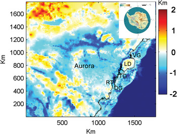
Fig. 1. The simulation region with bed elevation (colour bar) showing Totten Glacier (TG), Dalton Glacier (DG), Vanderford Glacier (VG), Law Dome (LD) and Reynolds Trough (RT). The insert shows a map of Antarctica with the study region outlined in black.

Fig. 2. The initial conditions for experiments after 50 a of surface relaxation around Totten, Dalton and Vanderford glaciers, (a) μe is the effective viscosity coefficient, (b) βe is the logarithm of basal friction coefficient log10 C, (c) M
0 is the initial ice shelf basal melt rate, (d) $\left \vert\vec u\right \vert$
is the magnitude of surface velocity.
$\left \vert\vec u\right \vert$
is the magnitude of surface velocity.
We find high-amplitude short-wavelength thickening or thinning at the initial stage of simulation. It presents a strong signal of change early in a simulation that results from non-physical causes and can mask the response to future climate anomalies. The magnitude of fluctuations is as large as 300 m a−1 in places. We assume this unrealistic behaviour is due to discrepancy between the initial thickness and velocity, caused by the different epochs for measurements of geometry and ice velocity, interpolation method or undersampling. We attempt to address this issue by relaxing the geometry (Gong and others, Reference Gong, Cornford and Payne2014; Wright and others, Reference Wright2014). After 15 a almost all the grounded ice has thickness changes <10 m a−1, and the grounding line has stabilized, and the ice thickness differs from bedmap2 by <100 m. A major exception is the southern flank of Totten glacier, which thins throughout the relaxation and indeed through every subsequent experiment. The bedrock in this region is only sparsely covered by airborne radar (Fretwell and others, Reference Fretwell2013), and so we assume the initial ice thickness is incorrect. The knock-on effect on other parts of the basin appears to be small – for example, as we will show, retreat along the trough between the Totten and Vanderford glaciers is conditional on the future ocean forcing, and does not take place without elevated melt rates. In common with Cornford and others (Reference Cornford2015) and Gong and others (Reference Gong, Cornford and Payne2014), we begin simulations with variable forcing after 50 a of relaxation with present-day climate, by which time the mean thickness change in the domain is 2.4 m.
Melt-rate parameterizations
Climate forcing from atmosphere and ocean impact ice-sheet dynamics by surface snow accumulation and sub-ice shelf melt, and the ice-sheet model responds to the two perturbations independently (Cornford and others, Reference Cornford2015). Dynamical thinning is the major mechanism by which mass is lost, and that is projected to be primarily forced by changes in the ocean for the next 2 centuries. So, in this study we keep the surface mass balance constant and consider only variation in the ice shelf basal melt rate. The ‘melt rate’ refers to ‘ice shelf basal melt rate’, and upper surface melt rates are not discussed further in the current study.
Sub-ice shelf melt rate is influenced by ocean conditions and the ice draft. Ideally, the simulation of melt rate would be carried out within a coupled ocean/ice shelf/ice-sheet model, but lacking such a model we examine the response of the ice-sheet model to simple melt-rate formulae constructed in light of the results of standalone ocean models. Each melt-rate formula is composed from a depth-dependent part based on a model of the present day, denoted by M, and a time-dependent part derived from emission driven climate projections, denoted by M a.
Present-day melt rates are parameterized based on an ocean model of the Totten ice shelf region (Gwyther and others, Reference Gwyther, Galton-Fenzi, Hunter and Roberts2014), which was re-run with forcing conditions updated to cover the 1992–2012 period. The time-averaged melt rates are consistent with a parameterization of the melt rate as a function of ice shelf thickness. Figure 3a shows the fit between the parameterized melt rate and the modelled melt rate. Figure 2 shows the reconstructed melt rate based on the average modelled melt rates between 1992 and 2012 in the Aurora coastal area. We parameterize this data with a simple, depth dependent formulation (Asay-Davis and others, Reference Asay-Davis2015):
 $$M = Ad(T - T_{\rm f})\tanh \left( {\displaystyle{w \over {H_{\rm c}}}} \right),$$
where d is the depth of ice shelf bottom, T f is the freezing point. T is the far field ocean temperature. w is the thickness of water column beneath ice shelf. H c = 75.0 m is the reference ocean cavity thickness. A satisfactory fit for (3) is found setting T = −1.5°C, and A = −7.4 × 10⁻⁷ a−1°C−1, of which RMSE between the parameterized and mean melt rate is 3.8 m a−1 (Fig. 3). In a previous study the parameterisation method is calibrated using the POP ocean model with idealized geometry (Asay-Davis and others, Reference Asay-Davis2015). However, the melt-rate parameterisation does not include ice/ocean interface slope, or any changes in hydrography resulting from external forcing, such as climate change. Therefore parameters used in this study are not likely to be appropriate for other ice shelves, or even this ice shelf for long duration simulations. Figure 3 shows the spatial variability of melt rates (blue dots). The parameterized melt rate (black line) fits the mean melt rates (red dots) of ice shelf thickness, this implies the parameterization will not well capture 2-D variability in melt rates. Considering that the highest melt rate is around the grounding line, which is important to ice dynamics and might be underestimated here, we also consider an experiment with higher melt-rate anomaly.

Fig. 3. Parameterization of melt rate. (a) Simulated average melt 1980–2012 from ROMS and its parameterization (Eqn. (3)) as a function of ice shelf thickness. Mean melt rate at a given thickness is the average over all grid cells where the ice thickness is between thickness −Δd and thickness +Δd. 210 values of thickness between 86 m and 2644 m are taken. (b) Time evolution of melt rate anomalies produced by temperature anomalies from FESOM $(M_{\rm a} = 16{\rm \; m\;} {\rm a}^{ - 1}{\rm ^\circ} {\rm C}^{ - 1} \times \Delta T)$
driven by different climate models under different scenarios and the parameterization of Eqns (4) and (5).
$(M_{\rm a} = 16{\rm \; m\;} {\rm a}^{ - 1}{\rm ^\circ} {\rm C}^{ - 1} \times \Delta T)$
driven by different climate models under different scenarios and the parameterization of Eqns (4) and (5).
Future anomalies are derived from the Ice2Sea FESOM simulations (Timmermann and others, Reference Timmermann2009; Timmermann and Hellmer, Reference Timmermann and Hellmer2013), which were driven by the two global climate models (with 1.25°–1.5° resolution for the ocean): HadCM3 and ECHAM5 in turn driven by two emissions scenarios: A1B and E1. Projections span 1980–2100 for ECHAM5 under both A1B and E1, 1980–2150 for HadCM3 under E1, and 1980–2200 for HadCM3 under A1B. FESOM is not able to resolve the small ice shelves along the Sabrina Coast, much as it could not resolve the Amundsen Sea ice shelves, as pointed out in Cornford and others (Reference Cornford2015). So rather than employ FESOM melt-rate anomalies directly we follow Cornford and others (Reference Cornford2015), who assumed a simple relationship between temperature anomalies ΔT in the nearby ocean and melt-rate anomalies M a = 16 m a−1°C−1 × ΔT at the upper end of the range of observations and model studies (Rignot and others, Reference Rignot2002; Holland and others, Reference Holland, Jenkins and Holland2008). This linear relationship between melt-rate anomaly and ΔT might cause some errors especially when the warming trend is significant. Holland and others (Reference Holland, Jenkins and Holland2008) pointed out that, for ice shelf with high melt rate, the relationship between melt rate and thermal driving is nonlinear. Ocean temperature is characterized by averaging FESOM temperatures over a volume bounded laterally between the present day ice front, the 1000 m ocean depth contour and the extreme longitudes of the Aurora Basin and vertically between 200 and 800 m below sea level. This volume samples water masses that can both cross the continental shelf and access most of the sub-ice shelf cavity. FESOM temperatures differ considerably between the two climate models, but for each model, independent of climate scenarios. When driven by HadCM3, FESOM temperature rise 1°C by 2150 then remain almost constant, while under ECHAM5 they steadily decrease. Therefore we parameterize melt-rate anomalies over time as:
 $$M_{\rm a} = \left\{ {\matrix{ {7.2 \times {10}^{ - 4}t^2 - 0.027t + 0.7\; \; {\rm m}\; \,{\rm a}^{ - 1},} & {\; t \le 170\; \,{\rm a}} \cr {16\; \,{\rm m}\,{\rm a}^{ - 1},} & {{\rm otherwise}} \cr}} \right.,$$
for HadCM3, and
 $$M_{\rm a} = - 0.01t - 0.2\; {\rm m\;} {\rm a}^{ - 1},$$
for ECHAM5, where t is the time in years since 1980 in Eqns (4) and (5) (Fig. 3b). Figure 3b shows the fit of parameterized melt rate (lines) to melt rates calculated based on temperature anomalies produces by FESOM ocean model (scatters). The RMSE for ECHAM5 is 0.4 m a−1 under the E1 scenario and 0.6 m a−1 under the A1B scenario. The RMSE for HadCM3 is 1.3 m a−1 for E1 scenario and 1.2 m a−1 under the A1B scenario. There are significant differences between the projections from HadCM3 and ECHAM5. There are number of ways such differences can propagate through the regional ocean to the ice shelf. Higher air temperature over the southern ocean or higher ocean temperature at the FESOM northern boundary could cause universally higher temperatures in FESOM, causing increased shelf melting. Changes in prevailing wind over the southern ocean could potentially re-route water masses, affecting whether or not warmer water masses (such as CDW) come in contact with the ice shelf. Difference in sea ice extents and concentrations could greatly affect the air/sea exchange of heat and therefore water temperature. In the current study, the difference in the temperature anomaly simulated by FESOM forced by HadCM3 versus ECHAM5 results from the different surface heat flux simulated by each GCM (Timmermann and Hellmer, Reference Timmermann and Hellmer2013).
We carry out a total of seven experiments, summarized in Table 1. Two (Ctrl/m1 and Ctrl/m3) are forced for 200 a by applying the present day melt rate (3) with M a = 0 to BISICLES model with the linear and nonlinear Weertman basal friction laws. Two (Had/m1 and Had/m3) come from applying the HadCM3 anomaly (4) to BISICLES model with the linear and nonlinear Weertman basal friction laws. A fifth (EC5/m1) applies the ECHAM5 anomaly to a BISICLES model with the linear basal friction law, a sixth (2 × Had/ml) doubles the melt rate of Had/m1, and the seventh (ka Had/m1) extends the Had/m1 simulation to t = ka.
Table 1. Experiment settings used

RESULTS
Sensitivity to ice shelf melting
Linear basal friction
The grounding lines of both Dalton glacier and Totten glacier retreat over the coming centuries under each of the climate forcings (Fig. 4). The grounding line of Vanderford glacier retreats provided that melt rates are at least as high as those driven by HadCM3 (Fig. 4).

Fig. 4. Grounding line location (coloured lines – see legend for experiment) at the end of the different simulation experiments (Table 1). Colour bar is bed elevation above sea level.
For the Totten glacier, the grounding line retreats west along the trough adjacent to Law Dome in some cases and east toward Dalton ice shelf in general. Retreat along the deep trough, where present day melt rates are highest, only takes place when melt rates are at least as large as those driven by HadCM3 (Had/m1, 2 × Had/m1), and after ice shelves of Totten and Vanderford glaciers are merged, the grounding line will not retreat further inland. Nonetheless, doubling the melt rate doubles the rate of retreat from 10 km over 200 a in the Had/m1 experiment to 20 km in the 2 × Had/m1 case. The southern flank and eastern end of the ice shelf retreat in every experiment, but the larger HadCM3 melt rates are required to drive the grounding line across a shallow area between the Totten and Dalton ice shelves.
The grounding line of Dalton glacier retreats gradually along the Reynolds trough to the west until the grounding line reaches the end of the trough. Once again, the higher the melt rate, the faster the grounding line retreats, with the ECHAM5 forcing producing 25 km retreat over 200 a, present day forcing producing 50 km, and the HadCM3 forcing producing 75 km. However, additional forcing has no effect: grounding line locations are nearly the same at the end of the 22nd century when forced by HadCM3 as when forced by twice that melt rate, having reached a region of pro-grade south-facing slopes.
Vanderford Glacier appears to exhibit a rather straightforward marine ice-sheet instability. Its present day grounding line is located on a ridge, and the stronger HadCM3 melt rates are needed to drive it toward the deeper beds inland. Provided that the grounding line does enter the region with deeper bedded, it retreats for 100 km in an easterly direction along the trough within 200 a under HadCM3 forcing and a further 50 km when the melt rates are doubled, in which case it is close to joining with Totten Glacier's grounding line.
The ka simulation sees the grounding line reach a stable location after some hundreds of years, located on bedrock sloping downward to the sea. The deep trough between the continent and Law Dome is occupied by floating ice, so Law Dome is separated from the main continental part of Aurora Basin.
The change of ice volume above floatation is a measure of ice-sheet contribution to global sea level, so we calculate the anomaly of ice volume above floatation (VAF) relative to present day in the model domain (Fig. 5a). Although grounding lines retreat in all experiments, VAF increases when the ice sheet is forced by melt rates generated using ECHAM5 climate model output (simulation EC5/m1). VAF decreases in all the other simulations, and higher melt rate leads to larger contributions to SLR.

Fig. 5. (a) Change in volume above floatation (VAF) of the Aurora Basin relative to present day. (b) SLR contribution of the Aurora Basin.
The contribution of Aurora Basin to the rate of SLR is shown in Figure 5b. For the control experiment and the experiment with negative melt anomaly calculated using ECHAM5 output, the annual contribution to SLR has a decreasing trend, from ~0.1 mm a−1 to zero or even slightly negative. For simulations with higher melt rate anomalies, SLR contribution increases during the first century, and decreases from around the year 2150 to ~0.1 mm a−1 at the end of the 22nd century.
Nonlinear basal friction
Rates of grounding line movement are only modestly sensitive to the choice of basal friction law. Using the nonlinear basal friction law without additional forcing (Fig. 4, Ctrl/m3) results in the grounding line retreating ~8 km further compared with the linear basal friction law (Fig. 4, Ctrl/m1) on the eastern part of Totten glacier adjacent to the Aurora continental coast and along the Reynolds trough. Similarly, the experiment forced by HadCM3 with a nonlinear friction law (Fig. 4, Had/m3) causes ~10 km more retreat of the grounding line than with a linear friction law (Fig. 4, Had/m1) in Vanderford glacier. Overall, the grounding line positions for m = 3 lies close to their m = 1 counterparts compared with the difference due to increases in the melt rate.
Unlike grounding line retreat, the total discharge is sensitive to the choice of friction law (Fig. 5). Without melt rate anomalies there are 3 × 10³ km3 extra contribution to SLR from nonlinear Weertman sliding compared with the same case with linear Weertman sliding, and 7.5 × 10³ km3 when forced by melt rate calculated using HadCM3 forcing. In fact the loss of VAF using the nonlinear friction law and forced by HadCM3 exceeds that when using the linear friction law and doubled melt rate. At the same time annual SLR contribution has less interannual variability with nonlinear friction law and increases faster.
Climate model and scenario
Melt rates anomaly difference due to different climate scenarios is pretty small compared with that between different climate models. HadCM3-forced simulations are generally warmer than ECHAM5-forced simulations, which display a consistent cold bias and a surface salt bias (Timmermann and Hellmer, Reference Timmermann and Hellmer2013). This is due to larger surface heat loss over the Antarctic continental shelf in ECHAM5, which drives stronger ice production, cooling and salinification bias (Timmermann and Hellmer, Reference Timmermann and Hellmer2013). There are enormous differences in the evolution of melt rates between the FESOM's temperature response to the two forcings, from which we produce an enormous difference in melt rates. ECHAM5 driven forcing predicts a slight decrease in melt rates, while HadCM3 forcing leads to increasing melt rates over the simulation period. Hence conclusions on the fate of the ice shelf are entirely climate model dependent and – from these two models – appears to be independent of emissions scenario. This is counter-intuitive and strongly suggests that at least one of the model climates around the Aurora Basin region is simply wrong under both sets of emissions. Whether this is a result of inadequate model physics or lack of resolution is beyond the scope of this paper. The issue may be resolved using a larger climate model ensemble, or by global models that prioritize simulation of Southern Ocean climate. It is not possible to say, which model is producing more reasonable future ocean temperatures since it is highly likely that greenhouse gas forcing lowers the strength of the global thermohaline circulation (Cheng and others, Reference Cheng, Chiang and Zhang2013), which may lead to cooling of some regions. The simulation of Antarctic sea ice is also critical to the correct calculation of ocean circulation as is atmospheric circulation and its influence of warm ocean water up-welling (Pritchard and others, Reference Pritchard2012; McCusker and others, Reference McCusker, Battisti and Bitz2015).
DISCUSSION
In this section, we discuss the evolution of the Aurora Basins major outlets: Totten, Dalton and Vanderford glaciers, over the 21st century and 22nd century, and the impact of ocean warming and basal friction to this evolution. The limitations of our method are also discussed.
Ice mass loss of Aurora basin is sensitive to ice shelves thinning by ocean warming. The ice-sheet model produces 6000–14 000 km3 loss of ice or a SLR of 15–35 mm over 2 centuries. This is about half the mass loss from West Antarctica when forced by temperature anomalies produced by the FESOM ocean model (Cornford and others, Reference Cornford2015). The basin is potentially unstable under ocean warming. However, in our simulation, the influence of ocean warming to ice-sheet retreat would be limited to ~3 centuries in our experiment; grounding line retreat and ice mass loss stop after that (Fig. 4).
Bedrock topography plays a major role in the evolution of this region of the East Antarctic ice sheet. Grounding lines retreat along the deep troughs with either present day melt rate or lower (as found when driven by the ECHAM5 climate model) for both Dalton and Totten ice shelves. Recent research also suggests that ocean warming contributes to the retreat of the eastern Totten glacier grounding zone and may contribute to further destabilization of low-lying area between Totten glacier and the Reynolds trough (Sun and others, Reference Sun, Cornford, Liu and Moore2014; Greenbaum and others, Reference Greenbaum2015). We show this potential instability and the accelerating effect of ocean warming in our simulations. Most of the grounding line retreat we do simulate is along bedrock troughs parallel to the coast, while retreat toward the south tends to be limited due to the pro-grade slope running from north-to-south (e.g. Schoof, Reference Schoof2007).
Although grounding line retreat occurs in every simulation, VAF can be stable or slightly increase when forced by melt rates slightly lower than present day ones, because ice accumulation in the inland ice sheet then offsets the mass lost in the coastal region.
Basal friction, and in particular the form of the relationship between friction and velocity is an important control. Given the same melt rates, grounding lines retreat only a little further when the nonlinear friction law is chosen (Had/m3) compared with the linear friction law (Had/m1) but lose more than twice the VAF; given similar VAF loss (2 × Had/m1 compared with Had/m3) grounding line retreat is far lower. This apparently paradoxical outcome is in fact straightforward to explain: given larger m (Eqn. (2)), we get larger basal friction factor C everywhere of the whole basin. When the ice shelf is thinning, ice flow speeds up more to balance the loss of buttressing with larger m (Eqn. (1)), so the grounding line retreats further and more VAF is lost. Since the acceleration and thinning occurs over the whole region, a modest grounding line retreat is combined with large VAF loses for the whole basin.
In summary, ocean warming can accelerate the ice-sheet retreat in Aurora Basin. However one climate model we use suggested little or no warming around the Aurora Basin at depths suitable for ice shelf melting to increase, while the other model leads to considerably increased melting. Bedrock topography controls the stability of ice sheet, so recent surveys to improve the quality of bedrock elevation data should provide valuable information. More precise bathymetry data is the most useful for improved simulation of the region. Similarly, the lack of accurate ice velocities, which may be improved by further observations, leads to an assumed basal friction being applied to part of Law Dome. The basal sliding scheme is also an essential boundary condition, which impacts the ice-sheet acceleration rate and its contribution to SLR. Improved understanding and parameterization of basal processes, such as resulting from new model inter-comparison experiments, will also be valuable.
There are some potentially serious limitations of our methods. We do not include the calving event in our simulation. Ice shelf buttressing effect is decreased by both thinning and calving. Recent study (Fürst and others, Reference Fürst2016) suggests that the area of ‘passive ice’ for Totten glacier is relatively small (4.2%), which means even a small loss of ice from calving front would cause changes in flux across the grounding line. Since some observation data and ocean model results show a thinning trend for Totten ice shelf, which would impact the calving process, further investigation of buttressing field changes under present day and future ocean conditions is merited. In the parameterization of present day melt rate, we take the mean melt rate as a function of ice thickness, which does not account for 3-D variability as may be expected to arise because of potential change in sub-ice shelf ocean currents as the cavity geometry evolves, or the impacts of varying sub-glacial water discharge across the grounding line. The highest present-day melt rate in our simulation is <50 m a−1, as this is a depth-binned average, while the value in ROMS output is 80 m a−1, illustrating the possible range of errors simply due to parameterization errors. In the parameterization of future melt rate anomalies, we treat melt rate as a linear function of ΔT and simulate it as constant over space. This is unlikely to be true, with variability expected over both time and space as the ice shelf cavity evolves, and also as the global climate, ocean circulation, sea ice cover and wind stress fields evolve. Some improvements in model may be possible by parameterizing melt anomaly in terms of more sophisticated geometry. While we have demonstrated the sensitivity of the Aurora basin to ice shelf melting, we have not established likely future ice shelf melt predictions for any given emissions scenario, due to the wide discrepancy between. This suggests that closer inspection of the Southern Ocean processes such as atmospheric circulation-driven warm water upwelling, and sea/ice interactions with changed radiative forcing and their implementation in climate models, may be fruitful.
ACKNOWLEDGEMENTS
This study is supported by China Postdoctoral Science Foundation NO. 212400240; the National Natural Science Foundation of China (41506212); National Key Science Program for Global Change Research NO. 2012|CB957702, 2015CB953601 and 2015CB953602. BISICLES development is with financial support provided by the US Department of Energy and the UK Natural Environment Research Council.
APPENDIX
MESH SENSITIVITY
Before making sensitivity experiments, we must choose a suitable mesh since the simulation of the grounding line region is sensitive to resolution (Vieli and Payne, Reference Vieli and Payne2005). In this section, we demonstrate that our 3 level refinement mesh, with the finest resolution 0.5 km, is appropriate.
Figure 6 show the grounding line position at the end of 22nd century of experiments with linear friction law and melt rate forced by HadCM3 carried out on a sequence of meshes with the finest resolution Δx = 4, 2, 1, 0.5 and 0.25 km. The differences between the coarsest mesh and other finer meshes are evident on all ice shelves. The coarse mesh simulation cannot show the active retreating on the southern of Totten ice shelf, and the grounding line retreat of Dalton is ~30 km less than other finer mesh results. Both Δx = 4 km and Δx = 2 km resolution cannot show the grounding line retreat of Vanderford glacier, and the retreat in Δx = 1 km is ~30 km less than the sub-kilometre experiments. The behaviours of ice shelves are quite similar for Δx = 0.5 km and Δx = 0.25 km resolution experiments.

Fig. 6. Grounding line locations in year 2200 under different levels of mesh refinement.
Considering the performance of ice-sheet model and also the consuming of computational resources, we chose the 3 level mesh with Δx = 0.5 km.


 Open access