


Introduction
The remote, harsh environments of Greenland and Antarctica make in situ collection of ice-velocity and elevation data difficult. Great expense and human effort has gone into the field measurements that have been made. Over the last decade, satellite remote sensing has developed to a point where it is now possible to make accurate, high-resolution measurements of many ice-sheet parameters. Radar altimeters, for example, have provided elevation models over all of Greenland and much of Antarctica (Reference Bamber, Ekholm and KrabillBamber and others, 1997). Introduced recently, satellite radar interferometry (Reference Goldstein, Engelhardt, Kamb and FrolichGoldstein and others, 1993) has emerged as a powerful method for measuring ice-flow velocity and surface topography.
For the most part, spaceborne observations are limited to the surface of the ice sheet. Yet many of the controls on ice flow manifest themselves below the surface. Inversions of ice-sheet models constrained by remotely sensed data have been used to help explain internal dynamic processes of ice flow (Reference MacAyeal, Bindschadler and ScambosMacAyeal and others, 1995). These have yielded promising results, but the development and further application of such inverse techniques has been limited by a scarcity of data. Satellite radar interferometry now provides a means to begin filling this data gap.
We have begun an investigation that uses a combination of remote-sensing and modeling techniques to study the northeast Greenland ice stream. This ice stream was first recognized in satellite imagery, where it appears as a nearly straight feature about 700 km long with identifiable margins for most of its length and a topographically undulating interior resulting from rapid ice flow over the bed topography (Reference Fahnestock, Bindschadler, Kwok and JezekFahnestock and others, 1993). The organized flow extends far into the interior, beginning within about 100 km of the ice divide. Near the coast it has low-slope areas of rapid flow and regions of enhanced shear that resemble the West Antarctic ice streams.
This paper describes the remote-sensing component of our investigation. We present a vector velocity map that covers the entire ice stream. We describe the map generation and validate our results through a comparison with independent global positioning system (GPS) measurements. Finally, we describe the use of interferometric techniques to improve the resolution of a digital elevation model (DEM) for the ice stream that was originally derived primarily from radar altimetry data.
Velocity Field
Figure 1 shows the final product, a velocity map, that we have derived for the northeast Greenland ice stream using interferometric data from several ascending and descending European remote-sensing satellite (ERS) orbits. These data were collected during the commissioning and ice orbital phases of ERS-1 as well as the ERS-1/-2 tandem mission.
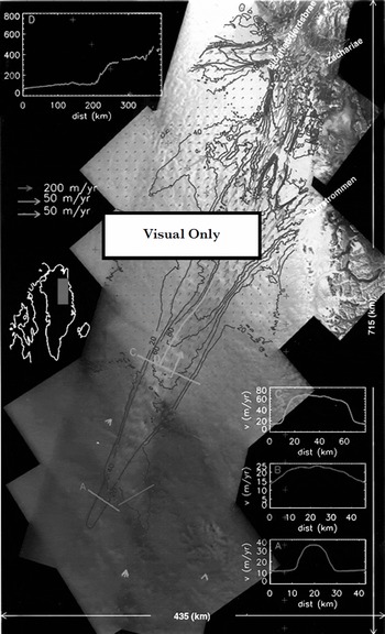
Fig. 1. Velocity map for the northeast Greenland ice stream. Green contours at 20 m a’1 intervals are used for speeds up to 80 m a–1; blue contours at l00 m a–1 are used for6 higher –speeds.RedarroWsshoWvelocity.SPeedisplottedalonga A-Care straight lines across the ice stream, while D corresponds to a flowline along the ice stream. Red crosses mark the locations of GPS-derived velocities. GPS velocities used for validation are illustrated with yellow vectors, and cyan vectors are used for corresponding interferometric measurements. SAP imagery copyright European Space Agency 1999.
The velocity map confirms that the ice stream begins as a narrow (10–15 km) band of enhanced flow. Although the flow is not exceptionally fast at this point (15–30 m a"1), it is much faster than that of the surrounding ice, with well-defined shear margins (see profile A, Fig. 1). Further downstream a tributary of enhanced flow merges with the ice stream. This is much broader and, in contrast to the first tributary, lacks well-defined shear margins (see profile B, Fig. 1).
Roughly 100 km downstream, the ice stream broadens out to a width of nearly 50 km with speeds of 50–75 ma"1 (profile C Fig. 1). From here, the speed increases gradually downstream over the next 200 km until increasing abruptly from roughly 100 m a to 300–400 m a–1 over a distance of approximately 20 km (profile D, Fig. 1). This increase in speed coincides with a peak and then rapid decline in the driving stress, which is similar to that observed for ice-stream onsets in West Antarctica (Reference BentleyBentley, 1987). The flow then divides to contribute ice to three major outlet glaciers: Nioghalvfjerdsbræ, Zachariæ, and Storstrommen. The data also show that Nioghalvfjerdsbræ derives much of its ice from an independent tributary.
Interferometric control
Interferometric estimates of ice velocity require cm-level accuracies for the interferometer baseline Reference Joughin, Kwok and FahnestockJoughin and others, 1996a). Baselines determined from the precision orbital-state vectors for the ERS satellites do not provide sufficient baseline accuracy for most glaciological applications. Instead, elevation and velocity control points are needed to solve for the baseline.
For regions near the coast, areas of exposed bedrock can be used for control, reducing the need for velocity measurements (Reference Joughin, Kwok and FahnestockJoughin and others, 1996a). Many of the scenes we used, however, were well away from the coast, so there was little or no ice-free area to provide a source of control.
We originally intended to use GPS-surveyed velocities (personal communication from R. H. Thomas, 1998) as control points. These surveys were collected by the NASA Program for Arctic Regional Climate Assessment (PARCA) along the 2000 m contour of Greenland to calculate ice-sheet discharge (Reference Thomas, Csatho, Gogineni, Jezek and KuivinenThomas and others, 1998). Additional data were collected as part of this effort near the onset area of the ice stream, specifically for use as interferometric control points. The points used in our study are indicated with red crosses in Figure 1. Unfortunately, there were not enough points to provide control for all of the interferometric swaths. Furthermore, in swaths where we did have at least the necessary minimum of four points, interferometric phase errors were often so large that we could not achieve the desired baseline accuracy. Because we use a least-squares fit to the control points to determine the baseline parameters, it is possible to mitigate the effects of phase noise by using more control points.
With an insufficient number of GPS control points, we opted to use balance velocities as a source of control. Balance velocities are the depth-averaged velocities necessary to maintain the steady-state shape of the ice sheet and are estimated from surface slope, ice thickness and accumulation data (Reference PatersonPaterson, 1994). We computed these values as described by Reference Joughin, Fahnestock, Ekholm and KwokJoughin and others (1997) and rescaled them by a factor of 1.1 to obtain surface-velocity estimates. Better estimates of the spatially variable conversion factor from depth-averaged to surface velocity could be obtained with a thermomechanical ice-sheet model (Reference Thomas, Csatho, Gogineni, Jezek and KuivinenThomas and others, 1998). The effect on the surface velocities determined from balance velocities, however, would be small (a few per cent) with respect to other sources of error.
Errors in the source data (e.g. accumulation, thickness) can lead to large errors in the balance-velocity estimates. To minimize the impact of balance-velocity errors on our baseline estimates, we selected control points in slow-moving areas outside of the ice stream, where the absolute errors in the balance velocities are small. For example, if the velocity is 10 m a"1, then even a large relative error of 50% leads to an absolute error of only 5 ma–1. Thus, by selecting balance velocities from slow-moving areas we are able to provide a reasonable constraint for the fast-moving ice in the ice stream. Furthermore, since flow in the slow-moving areas should be governed by sheet flow, we select control points from the most dynamically stable area and the area that, barring large changes in accumulation/ablation patterns, is least likely to be out of balance given the long dynamic response time of the Greenland ice sheet (Reference PatersonPaterson, 1994).
To keep absolute errors small, we used only control points where the balance velocity was ω40 m a"1. There are 26 GPS points from the area shown in Figure 1 that meet this criterion, allowing us to quantify the balance-velocity error. If we assume zero error in the GPS estimates, vGPS, then the root-mean-square (rms) error for the balance velocities, vb,6 is givεn by
where the × and y directions are defined by the polar stereographic projection (a; directed south along –45° longitude, y along –135°). Using this metric, the error for the 26 points is 5.5 m a"1. For many of the interior strips, we were able to set a much lower threshold for the balance velocities. For an upper limit of 10 m a"1, the rms error drops to 2.4 m a–1 for the 12 GPS points that he below this threshold.
The comparison with GPS data indicates that the balance velocities provide a reasonable source of control. With the ability to use several dozen points in each baseline solution, we are able to greatly reduce the effects of interferometric phase noise on the baseline solution. In addition, the large number of points helps mitigate the effect of the random component of the control-point noise. This does little, however, to reduce the effect of systematic trends in the control-point data (i.e. a linear error in the balance velocities across a scene).
The elevation at the control points is required for baseline estimates. On the ice, the elevation-control data we used were extracted from a DEM derived primarily from radar altimetry (Reference Bamber, Ekholm and KrabillBamber and others, 1997). Additional data from ice-free areas were derived from a DEM produced by the Danish National Survey and Cadastre (Reference EkholmEkholm, 1996).
Velocity map generation
To create the map (Fig. 1), we began by solving for the baseline for each swath. For the ascending swaths we relied entirely on balance velocities and ice-free points near the coast. For the descending data we first determined the baselines for the inland descending swaths using balance velocities. We then produced a map of velocity for the inland areas. Next, we used data from the faster-moving points of this initial map to provide a source of control for the descending swaths nearer the coast. By bootstrapping in this manner, we were able to avoid the direct use of balance velocities for some of the swaths with predominantly fast motion.
The technique we used to make velocity measurements for individual scenes has been described elsewhere Reference Joughin, Kwok and FahnestockJoughin and others, 1996a, Reference Joughin, Kwok and Fahnestock1998). Unlike our earlier maps, this map involved combining many swaths of crossing ascending and descending orbits (17 swaths of data). The intersections of pairs of crossing orbits produce small patches that must be mosaicked together to create the overall map. These small patches are generally much more numerous than the synthetic-aperture radar (SAR) swaths.
In the mosaicking process for each ascending image, we looped through the descending images to find the areas of overlap over which to estimate the velocity. To avoid discontinuities, we weighted the edges of each patch with a linear taper. While this ˚feathering" operation does not improve accuracy, it does minimize small discontinuities that would otherwise be present in the data. Such discontinuities are non-physical and can lead to problems when attempting model inversions. Next, the data were weighted to reflect the errors (as described below) and summed in an output buffer. The weighting factor, which includes the taper, was tracked in a separate buffer for each horizontal component. Once all the data had been summed, they were normalized using the accumulated weights to compute the weighted average.
We used data with a variety of temporal baselines. With the tandem data we could use 1, 35 and 36 day temporal baselines. The ERS-1 Commissioning and Ice phases yielded temporal baselines of 3, 6 and 9 days. The dominant noise sources in our data are atmospheric and other phase artifacts not related to interferometric decorrelation. These errors are, for the most part, independent of the temporal separation. Thus, with longer intervals between SAR observations a larger displacement signal is observed relative to the fixed level of error. As a result, we assume that the temporal separation is inversely proportional to the velocity error, which provides us with an estimate of the relative variances for the velocity errors.
Velocity estimates from a pair of overlapping ascending and descending interferograms may have different temporal baselines. Consequently, we estimate the phase variance for each interferogram separately and apply the appropriate rotation to derive the individual variance estimates for each component of velocity. The weighting factors used for each component are then inversely proportional to the variance.
Comparison with GPS
The control for the velocity map, even with the bootstrapping described above, was based entirely on balance velocities and ice-free points near the coast. We did not use the GPS velocities to create the map. Instead, we held these points back for use in validating our results. There were 12 GPS points within the area mapped. These velocities are plotted as yellow vectors in Figure 1. For comparison we have included the corresponding interferometric estimates plotted as cyan vectors.
The rms error for the interferometric estimates given by Equation (1) is 5.0 ma–1. Table 1 gives the mean and rms errors for the individual components and speed. The rms error in the y direction, 4.7 m a"1, is ≥ 2.5 times that in the × direction. The smaller error in the × component likely reflects the fact that many of the descending swaths, which are more sensitive to the × component of velocity, have a temporal baseline of 35 or 36 days, while none of the ascending data had a temporal baseline of ≥ 9 days.
Table 1. Mean and rms difference between interferometric and GPS velocity estimates
The largest errors tended to occur among the seven points that followed the NASA PARCA Greenland traverse. As indicated above, the control points in these faster-moving regions are subject to larger errors, which may in part explain the larger errors we observed.
Two of the largest errors occur near the junction where the flow divides to feed Storstrommen and Zachariæ/Nioghalv-fierdsbne. The dominant interferometric data in this region were collected with 6 day intervals in January and February 1994. With a relatively long temporal baseline of 6 days, the error should be relatively small in this region. Thus, we find it surprising that the largest errors were found here.
Storstrommen surged during the period 1978–84 (Reference Reeh, Boggild and OerterReeh and others, 1994). Reference Mohr, Reeh and MadsenMohr and others (1998) mapped the stagnant front of Storstrommen interferometrically with ERS data acquired in 1995, concluding that the glacier is in the process of returning to its pre-surge state. Thus, at least in its lower reaches, Storstrommen is experiencing changes in its pattern of flow. Further inland, the NASA PARCA GPS velocity data were derived from displacements measured from surveyed pole locations in May 1996 and in May 1997, roughly 2.5 years after the interferometric data were collected. Therefore, it is possible that the large difference for these two points during this period might be explained by changes in the relative discharge between post-surge Storstrommen and Zachariæ/Nioghalvfjerdsbne.
DEM
As well as providing velocity information, satellite radar interferometry can be used to estimate ice-sheet elevation with a resolution of 100 m or better (Reference Joughin, Winebrenner, Fahnestock, Kwok and KrabillJoughin and others, 1996b). In contrast, radar altimeters are limited to a much coarser resolution, usually several kilometers.
As well as the direct glaciological applications, high-resolution surface elevations are important for deriving interferometric estimates of velocity. In estimating motion there is first the direct effect of topography on interferometric phase, which must be separated from the motion signal. With reasonably short interferometric baselines (<100m), radar-altimetry-derived DEMs are usually sufficiently accurate to allow a good separation of surface motion and topography. With existing SARs we are constrained to two look directions, yet there are three components of motion. Under an assumption of surface-parallel flow, the effects of vertical and horizontal motion can be separated to obtain an approximate estimate of all three components from only two look directions (Reference Joughin, Kwok and FahnestockJoughin and others, 1998). The accuracy of the surface slope is a major determinant of how well this separation can be performed. Radar altimeters do not have sufficient resolution to capture much of the slope variability on an ice sheet. Thus, the accuracy of velocity estimates can be improved by using interferometry to produce a finer-resolution DEM that improves slope accuracy.
In theory, an ice-sheet DEM can be created directly from the interferometric data, with other elevation information used only as a source of control. We began by creating a DEM from an 800 km long strip spanning the length of the ice stream from sea level to >3000ma.s.l. When we compared it with the altimetry data, we found long-wavelength (100 km scale) errors with peak amplitudes of around 100 m. These errors correspond to phase errors of roughly one interferometric fringe (2πrad). We do not know the source of these errors; they could be the result of inhomogeneities in the troposphere or ionosphere, orbital variations of the spacecraft, drifting snow or other unknown causes. Similar errors were found in the other strips we processed. Whatever the source of these errors, they are unacceptably large. We note that while such phase artifacts do affect the velocity estimates, we can mitigate their effects by using large temporal baselines or processing shorter segments of data where the baseline solution can partially correct longer-wavelength errors.
Our initial DEMs revealed fine-scale structure (10 km scale) related to surface topography, whereas most of the errors seemed to occur over significantly greater length scales. Some of the DEMs exhibited streak-like errors (Reference Joughin, Winebrenner, Fahnestock, Kwok and KrabillJoughin, 1996b) with roughly 10 km scale along track and 100 km scale across track. In contrast, the radar-altimetry DEM had reasonable accuracy at the greater length scales, but much less short-scale information. We decided to merge these data to retain the best aspects of both.
We blended the data using the wavelet decomposition routine provided by Interactive Data Language (available from Research Systems, Inc.). The decomposition transform is based on a Daubechies wavelet filter (length 20). The transform decomposes the image into a set of coefficients for orthogonal wavelet-basis functions parameterized by length scale. Unlike a Fourier decomposition, the wavelet-basis functions are localized in space. Using the altimetry DEM, we generated a second DEM in the same SAR-based coordinate system as the interferometric DEM. We performed the wavelet decomposition on both of these DEMs and substituted the shorter-wavelength coefficients from the interferometric DEM for the corresponding coefficients in the altimetry DEM. Based on comparisons with data from several laser-altimeter profiles (Reference Krabill, Thomas, Jezek, Kuivinen and ManizadeKrabill and other, 1995), we achieved the best results using a length-scale range for the interferometric data of 4–15 km in the across-track direction and 4–30 km in the along-track direction. We then computed the inverse transform for the combined coefficients to obtain a blended DEM. The blended swath DEMs were mosaicked to produce a DEM in polar stereographic coordinates. Feathering similar to that used for the velocity data was used to reduce discontinuities at swath boundaries. A shaded surface representation of the resulting DEM is shown in Figure 2. This figure reveals the pattern of bumps and troughs in the short-scale (i.e. a few ice thicknesses) topography that is missed at the resolution provided by the radar altimeter.
Fig. 2. Shaded surface of DEM for the northeast Greenland ice stream. The vantage point and light source are directly overhead. Where SAR data were available on the ice sheet, the DEM is a blend of interferometric and radar-altimetry data. In other ice-covered areas, the data are primarily from radar altimetry. The ice free coastal data were photogrammetrically derived (Reference EkholmEkholm, 1996). Black lines shows the location of airborne laser data.
The areas in Figure 2 with blended data correspond approximately to the regions with imagery in Figure 1. Outside these areas the data are derived from the altimetry-based DEM. Surface topography with length scales of a few kilometers is far more evident in the blended data than in the nearby altimetry-based data. The addition of the interferometric data to the altimetry data appears to have produced a significant increase in resolution.
To assess the accuracy of the result, we have performed a comparison with a profile of laser-altimetry data that runs down the length of the ice stream (see Fig. 2). Assuming negligible error for the laser data (Reference Krabill, Thomas, Jezek, Kuivinen and ManizadeKrabill and other, 1995), the comparison gives an rms error of 16.0 m for the altimetry data and a corresponding error of 13.0 m for the blended data. This modest improvement suggests there are still significant artifacts present in the interferometric data at shorter wavelengths.
More important than absolute accuracy for the elevation data used in producing the velocity estimates is the reduction in slope error. Along the laser profile, the altimetry DEM has an rms slope error of 0.0082, while the slope error for the blended data is 0.0054. While this is not as good as we would have liked, the 34% reduction in slope error is a significant improvement for the separation of vertical and horizontal components of velocity.
Summary
We have demonstrated the ability to map the velocity field over an entire ice stream using satellite radar interferometry. In some cases, the need for in situ measurements for control can be reduced or eliminated by using balance velocities. However, the potential for large inaccuracies in the data suggests that caution is required when using balance velocities for control. The balance velocities around the northeast Greenland ice stream provide a reasonable representation of the flow. This was not the case, however, for an interferometric map of velocity for West Antarctica (Reference JoughinJoughin and others, 1999) where much of the area was not covered by a radar altimeter to provide elevation data. In this case, in situ measurements of ice velocity were essential for obtaining accurate velocity estimates. Finally, we note that balance velocities are not an appropriate source of control for studying slow ice motion where speeds are of similar magnitude to balance-velocity errors.
We have also shown modest improvements in resolution and height accuracy through the combination of interferometrically derived topography and radar-altimetry data.
The continuous nature of the interferometrically derived datasets is ideal for constraining numerical models; we are in the process of performing inversions of finite-element models constrained by the data to improve our knowledge of the causes and controls for the ice-stream flow.
Acknowledgements
I. Joughin performed his contribution to this work at the Jet Propulsion Laboratory (JPL), California Institute of Technology, under contract with NASA. M. Fahnestock was funded by the NASA Polar Programs. J. Bamber’s contribution was funded by U.K. Natural Environment Research Council grant GR3/9791.
We thank S. Ekholm of the National Survey and Cadastre, Copenhagen, Denmark, for providing us with his DEM, W. Krabill of NASA/Wallops for the laser-altimeter data and R. H. Thomas for the GPS data. We also wish to thank C. Werner of the JPL for providing us with a SAR processor for the raw signal data. This manuscript was substantially improved through the comments of C. Raymond and G. Hamilton.


