


Introduction
The Recent Retreat Of The World’s Glaciers (E.G. Reference Lemke and SolomonLemke and others, 2007) Affects Hydrology On A Local, Regional and Global Scale (E.G. Reference Arendt, Echelmeyer, Harrison, Lingle and ValentineArendt and others, 2002; Reference Jansson, Hock and SchneiderJansson and others, 2003; Reference Kuhn and Escher-VetterKuhn and Escher-Vetter, 2004; Reference Raper and BraithwaiteRaper and Braithwaite, 2006; Reference Casassa, López, Pouyard and EscobarCasassa and others, 2009; Reference Kaser, Grosshauser and MarzeionKaser and others, 2010; Reference Radić and HockRadić and Hock, 2011). On A Global Scale, The Runoff From Mountain Glaciers Contributes To Global Sea-Level Rise. Regionally, The Total Amount and Seasonality Of The Glacier Runoff May Change, With Implications For Water Management, Irrigation and Energy Production. Locally (E.G. In The European Alps), The Glaciers As Characteristic Features Of The Landscape Play A Role In Summer and Winter Tourism (Reference Fischer, Olefs and AbermannFischer and others, 2011). The Possible Disappearance Of Alpine Glaciers and The Timescale For This (Reference Zemp, Haeberli, Hoelzle and PaulZemp and others, 2006; Reference Huss, Farinotti, Bauder and FunkHuss and others, 2008) Are Discussed With Respect To All The Issues Mentioned Above.
To monitor the past and current glacier changes, glacier areas, volume changes and mass balances are recorded using different methods. Glacier volume is an important initial condition for assessing further glacier retreat (Reference Farinotti, Huss, Bauder, Funk and TrufferFarinotti and others, 2009a). Furthermore, the total glacier volume is equal to the maximum potential contribution to sea-level rise. The pace of glacier retreat is not only governed by atmospheric conditions that influence mass balance, but also by the distribution of ice within the glacier, which controls the area loss and thus the area contributing to further ice melt.
Several glacier inventories include glacier volumes (e.g. Reference Müller, Caflisch and MüllerMüller and others, 1976, Reference Müller, Caflisch and Müller1977; Reference Haeberli, Bösch, Scherler, Østrem and WallénWGMS, 1989), which are partly estimated or modelled. For the 1998 Austrian glacier inventory (Reference Lambrecht and KuhnLambrecht and Kuhn, 2007; Reference Kuhn, Lambrecht, Abermann, Patzelt and GrossKuhn and others, 2009, Reference Kuhn, Lambrecht, Abermann, Patzelt and Gross2012), GPR measurements were carried out for two reasons: (1) to include measured volume data and (2) to improve the calculation of glacier volumes of unmeasured glaciers by surveying glaciers that are representative for all Austrian glaciers in terms of area, type, aspect and specific regions and slope. Ice thickness measurements started in 1995. Since ground-based measurements turned out to be labour-intensive and restricted by field conditions, the most recent surveys were carried out in 2010, 8 years after the previous data acquisitions for the glacier inventory. Of the 896 Austrian glaciers, 64 were measured (Reference Kuhn and FischerKuhn and Fischer, 2012). To calculate the bedrock elevation from measured ice thickness data, digital elevation models (DEMs) of the glacier surface were used, which date from 1996–2002. Compilation of a third Austrian glacier inventory (GI III) is under way (Reference Abermann, Lambrecht, Fischer and KuhnAbermann and others, 2009, Reference Abermann, Seiser, Meran, Stocker-Waldhuber, Goller and Fischer2012; Reference Stocker-Waldhuber, Wiesenegger, Abermann, Hynek and FischerStocker-Waldhuber and others, 2012), so that surface elevation changes before and after the second glacier inventory (GI II) and the radar survey can be estimated.
So far, several studies have been published describing specific aspects of the GPR measurements within GI I I : the method for deriving point ice thickness and most of the measured point data is summarized by Reference Span, Fischer, Kuhn, Massimo and ButschekSpan and others (2005) and Reference Fischer, Span, Kuhn, Massimo and ButschekFischer and others, (2007). In a case study of one of the best-surveyed glaciers, Schaufelferner in the Stubai Alps, Reference FischerFischer (2009) described different interpolation methods to calculate ice thickness for the total glacier area. Reference Kuhn and FischerKuhn and Fischer (2012) summarized preliminary results for glacier volumes in the context of the 1998 glacier inventory.
In this paper, technical aspects, methods and assumptions are presented, with a rough assessment of the accuracy of the resulting ice volumes.
Method
Point ice thickness measurements
Ice thickness measurements were carried out with the transmitter developed by Reference Narod and ClarkeNarod and Clarke (1994) combined with resistively loaded dipole antennas (Reference Wu Tand KingWu and King, 1965; Reference Rose and VickersRose and Vickers, 1974) at central wavelengths of 6.5 (30m antenna length) and 4.0 MHz (50m antenna length). The signal was recorded trace by trace with an oscilloscope. Examples of signals are provided in Figure 1 , showing traces recorded at Schaufelferner in August 2006.
Fig. 1. Examples of GPR point records recorded with the Fluke 105 B oscilloscope on Schauferner in 2006.
The point ice thickness, h p, was calculated for each measurement assuming a homogeneous plane-parallel ice block:
where At is the time difference between the direct and reflected signal and a is the antenna separation. The signal velocity in the glacier, c i, is assumed to be 168 m μs–1 as used by Reference Haeberli, Wächter, Schmid and SidlerHaeberli and others (1982), Reference Narod and ClarkeNarod and Clarke (1994) and Reference BauderBauder (2001), and the signal velocity in air, c a, is assumed to be 300 mms–1.
At the time of the measurements, the glaciers were covered with winter snow. In the accumulation area, firn cover existed until 2003 but then decreased sharply, with extremely high melt rates even at high elevations. Since the amounts of snow and firn cover vary for the specific measurement locations, and neither layer-thickness nor common-midpoint measurements been carried out frequently, the glacier was assumed to consist of ice when calculating the ice thickness with Eqn (1).
The measurement positions were recorded with a handheld GPS with a nominal accuracy of 5–30m depending on the number and position of satellites. Typically, the point measurements were located along several profiles across the glacier and, at the location of the maximum depth, along the glacier, with the aim of finding the maximum ice thickness. Examples of measured data are shown for Taschachferner and Mittelbergferner, ötztal Alps, in Figure 2.
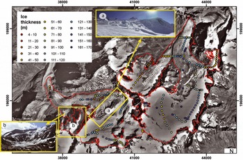
Fig. 2. Spatial distribution and results of ice thickness measurements for Mittelbergferner and Taschachferner in the Ötztal Alps. Data gaps on Taschachferner result from large crevasse zones and steep areas (small photographs).
Data interpolation
The point measurements were interpolated to calculate the total glacier volume. As shown in Figure 2, the measured point data are often sparse and unequally distributed over the glacier. Additional information is drawn from the natural boundary condition that the ice thickness is zero at the glacier margins. However, in regions with sparse data, automatic interpolation with algorithms (e.g. kriging, inverse distance weighting (IDW) or spline) produces ice thickness maps that deviate considerably from what can be expected from an educated guess. For example, crevassed areas can indicate discontinuities in the bedrock, and ice thickness in steep areas is usually smaller than in neighbouring flat areas. Furthermore, slopes of side-walls exposed during recent glacier retreat often suggest a constant slope, so the slope of the rocks surrounding the glaciers also provides information on the still ice-covered slope of the glacier bed. For hanging glaciers, the ice thickness at the front is apparent from the DEM of the glacier surface and the bedrock beneath. This information can be included, either by introducing artificial points for use in spatial interpolation algorithms or during manual construction of contours.
Another possibility is to interpolate measured data with the help of ice-dynamical models (e.g. Reference Binder, Bruckl, Roch, Behm, Schoner and HynekBinder and others, 2009; Reference Farinotti, Huss, Bauder and FunkFarinotti, 2009b). As the point data available for this study show inhomogeneous spatial distribution, and the method applied should be the same for every glacier, no such models have been used. Instead, 20 m contours of bedrock elevation were manually drawn (Fig. 3) for Taschachferner and Mittelbergferner according to point measurements and the following additional rules:
-
1. the ice thickness at glacier margins is zero
-
2. crevassed zones indicate ice thickness smaller than surrounding areas without crevasses
-
3. the slope of the surrounding bedrock indicates the slope of neighbouring ice-covered bedrock

Fig. 3. 20m contours of subglacial topography manually interpolated from the ice thickness measurements of Taschachferner and Mittelbergferner.
These contours were then interpolated with the ArcGIS tool ‘topo2raster’ on a 5 x 5 m2 grid (Fig. 4). The topo2raster tool is based on the ANUDEM algorithm developed by Reference HutchinsonHutchinson (1989). The ice thickness was then derived by subtracting the bedrock elevation DEM from the surface elevation DEM (using the ArcGIS tool ‘Minus’). The z-values of the nodes of the shapes of the glacier areas (without ice divides) were set to the value of surface elevation DEMs. Due to the difference between raster cells and node positions, the topo2raster interpolation often results in slightly negative ice thickness values. This was corrected by reclassification of these cells to an ice thickness of 2 m. The mean ice thickness, h, was calculated as the mean of the ice thickness, hN , at all N gridcells, and the maximum ice thickness as the maximum of all gridcells. The volume, V, of a specific glacier was calculated by multiplying the mean ice thickness, h, by the glacier area, A.

Fig. 4. Map of ice thickness of Taschachferner and Mittelbergferner calculated with the topo2raster tool.
Since all the volume data are intended for use in the glacier inventory, the area was taken from the glacier inventory even though the area changed between the GPR measurement and the date of the inventory. Thus the area assumed at the time of the measurements is too large, resulting in overestimation of the ice volume.
Uncertainty analysis
A rigorous and complete assesment of all errors and the uncertainty of the presented data based on sparse measurements would require a more thorough knowledge of a ‘true value’. What can be done to allow at least an estimate of the reliability of the presented volumes is an uncertainty analysis of (1) case studies and (2) the specific components leading to the results at point and glacier-wide level.
Calculation of the volume involves deriving the mean ice thickness for the glacier area by extrapolating the point measurements, and multiplying it by the glacier area. Thus the uncertainty involved in these two steps must be investigated.
Uncertainty of point ice thickness measurements
The ice thickness at one measurement location is calculated using Eqn (1) and involves mainly the following uncertainties:
-
1. the uncertainty of the signal velocity in the glacier, mainly due to the neglected firn and snow layers
-
2. the accuracy of the oscilloscope reading
-
3. the uncertainty of the antenna separation
-
4. unknown point of bedrock reflection
-
5. interpretation of multiple reflections.
Most of the measurements were carried out in winter, when the glacier was under seasonal snow cover. In the absence of a well-defined summer melt layer, snow probing does not allow the height of snow cover to be gauged, especially in the accumulation area. Thus the seasonal snow cover adds to the glacier thickness, in an order of 2 to ∼6m. Neglecting the signal velocities in firn (∼-200mp,s–1) and snow (∼290m μs–1) in Eqn (1) leads to an underestimation of ice thickness (Fig. 5) of up to 7 m, assuming a firn cover of 30 m and a snow cover of 5 m. In the case of winter snow cover, the overestimation of glacier volume by including the snow cover and the underestimation of the volume caused by the bulk velocity assumption can cancel each other out.
Fig. 5. Neglecting differences in signal velocities between ice, firn and snow leads to underestimation of the glacier thickness.
The accuracy of the oscilloscope reading depends on the ice thickness and is estimated at ∼30 ns with the Fluke 105 B oscillosope. The effects of uncertainties 3-5 on the accuracy can be high locally, especially on steep slopes, small and deep glacier tongues or in very rough bottom topography, so they are not considered further here. Overall, the uncertainty of point ice thickness measurements is assumed to be 5%, as the spatial interpolation method is regarded as the main uncertainty.
Uncertainty of data interpolation
The ice thickness was interpolated manually, after different interpolation methods had been tested in a case study for Schaufelferner. Schaufelferner has been surveyed several times with high data density, and the volume derived by manual contouring from the sparse GPR data was similar to the high-resolution volume. Automatic spatial interpolation algorithms (e.g. kriging, spline, natural neighbour or IDW) produce zero or negative ice thickness in areas where no measurements are available. Figure 6 shows examples for Mittelbergferner and Taschachferner. Geostatistical interpolation results in significantly underestimated volumes and mean ice thicknesses (Table 1). Even when the interpolation parameters can be optimized in the example, the ice thickness remains high close to GPR point measurements and decreases in unmeasured areas to zero. Averaging the GPR-measured ice thickness biases the volume towards higher values, since flat and central parts of the glacier show higher data density than crevassed and steep areas (Table 1). For both glaciers, the average of the mean ice thickness is 45 m and the results of all spatial interpolation algorithms are within 50% of the mean. This value can be considered the upper limit of uncertainty in mean ice thickness resulting from different data interpolation algorithms.
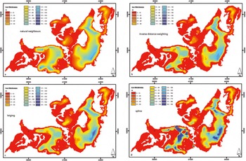
Fig. 6. Spatial interpolation algorithms as natural neighbours (a), IDW (b), kriging (c) and spline (d) underestimate ice thickness in unmeasured areas.
Table 1. Results of different methods to derive the mean (h mean) and maximum (h max) ice thickness, with standard deviation of the ice thickness
The same interpolation algorithm was used for all glaciers. The mean uncertainty of measured ice thickness was estimated to be 5% (Reference FischerFischer, 2009). Nevertheless, the main source of uncertainty in mean ice thickness is the unmeasured areas, since the mean ice thickness is calculated as the mean of all gridcells. Some gridcells are located close to measured values or known ice thickness (e.g. at the margins, where the ice thickness is zero), and should return lower uncertainties than those not surveyed. Assuming that one measured point represents a 250 x 250 m2 area with 5% uncertainty, an area-weighted mean uncertainty was calculated for the total glacier area assuming that the uncertainty in unmeasured areas is 50%.
Uncertainty of resulting volume
The uncertainty, aV, of the volume, V, is determined by the uncertainties, h , of the mean ice thickness, h, and the uncertainties, A, of the area, A
The area change between the date of the GPR measurement and the date of the glacier inventory was corrected assuming mean ice thickness for the lost area.
For glaciers not included in GI III so far, a mean decadal area change of 15% and a mean annual surface elevation change of -0.3 m a- 1 were assumed for the years between the first glacier inventory (GI I) and GI II, and - 0.9 m a -1 thereafter. Thus, the overall uncertainty of the glacier volume is
Reference Abermann, Lambrecht, Fischer and KuhnAbermann and others (2009) estimate σA/A as ±1. 5% for glaciers larger than 1 km2, and ± 5 . 0% for smaller glaciers. With the uncertainty of the mean ice thickness given above, the volume uncertainty is calculated in Table 2.
Table 2. List of surveyed glaciers with year of survey, number of point measurements (#), point measurements per square kilometre, year of glacier inventories and GPR measurements, and area (AA) and mean altitude (Ah) change between radar survey and DEM acquisition. For glaciers not included in GI III so far, mean values were calculated
Results and Discussion
For all 64 glaciers surveyed between 1995 and 2010 (Table 1) the measured data were interpolated to the total glacier area as described above. The number and spatial distribution of the measurements differ between glaciers as a result of accessibility. In crevassed areas, risky glacier travel and multiple reflections prohibited the survey. On and close to steep slopes, avalanches were a major concern, as well as fixing the antennas to the glacier surface. Figures 2 and 3 show the data recorded on Taschachferner and Mittelbergferner as typical examples of the data distribution. On Mittelbergferner, profiles along and across the glacier were measured. On Taschachferner, large crevasse zones and steep slopes prevented measurement along a central flow-line. Manual interpolation of the contours of bedrock topography allowed the estimated ice thicknesses at the vertical ice walls to be included and suggests that the crevasse zones are the result of a bedrock ridge (Fig. 2).
The surveyed glaciers cover areas of 0.001-18.4 km2. The mean thickness ranges from 10 to 92 m, and the maximum ice thickness from 26 to 311 m. For each surveyed glacier, area, mean and maximum ice thickness and the total volume are listed in Table 3. In total, the 64 glaciers cover an area of 2 2 3 . 3 ± 3 . 6 km 2 and contain a volume of 11.2 ± 1 . 1 km3. This would correspond to an average ice thickness of 5 0 ± 3 m if the ice were equally distributed.
Table 3. Areas, A (GI II), mean ice thickness, h (GI II), and volumes, V (GI II), calculated from the GPR data and corrected for area and volume change between the GPR measurements and the glacier inventory. The maximum ice thickness was not corrected with the local thickness change since that is not available for every glacier. The uncertainty of the maximum ice thickness, h max (GPR), is therefore higher, to correspond to the GI II volume data
Not only the total volume, but also the ice thickness distribution was calculated for all glaciers. The ice thickness maps of Mittelbergferner and Taschachferner are shown in Figure 4. Ice divides and glacier areas were assumed to be the same as in the glacier inventory to allow comparisons on a glacier-to-glacier basis. The ice divides in this study are therefore not considered to be flow divides but the glacier surface water divides mapped in the 1969 glacier inventory.
All spatial data were calculated in a very dense grid, although similar studies have used a spatial resolution of 25 m (Reference Farinotti, Huss, Bauder, Funk and TrufferFarinotti and others, 2009a). In this study, a nominal resolution of 5 x 5 m was chosen to avoid artefacts caused by different grid sizes used for the surface and bedrock DEM. The spatial resolution of the data differs from glacier to glacier, dependent on the number and distribution of ice thickness measurements. A grid size between 100 x 100 m2 and 250 x 250 m2 would thus have been more appropriate, but would then have resulted in mismatches with the glacier inventory data, especially for smaller glaciers. For most glaciers, the ice thickness data do not allow calculation of potential subsurface glacier lakes or routing of subglacial water flows. For specific analysis of features of the subglacial topography, higher data density and, to retrieve a higher spatial resolution of the subglacial topography, higher frequencies/smaller antenna footprints are recommended. Products of the compiled GPR data useful for glaciological application are, for example, altitudinal distributions of the ice volume, as shown for Mittelbergferner and Taschachferner in Figure 7.
Fig. 7. Mean and maximum ice thickness and glacier area in different altitude zones of Taschachferner and Mittelbergferner.
The number and distribution of survey points was governed by the topography of the glaciers, but since the thickest parts of the glaciers are usually located in flat areas with few crevasses, the maximum ice thickness will have been recorded for each glacier. Steep and crevassed areas usually show thinner ice cover. In some locations, the spatial coverage could be improved by helicopter surveys. In areas subject to multiple reflections (e.g. crevassed areas or areas close to bedrock), airborne radar cannot be expected to perform automatically better than ground-based measurements.
The comparison of the altitudinal distribution of ice thickness in Figure 7 demonstrates that the altitude zones with the highest mean and maximum ice thickness may differ from the zones with the largest areas. Therefore, including at least the vertical distribution of ice thickness should improve the reliability of future glacier area and volume change scenarios.
Conclusions and Outlook
Nearly two decades of GPR surveys have allowed the calculation of ice thickness data for a regional glacier sample. The data will be further extrapolated to compile a regional volume inventory. The resulting volume of 11.2 ± 1 . 1 km3 and the mean ice thickness of 50 m will then be extrapolated to the total Austrian glacier area, which is about twice that of the surveyed area. The surveys included a large portion of the largest glaciers, but also smaller glaciers, to be representative of Austria’s glaciers. The glaciers not measured to date are either small, difficult to access, steep or crevassed. Further investigations will focus on the best method for extrapolating these data. Algorithms as presented by Reference Farinotti, Huss, Bauder, Funk and TrufferFarinotti and others (2009a) and Huss and Farinotti (in press) are valuable approaches to modeling regional gridded ice thickness data. The data presented in this study can also be used as validation data for these algorithms. For example, the ice thickness data could help to investigate the effect of different glacier inventory dates, which is of special concern in current glacier retreat. The strength of the presented data lies in the fact that glacier areas, surface elevations and ice thickness data are derived consistently on the basis of the same dataset and recorded within a few years.
Acknowledgements
N. Span, M. Butschek, J. Lang, M. Massimo and S. Erhart carried out part of the GPR measurements. This work would not have been possible without the many helpers during several years of campaigns. K. Helfricht and M. Stocker helped with data processing. The field campaigns on Austrian glaciers were funded by the Commission of Geophysical Research, Austrian Academy of Sciences.


