


Introduction
Glide-snow avalanches release due to a loss of friction at the interface between the snowpack and the ground. Glide cracks (tensile fractures) sometimes form before an avalanche releases and can be a precursor to release (in der Gand and Zupančič, Reference in der Gand and Zupančič1966). Glide-snow avalanches pose a problem because of their destructive potential for infrastructure in alpine regions (Clarke and McClung, Reference Clarke and McClung1999; Mitterer and Schweizer, Reference Mitterer and Schweizer2012; Techel and others, Reference Techel, Pielmeier, Darms, Teich and Margreth2013), a lack of suitable mitigation measures (Clarke and McClung, Reference Clarke and McClung1999; Sharaf and others, Reference Sharaf, Glude and Janes2008; Simenhois and Birkeland, Reference Simenhois and Birkeland2010) and unreliable forecasting capabilities (Jones, Reference Jones2004; Simenhois and Birkeland, Reference Simenhois and Birkeland2010).
It is generally assumed that the loss of friction between the snowpack and the ground is due to the presence of liquid water at this interface. The source of liquid water depends on the season (Clarke and McClung, Reference Clarke and McClung1999). When the snowpack is dry (so-called ‘cold temperature’ events typically occurring in early winter), the heat stored by the soil is thought to melt the adjacent snowpack (McClung, Reference McClung1987; Newesely and others, Reference Newesely, Tasser, Spadinger and Cernusca2000; Höller, Reference Höller2001) or a difference in hydraulic pressure between snow and soil could cause a wetting of the lowermost snow layer (Mitterer and Schweizer, Reference Mitterer and Schweizer2012). When the snowpack temperature is at $0^\circ$ C (so-called ‘warm temperature’ events typically occurring in spring), meltwater or rain percolates through the snowpack and accumulates at the snow-ground interface (Lackinger, Reference Lackinger1987; Clarke and McClung, Reference Clarke and McClung1999). Other mechanisms such as lateral flow from underground springs are possible sources of interfacial water throughout the season (McClung, Reference McClung1987). Although these hypotheses are widely accepted, there is little understanding of the dominating underlying processes and their timescales. One reason for this limited understanding is that field observations are based on few or single events (Ancey and Bain, Reference Ancey and Bain2015).
The limited number of observations often lead to ambiguous and sometimes contradictory statements between publications. For example, there have been reports of higher glide activity during the evening and at night (Lackinger, Reference Lackinger1987), higher glide rates during the day (McClung and others, Reference McClung, Walker and Golley1994; Feick and others, Reference Feick, Mitterer, Dreier, Harvey and Schweizer2012), and no significant difference in glide rate activity between night and day (Clarke and McClung, Reference Clarke and McClung1999). Another example is the use of glide rates as predictors for avalanche release (Endo, Reference Endo1984; Lackinger, Reference Lackinger1987; Nohguchi, Reference Nohguchi1989; Kawashima and others, Reference Kawashima, Iyobe and Matsumoto2016). Reported indicators for avalanche release include the exceedance of a critical glide rate (in der Gand and Zupančič, Reference in der Gand and Zupančič1966), glide rate acceleration before release (Stimberis and Rubin, Reference Stimberis and Rubin2011; van Herwijnen and others, Reference van Herwijnen, Berthod, Simenhois and Mitterer2013) or no clear relationship between glide rate and release (McClung and others, Reference McClung, Walker and Golley1994; Clarke and McClung, Reference Clarke and McClung1999).
To reduce the ambiguity within observations using statistics, time-lapse photography is a well suited method to increase the number of recorded glide events. Compared to alternative methods like glide-shoes (in der Gand and Zupančič, Reference in der Gand and Zupančič1966) or terrestrial radar interferometry (Caduff and others, Reference Caduff, Wiesmann, Bühler, Bieler and Limpach2016), time-lapse photography is simple, low cost and can be used to continuously monitor large areas as long as there is sufficient visibility. For some case studies, it has been shown that glide dynamics can be extracted from time-lapse photographs (van Herwijnen and Simenhois, Reference van Herwijnen and Simenhois2012; van Herwijnen and others, Reference van Herwijnen, Berthod, Simenhois and Mitterer2013). However, this method has not yet been used to comprehensively investigate glide-snow avalanches and glide dynamics at various timescales.
Our aim is to use time-lapse photography to characterize glide-snow avalanches and glide dynamics across different timescales (annual, intra-seasonal, diurnal and sub-hourly). To this end, we present a semi-automated, pixel-based algorithm to detect glide events and extract glide rates from time-lapse photographs. The algorithm is based on Otsu's method (Otsu, Reference Otsu1979) combined with a shadow correction, a temporal correction and pixel clustering. The spatial resolution after georeferencing is ~0.5 m and the temporal resolution is 2–15 min. The algorithm was applied to a time-lapse photography dataset from Dorfberg (Davos, Switzerland) spanning 14 seasons (2009–22). This resulted in 947 glide events (including avalanches and glide cracks) and glide rates for 123 events.
Methods
Study site and dataset
The study site is Dorfberg, a mostly southeast-facing mountainside above Davos (Switzerland) where glide-snow avalanches often release at elevations ranging from 1650 to 2100 m a.s.l. (Fig. 1). The mean slope angle of the monitored area is $(31 \pm 9)^\circ$ (mean ± std dev.). The slopes where glide-snow avalanches were observed are steeper ($(39 \pm 6 )^\circ$
 ). Most slopes are open meadows that are interspersed with shrubs, rocky areas and open forests (Feistl and others, Reference Feistl, Bebi, Dreier, Hanewinkel and Bartelt2014). The snow climate in Davos can be defined as transitional to continental with an annual mean precipitation of 1452 mm (75% in solid form) and a mean temperature of $-1.1^\circ$
 C recorded between 2009 to 2022 at Weissfluhjoch (2536 m a.s.l., located 2 km northwest of Dorfberg). Time-lapse photographs of Dorfberg were taken from 2009 to 2022 (winter season 2008/09 is denoted as 2009), with time intervals ranging from 2 to 15 min. The camera (pixel resolution in Table 1) was installed inside a building at the Institute for Snow and Avalanche Research SLF and is located 1 km line of sight from Dorfberg (Fig. 2).

Figure 1. Southeast facing slope of Salezerhorn (2536 m a.s.l.) called Dorfberg (Davos, Switzerland).

Figure 2. Heatmap of number of glide-snow avalanches on Dorfberg (2009–22) and the position of the virtual stations for SNOWPACK simulations (see ‘Methods’). The location of the camera (Cam) is indicated in red. Coordinates: CH1903+, Map: swisstopo.
Table 1. Pixel resolution of installed cameras

To extract the location and dynamics of glide-snow avalanche release, a pixel-based detection algorithm was implemented to detect snow-free pixels in every image.
Pixel-based algorithm
The algorithm automatically separates pixels that are continuously snow-covered and pixels that change their state from snow-covered to snow-free (e.g. opening glide crack, released glide-snow avalanche, snow melting on trees or rocks). In order to detect snow-free pixels, a reference image where all pixels of interest are snow-covered, an event image where the pixels are not covered by snow anymore, and a manually selected region of interest (ROI) around the event are required. The algorithm consists of four steps (Fig. 3): (1) Otsu's threshold to distinguish between snow-covered and snow-free pixels, (2) a shadow correction, (3) a temporal correction to reduce the fluctuation of the number of detected pixels between subsequent images and (4) clustering of neighbouring pixels to select large snow-free pixel clusters. These clusters can be related to glide cracks and glide-snow avalanches.

Figure 3. Overview of the input data, algorithm processing steps, output data and the postprocessing.
Otsu's threshold
The pixels are separated between snow-covered and snow-free pixels based on their value in the HSV (hue, saturation and value) colourspace. The value (v ∈ [0, 255]) corresponds to the colour brightness. We assume that every ROI can be represented by a bimodal value distribution consisting of snow-covered and snow-free pixels (Fig. 4a). The optimal threshold to separate a bimodal distribution can be calculated using Otsu's threshold which maximizes the inter-class variance (Otsu, Reference Otsu1979). All pixels with values smaller than the threshold were classified as snow-free while all pixels with values greater than the threshold were classified as snow-covered. The bimodal distribution and the optimal threshold shift between images due to changes in illumination or weather conditions. For this reason Otsu's threshold is applied on every image. After the application of Otsu's threshold to the reference image and the event image, both images are compared pixel-wise to select the pixels that changed their classification from snow-covered to snow-free. These are the pixels of interest.

Figure 4. Images (top) of an opening glide crack and their corresponding value (v, corresponds with brightness) distributions (bottom) with different shadow conditions. (a) The glide crack image is not influenced by shadows. Its value distribution can be interpreted as bimodal and can be separated with Otsu's threshold (v snow-free ∈ [0, 136] and v snow-covered ∈ [137, 255]). (b) The glide crack image is influenced by shadows and its value distribution is not bimodal. The separating threshold is set to a value of 115 as part of the shadow correction (dashed line). This results in the separation of v snow-free ∈ [0, 115], v shadow ∈ [116, 159], v snow-covered ∈ [160, 255].
Shadow correction
A limitation for Otsu's method is the presence of local shadows within the ROI. The brightness of a shaded snow area is lower than the brightness of the surrounding snow. This changes the pixel brightness distribution from bimodal to trimodal (Fig. 4b), which no longer fulfils the bimodal requirement for Otsu's method. This causes a misclassification of some shadows as snow-free and a severe overestimation of the number of snow-free pixels (Fig. 5a). As shadows are common throughout the day in complex topography, a correction is needed.

Figure 5. Image processing workflow illustrated by an image with detected snow-free pixels (yellow, top row) throughout the steps of the algorithm: (a) Otsu's method, (b) shadow correction and (c) temporal correction. The classification into snow-covered (0) and snow-free (1) over time is shown for three pixels (middle row). The green pixel is in a continuously snow-covered region which is influenced by shadows. The red and purple pixels turn snow-free at different time steps and are also influenced by shadows. The bottom row shows the number of snow-free pixels for every time step. The time of the image in the top row (18 January 2012, 15:00) is indicated by the grey line. Time steps when the shadow correction was applied are indicated by orange dots.
Shadows can be detected through the saturation of a pixel. If more than 2% of pixels in the ROI had a saturation between 37 and 54, and the image was taken between 11:30 and 16:00, the threshold value to distinguish snow-covered from snow-free pixels was set to 115 (Fig. 4b). The saturation range and the shadow threshold were determined empirically based on observations in images with extreme shadow events. If a majority of pixels ($\gtrsim \! 70$ %) in a ROI are detected as possible shadows, the value distribution is close to bimodal and Otsu's method can be applied without corrections.
Temporal correction
When evaluating snow-free pixels over several images, the number of detected pixels in subsequent images fluctuates (Fig. 5b). There are several reasons for this. First, the shadow correction is not perfect as it assumes two manually set parameters, namely the saturation of shadow pixels and the constant threshold. Second, small changes in the focus of the camera can slightly shift the position of pixels which causes the edges of snow-free areas to sometimes be part of a pixel and sometimes not. The fluctuations can be reduced with a temporal correction.
The temporal correction requires subsequent time-lapse images and assumes that a snow-free area can only increase in size. For an event image, the classification of every single pixel is evaluated for a number of subsequent event images (N). Only if a pixel is continuously classified as snow-free throughout all N subsequent images will it be classified as snow-free in the event image. The temporal correction works best when the time range covered by N images balances out very short-term changes in illumination and shadows. For our evaluation, a time range of 1–2 h showed stable results (e.g. N = 12 − 24 given a 5 min interval between images). The temporal correction reduces the noise of the detected pixels and displays the underlying glide-event dynamics (Fig. 5c).
Clustering
By design, the algorithm detects all pixels that change their classification from snow-covered in the reference image to snow-free in the event image. Glide cracks or avalanches are large continuous snow-free areas. To further limit the number of misclassified pixels, pixel clusters with <5% of the number of pixels of the largest cluster were removed automatically. Clusters were determined as connected pixels taking into account only first-order neighbours. In case the previous corrections were not sufficient, a final option within the algorithm allows for manual masking of misclassified regions.
The combination of Otsu's method, the shadow correction, the temporal correction and the clustering resulted in a robust algorithm that automatically detected snow-free pixels. The snow-free pixels can be linked to glide events like opening glide cracks or glide-snow avalanches (Fig. 5c).
Postprocessing
Georeferencing and glide dynamics
After the snow-free pixels of a glide event were identified, the image was georeferenced to convert the pixel locations to real-world coordinates. This was achieved using the monoplotting tool (Bozzini and others, Reference Bozzini, Conedera and Krebs2012) on a DEM (resolution 0.5 m × 0.5 m). To validate the image processing workflow and georeferencing, detected release areas were compared to the same areas recorded in drone orthophotos. The orthophotos were available for four glide-snow avalanches in season 2022 and they were taken 2–3 days after the avalanche events with a resolution of 3 cm × 3 cm (Table 2). The area extracted using the algorithm and georeferencing was 3–28% smaller than the area extracted from the orthophotos, and differences decreased with the size of the area.
Table 2. Comparison of area extracted from images with the pixel-based algorithm and from drone orthophotos

The difference is calculated by (A image − A ortho)/A ortho.
Glide distances were extracted separately along the horizontal and vertical direction of the georeferenced time-lapse photographs. In the majority of cases, these directions align with the width and length (downslope) of the glide cracks and glide-snow avalanches. The corresponding glide rates were calculated by dividing the downslope (length) glide distance with the time interval between images. We evaluated the glide distance at different positions along a glide crack. This showed that the glide distance evolution was highly dependent on the location along the crack and the glide crack geometry (Fig. 6). Therefore, we determined the glide distance and glide rates by taking the mean across the entire glide crack.

Figure 6. Glide distance recorded at different positions in the glide crack. The positions are given as a fraction of the glide crack width ranging from 0.1 to 0.9 (colours purple to yellow). The mean glide distance over the entire glide crack width is indicated in black. The glide crack is the same as in Figure 5.
To characterize the glide crack dynamics before avalanche release, we investigated the change in glide crack aspect ratio (Δwidth/Δlength) and the downslope (length) crack opening dynamics. The change in aspect ratio was calculated as the slope of a linear fit to the width-length plot of an opening glide crack (Fig. 7). The change in aspect ratio was considered to be constant if the standard error of the slope was smaller than 0.2. The downslope opening dynamics were quantified with a best-fit approach. Opening glide cracks with a sufficient crack opening duration (more measurement points than fit parameters) were fit with an exponential, a linear, and an asymptotic exponential function. These functions were chosen based on the repeated patterns that emerged from visually inspecting the dataset. For cracks that released as an avalanche, only the glide distance development before avalanche release was taken into account (Fig. 8a). The best fit type for every glide distance evolution was determined using the lowest residual standard error (examples in Fig. 8, first row).
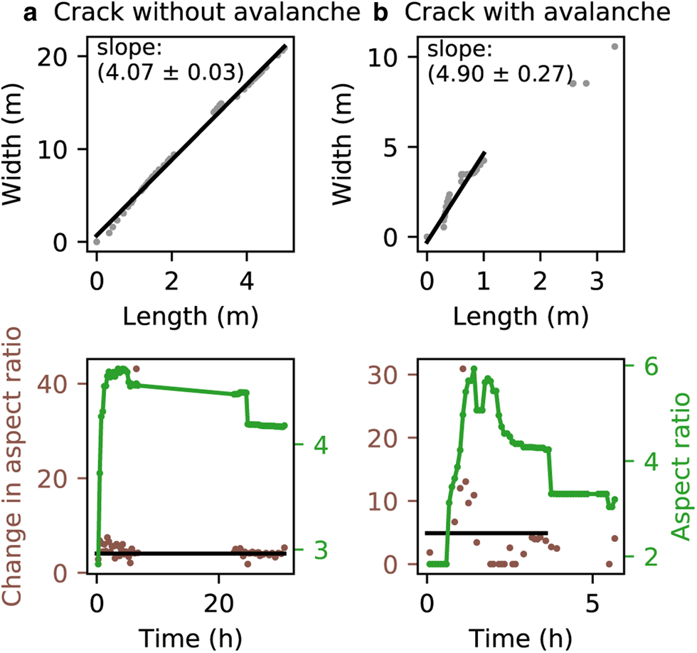
Figure 7. Change in glide crack aspect ratio (Δwidth/Δlength) was determined as the slope of the width–length plot. (a) An example for a crack without avalanche release where the change in aspect ratio is constant (slope standard error <0.2). The bottom row shows the change in aspect ratio (brown scatter plot) and aspect ratio (green line plot) over time. The change in aspect ratio, as determined from the fit, is also shown in the bottom row (black line). (b) An example of a crack before avalanche release where the change in aspect ratio is not constant (slope standard error >0.2).

Figure 8. Examples of best fits of the downslope (length) glide distance: (a) crack opening with overall exponential behaviour before release; (b) linear behaviour and (c) asymptotic behaviour for two glide cracks without avalanche release.
Surface-generated interfacial water (surface events) versus interface-generated interfacial water (interface events)
Glide events are typically classified as ‘cold’- or ‘warm’-temperature events (e.g. Clarke and McClung, Reference Clarke and McClung1999). The original definition (Clarke and McClung, Reference Clarke and McClung1999) combined air temperature and the source of interfacial water. Later publications manually assigned events to one category based on air temperatures (Ceaglio and others, Reference Ceaglio2017) and the snow temperature in manually observed snow profiles (Dreier and others, Reference Dreier, Harvey, van Herwijnen and Mitterer2016). This manual classification is prone to subjective interpretation and is not reproducible. We therefore developed an objective classification method based on meteorological measurements and simulated snow stratigraphy.
We simulated snow stratigraphy using the numerical snow cover model SNOWPACK (Bartelt and Lehning, Reference Bartelt and Lehning2002) for all 14 seasons at eleven virtual stations across Dorfberg, which were positioned in frequent glide-snow avalanche release areas (Fig. 2). SNOWPACK (V3.60, research mode) simulations were initiated without soil and based on the meteorological measurements from two IMIS stations in the vicinity: Weissfluhjoch (WFJ2, 2536 m a.s.l., ~2 km distance) and Madrisa (KLO2, 2147 m a.s.l., ~10 km distance). The simulations were validated during one season (2022) with weekly manually observed snow profiles. More details on the SNOWPACK simulation setup and validation are given in Appendix A. SNOWPACK simulations showed that using air temperature or whether the snowpack is isothermal (temperature across the entire snowpack at $0^\circ$ C) was not sufficient to describe the source of interfacial water. There were occasionally time periods when interfacial water from meltwater percolation was present, yet the snowpack above was partly cold (Fig. 9, e.g. 6 and 8 February 2017). Based on previously applied classifications, events during such a time period would have been classified as ‘cold’, as there was no surface melt. However, the interfacial water resulted from prior surface meltwater which had percolated to the basal layers.

Figure 9. SNOWPACK simulation of (a) daily mean liquid water content (LWC) that shows the percolation of surface meltwater down to the basal snow layer (starts on 2 February 2017). Glide events during this time period would be classified as surface events due to the source of the basal water. Note that the classification is solely based on the source of the interfacial water and not on (b) the snow temperature. As a result, the snowpack can be partly cold (e.g. 6 and 8 February 2017) for surface events. Snowpack temperatures of 0$^\circ$ C are indicated in red.
We thus propose to classify glide-snow events according to the source of the water, namely ‘surface-generated interfacial water’, in short surface events, and ‘interface-generated interfacial water’, in short interface events. Surface events can be attributed to liquid water originating from surface melt that percolated through the snowpack. Interface events are not associated with meltwater from the snow surface. The water at the base of the snowpack in interface events could have therefore originated from interfacial melt from geothermal heat flux (McClung, Reference McClung1987) or suction (Mitterer and Schweizer, Reference Mitterer and Schweizer2012). These latter processes are not accounted for in our SNOWPACK simulations.
We applied this new classification to the SNOWPACK simulations using a threshold based on the liquid water content of the snowpack. In our simulations, an increase in liquid water content was always due to surface melt as the SNOWPACK simulations were initiated without soil and with the bucket-approach for water percolation (Bartelt and Lehning, Reference Bartelt and Lehning2002). Every glide-snow event was assigned to the most representative virtual station based on distance to the virtual station and similarity in elevation, aspect and slope. When it was not possible to assign a station (e.g. low visibility, difficulty georeferencing the event), the mean of all stations was used to classify the event. Events were classified as an interface event when all of the following criteria were fulfilled for the daily mean values in the simulated snowpack:
(1) The simulated snow layer closest to the ground had a liquid water content of 0%.
(2) Less than 5% of simulated snow layers in the upper half of the snowpack had a liquid water content above 0%.
(3) Less than 5% of simulated snow layers in the lower half of the snowpack had a liquid water content above 0%.
All other events were classified as surface events, as we could not exclude that water at the base of the snowpack originated from surface melt.
Results
The image processing workflow consisting of the pixel-detection algorithm, the postprocessing steps and the surface/interface event classification was applied to the Dorfberg time-lapse photography dataset. This resulted in a total of 947 glide-snow events (650 surface events/297 interface events). These events consisted of glide-snow avalanches that released immediately (<15 min of prior crack formation), glide cracks that developed for more than 15 min and released as an avalanche, and glide cracks without avalanche release. Glide cracks were used for glide distance calculations if they included more measurement points than fit parameters and if they released on slopes directly facing the time-lapse camera. The georeferencing was unreliable on slopes not facing the camera. Immediate-release glide-snow avalanches accounted for 516 (374/142) events. Glide cracks that released as an avalanche accounted for 267 (178/89) events, of which 61 (33/28) events were suitable for glide rate calculation. Glide cracks without avalanche release accounted for 103 (57/46) events, of which 51 (34/17) were suitable for glide rate calculation.
Annual glide-snow avalanche activity
The glide-snow avalanche activity varied substantially between the 14 seasons in terms of the number of events as well as the surface/interface event ratio (Fig. 10). The glide events were separated into three categories: glide-snow avalanches that released immediately (516), glide cracks that released as an avalanche (267) and glide cracks that did not release as an avalanche (103). On average, 54% of glide-snow avalanches released immediately and surface events were more likely to release immediately (59%) than interface events (48%, Fig. 10). If a glide crack opened, it was two times more likely to release as an avalanche than not to release (Fig. 10). Although glide-snow avalanche activity varied substantially between years, there were a few noteworthy details. First, in 2015, many immediate release surface events occurred. The majority (n = 55) of these events released on a single with very high glide-snow avalanche activity in November 2014 (Figs 10, 11). Second, in 2012, the highest number of glide cracks without avalanche formation occurred (n = 14, Fig. 10). This season was also characterized by continuous glide-snow avalanche activity throughout the season as well as large snow depths (Fig. 11). Third, overall glide-snow avalanche activity was the lowest in seasons 2014 and 2022 (Fig. 10). Both seasons showed little glide-snow avalanche activity after the first snowfall, a low snow depth, and an early melt-out date (Fig. 11).

Figure 10. Number of surface and interface events separated by type of release (immediate release, crack followed by avalanche and crack) varied substantially between years. The mean percentage of release type for all seasons is given in the legend for surface and interface events (n = 947).

Figure 11. Daily glide-snow avalanche activity for all seasons and the snow depth of all virtual stations (ordered with descending snow depth: VIR6, VIR10, VIR9, VIR3, VIR8, VIR4, VIR7, VIR5, VIR1, VIR2). The snow depth is coloured in orange (time period when events were classified as surface events) and blue (interface events). The points indicating the daily number of observed glide-snow avalanches are also coloured, indicating how the majority of glide-snow avalanches were classified based on their closest virtual station.
Glide-snow avalanche activity within a season
In most winter seasons where images were available in early winter, a first cluster of glide-snow avalanches occurred in October or November. The avalanches often released within a few days of a snowfall on snow-free ground (e.g. 2014, 2018, 2019, 2021, 2022, Fig. 11). Such a period was then followed by multi-day clusters of events throughout the winter season. Only season 2022 experienced a mid-winter (January and February) period without glide events. The classification of the glide events into surface and interface events showed that the potential source of interfacial water can change several times throughout the season depending on the location and the meteorological conditions. As expected, the events in spring, after the snowpack had reached its isothermal state, were classified as surface events. In addition, the snowfall on snow-free ground was often classified as a surface event (e.g. season 2014, 2015, 2019, 2021) due to mild air temperatures in combination with shallow snow depths. Interface events commonly occurred between November and early February. Overall, glide-snow avalanche activity was highly variable depending on the winter season.
Diurnal glide-snow avalanche activity
Glide-snow avalanche activity occurred during all daylight hours and also during the night (Fig. 12). Fewer glide-snow avalanches released during the night (defined as 19:00–07:00; surface events: 18%, interface events: 14%) than during the day. Glide-snow avalanches were more likely to release during the afternoon hours (13:00–18:00, surface: 50%, interface: 52%) than the morning hours (07:00–12:00, surface events: 32%, interface events: 34%).

Figure 12. Time of glide-snow avalanche release separated into surface (n = 650) and interface events (n = 297).
Crack opening duration
Around half (54%) of the recorded glide-snow avalanches released immediately, without prior crack formation (Fig. 10). Focusing on avalanche events with prior glide-crack formation (n = 267) showed that, within the first 24 h after initial crack formation, 67% of the cracks had released as an avalanche (Fig. 13). The separation between interface and surface events showed that surface events had a higher probability of avalanche release within 24 h of initial crack opening (surface events: 81% within 24 h, interface events: 63% within 24 h).

Figure 13. Cumulative relative frequency of avalanche release versus the time between initial crack opening and avalanche release. The relative avalanche frequency was fit (solid line) with an exponential function (f(x) = A + B ⋅ exp( − αx)). The fit parameters are given in Table 3.
Table 3. Fit parameters of cumulative relative frequency (Fig. 13)

Glide dynamics: downslope
Glide rates were extracted for 112 glide cracks (61 followed by an avalanche, 51 without avalanche) and separated into surface and interface events (Fig. 14). For glide cracks that released as an avalanche, only glide rates prior to avalanche release were taken into account. Glide rates of 0 mm h−1 accounted for three quarters of all observed glide rates. The large number of 0 mm h−1 glide rates suggests an overall stick–slip behaviour in the glide crack opening dynamics. Cracks suddenly opened and then found a new equilibrium position where no further gliding was recorded. This stick–slip behaviour is also visualized in the extracted glide distances (e.g. Figs 6, 8). Excluding the 0 mm h−1 glide rates, the observed glide rates were below 600 mm h−1 in most cases (90%). In a few cases, glide rates reached up to and also exceeded 800 mm h−1 although the glide rates did not include glide-snow avalanche releases. The glide rate distributions of surface/interface events differed significantly (p < 0.01 Mann–Whitney U test, without 0 mm h−1 glide rates). Overall, glide rates for surface events showed higher mean and median values than interface events (Fig. 14). The overall glide crack opening dynamics were quantified with the best-fit of an exponential, linear and asymptotic function. This approach showed that cracks exhibiting exponential behaviour had a 80% probability to eventually release as an avalanche (Fig. 15). However, only 43% of glide cracks that later released as an avalanche showed exponential behaviour. The linear and asymptotic fits did not provide a clear indication for avalanche release.

Figure 14. Frequency of hourly glide rates (n = 58 187) from opening glide cracks (n = 112). Glide rates were computed from opening glide cracks without avalanche release and from opening glide cracks with avalanche release before avalanche release occurred. The interface/surface event distributions differ significantly (p < 0.01, Mann–Whitney U test). The mean, median and Mann–Whitney U test were calculated without glide rates of 0 mm h−1.

Figure 15. Number of cracks that released as an avalanche or did not release as an avalanche depending on the best fit to their glide distance dynamics. Only fits with a residual standard error smaller than 0.3 were taken into account (n = 91).
Glide dynamics: change in aspect ratio
The glide crack development was characterized by a linear relationship between the glide crack width and its length (Fig. 7). The change in aspect ratio (Δwidth/Δlength) was constant (standard error of slope <0.2) for 88% of glide cracks without avalanche release and for 57% of glide cracks with eventual avalanche release (Fig. 16). For interface events, all opening glide cracks without avalanche release had a standard error below 0.2 (Fig. 16). Regarding the magnitude of the change in aspect ratio, interface glide cracks without avalanche release showed significantly higher changes in aspect ratios than cracks with avalanche release (p = 0.001, Mann–Whitney U test, Fig. 17a). This difference was less prominent for surface events (p = 0.09). There was also no substantial difference comparing the surface and interface distributions. A few cracks that were classified as surface events showed very large changes in aspect ratio. The geometry of released glide-snow avalanches (without their runout) was mostly characterized by a similar width and length which resulted in small aspect ratios and a narrow aspect ratio distribution (Fig. 17b).

Figure 16. Relative frequency of the standard error of the change in aspect ratio (Δwidth/Δlength) for developing glide cracks with and without avalanche release (see Fig. 7 for the standard error calculation). The threshold for constant incremental change in aspect ratio (standard error <0.2) is indicated in black (sample size: crack (surface: 34/interface: 17), crack with avalanche (33/28)).

Figure 17. Violin plot showing (a) the distribution of the change in aspect ratio (Δwidth/Δlength) separated into cracks (without avalanche release) and cracks before avalanche release by surface/interface classification. (b) For released avalanches the final aspect ratio is given. The quartiles (Q1, Q3) are indicated with a dotted line and Q2 (median) with a dashed line (sample size: crack (surface: 34/interface: 17), crack with avalanche (33/28), avalanche (316/105)).
Discussion
Pixel-detection algorithm and surface/interface classification
The pixel-based algorithm automates the glide crack/avalanche detection based on the manual input of the ROI and the reference picture. We manually selected the ROI for every event around the avalanche or crack because the algorithm (by design) also detects pixels that are snow-free due to melt. As the snowpack on Dorfberg is typically shallow (mostly below 1.5 m, see snow heights for all virtual stations in Fig. 11), the formation of larger snow-free areas on/around rocks throughout the mountainside and due to melt was common. In addition, using an ROI reduced the computation time during the temporal correction, especially for long-opening cracks and high-resolution images. The manual ROI selection is not necessary if the algorithm is applied to one specific slope or areas where there is no melt out (e.g. no large rocks, large snow depths). The detected glide-snow avalanche release areas were systematically smaller than the same areas detected on drone orthophotos (Table 2). This may be because of occlusions as the camera looked at Dorfberg from below and was mounted at 1 km of line of sight distance from Dorfberg. The increasing difference with decreasing area may be due to the increased importance of small errors (georeferencing, changes in focus of the camera, occlusion).
Through the application of the algorithm to time-lapse images of Dorfberg, we created a comprehensive dataset of glide-snow avalanches and glide rates. However, our dataset is based on only one site (Dorfberg) and is limited in the range (mean ± std dev.) of aspects (($125\pm 30) ^\circ$ ), slope angles (($31\pm 9) ^\circ$
 ) and elevations ((1983 ± 166) m a.s.l.) which may bias our results.
Due to the large number of glide events, they were automatically classified depending on their suspected source of interfacial water. The classification was based on our current understanding of the source of interfacial water by applying a threshold to the snow-liquid water content simulated with SNOWPACK. For a better, process-based separation of glide-snow events, a better understanding of the source of interfacial water, its quantity and its spatial distribution is needed.
While we used daily values of the SNOWPACK simulations at various locations across Dorfberg, we could only validate the simulations on a weekly basis at one location during season 2022 with manually observed snow profiles. These profiles were qualitatively in good agreement with simulated snow stratigraphy (Fig. 18 in Appendix A).

Figure 18. Comparison of traditional snow profiles recorded in the field and simulated SNOWPACK profiles. (Abbreviations for grain types: PP, precipitation particle; DF, decomposing and fragmented precipitation particles; RG, rounded grains; FC, faceted crystals; DH, depth hoar; SH, surface hoar; MF, melt forms; IF, ice formations.)
Avalanche activity
Glide-snow avalanche activity varied substantially between the years, which is in line with results presented by Mitterer and Schweizer (Reference Mitterer and Schweizer2012). This may be due to highly variable meteorological conditions (Höller, Reference Höller2001) which may influence the availability of interfacial water. For example, 55 glide-snow avalanches released during one night in early November 2014 (Fig. 11). These events occurred after the first snowfall of the season which occurred in combination with mild air temperatures. This could have resulted in interfacial water originating from melt of the snowpack on the ground as well as from surface melt. The events were classified as surface events which indicates there was indeed an increased liquid water content in the snow due to surface melt. The combination of two sources of liquid water could have contributed to a loss of friction across Dorfberg. In addition, it was the first snowfall of the season which indicates that the snowpack had a lower density than in spring. Low-density snow is generally fragile, suggesting a weak stauchwall zone (Bartelt and others, Reference Bartelt, Feistl, Bühler and Buser2012), which would also favour glide-snow avalanche release. There are three additional seasons we would like to point out. First, season 2011/12, which was characterized by high glide-snow avalanche activity in Switzerland (Techel and others, Reference Techel, Pielmeier, Darms, Teich and Margreth2013). On Dorfberg, we recorded numerous interface events (overall second largest number) and the largest number of opening glide cracks without avalanche release (interface events, Fig. 10). The interface events were distributed throughout most of the season (Fig. 11). Second, season 2018/19, which was also characterized by high glide-snow avalanche activity (Zweifel and others, Reference Zweifel2019). On Dorfberg, we recorded an average number of glide-snow events, but the glide-snow avalanche activity was again continuous throughout the entire winter (Fig. 11). Third, season 2022 was an example for a season with low avalanche activity (Fig. 10). This season was characterized by below average snow depth and repeated melt out at lower elevations. Overall, in our data, yearly avalanche activity showed only slight positive, though not significant, correlation with maximum snow depth (Spearman, r s = 0.32, p = 0.27). This suggests that more parameters have to be taken into account to explain the variation in glide-snow avalanche activity.
Over the course of the day, glide-snow avalanches showed increased avalanche activity in the afternoon, which is in line with the overall observations of Feick and others (Reference Feick, Mitterer, Dreier, Harvey and Schweizer2012). In other publications, higher glide activity during the evening and night (Lackinger, Reference Lackinger1987) or little distinction in accumulated glide between day and night (McClung and others, Reference McClung, Walker and Golley1994; Clarke and McClung, Reference Clarke and McClung1999) were observed. The release timing may be influenced by the underlying process and source of interfacial water. For surface events, the meltwater produced at the snow surface may need time to form and percolate to the snow–ground interface, which makes an avalanche release in the afternoon hours more likely. In addition, the snowpack is exposed to large diurnal changes in air temperature and radiation, which can lead to diurnal changes in the snowpack properties associated with melt and refreezing. We would expect this effect to be less pronounced for interface events where the source of interfacial water (within our definition) is independent from diurnal fluctuations in radiation or air temperature, for example. However, we can also observe more interface avalanche releases towards the afternoon hours. This may indicate that effects like lateral flow of liquid water that forms through melt (e.g. near protruding rocks) may also be important.
Glide dynamics
It is well-known that glide cracks can form before the release of a glide-snow avalanche (e.g. van Herwijnen and others, Reference van Herwijnen, Berthod, Simenhois and Mitterer2013). However, in our dataset, less than half of the glide-snow avalanches included a visible glide crack before release. This result could be biased by the limitations of time-lapse photography including the image recording interval, the angle and distance to the camera, the crack location and the snow height. If the snow height is large and the terrain very shallow, the camera cannot record an opening glide crack because it is occluded. Consequently, the recorded number of glide-snow avalanches with prior crack formation should be seen as a lower limit.
We also observed that avalanche release became less likely with increasing crack opening duration (Fig. 13). This is in line with previous studies that reported opening duration from minutes to weeks (Lackinger, Reference Lackinger1987) to months (McClung and Schaerer, Reference McClung and Schaerer2006).
As accelerating glide rates have been considered as possible precursors for avalanche release (in der Gand and Zupančič, Reference in der Gand and Zupančič1966), we investigated the temporal evolution of glide rates in more detail. We were able to extract glide rates by georeferencing the time-lapse photographs. The minimum glide rates that can be recorded from time-lapse images depended on the spatial and temporal image resolution, the resolution of the DEM used for georeferencing, and the error introduced by georeferencing (Table 2). After georeferencing, one pixel, on average, had a length and width of 0.5 m each. This is an average across all camera resolutions (Table 1) and locations on Dorfberg. Depending on the topography, the length and width of a pixel can vary substantially and a square pixel in the image generally corresponds to a polygon area in the real world. Assuming an average resolution of 0.5 m in downslope direction, this results in a minimum detectable glide rate of 100 mm min−1 assuming a 5 min time interval between images.
Extracted glide rates distributed across opening glide cracks showed highly non-uniform behaviour depending on their location and the glide crack geometry (Fig. 6). This may indicate that traditional glide shoe measurements (in der Gand and Zupančič, Reference in der Gand and Zupančič1966) are highly location dependent and difficult to interpret. We extracted glide rates by taking the mean glide distance and mean glide rate across the entire glide crack width.
Glide rates reported in literature range from a few centimetres per day (Clarke and McClung, Reference Clarke and McClung1999) to 430–670 mm h−1 (Margreth, Reference Margreth2007; Stimberis and Rubin, Reference Stimberis and Rubin2011; Caduff and others, Reference Caduff, Wiesmann, Bühler, Bieler and Limpach2016). Of the extracted glide rates on Dorfberg, 90% were below 600 mm h−1, but more extreme values of up to and exceeding 800 mm h−1 were also observed (Fig. 14). The glide rates differed significantly for interface and surface events (p < 0.01, Wilcoxon–Whitney U) with the mean and median values for surface events being higher than for interface events. In combination with the finding that surface events were more likely to release immediately (Fig. 10) and had a high probability of release shortly after initial crack formation (Fig. 13), this may indicate that conditions classified as surface events favour larger and more sudden gliding motions. This may be due to more available water at the interface due to surface melt (compared to interface events defined without surface melt). These larger amounts of liquid water may reduce friction more and/or over larger areas.
The temporal evolution of glide rates as a precursor to glide-snow avalanche release has been investigated and resulted in ambiguous findings (in der Gand and Zupančič, Reference in der Gand and Zupančič1966; McClung and others, Reference McClung, Walker and Golley1994; Clarke and McClung, Reference Clarke and McClung1999; Stimberis and Rubin, Reference Stimberis and Rubin2011). Increasing glide rates before avalanche release have been reported (e.g. van Herwijnen and others, Reference van Herwijnen, Berthod, Simenhois and Mitterer2013). We also found that accelerating glide rates (with an exponential best-fit) were a good indicator for avalanche release, but not a prerequisite. For cases where the glide rates followed a linear or asymptotic behaviour, the results were less conclusive. The asymptotic fit was often the best-fit for long-opening cracks that did not release as an avalanche. At the same time, the asymptotic fit often described cracks before they released as an avalanche when the number of measurement points was close to the number of fit parameters. The linear fit was most often the best fit when no fit type had a low residual standard error.
In addition to the glide rates in the downslope direction, we also investigated the change in aspect ratio (Δwidth/Δlength) for developing glide cracks with and without avalanche release. A constant change in aspect ratio indicated for slope stability for both surface and interface glide cracks. This finding was even more prominent for interface events that showed a large and constant increase in glide crack aspect ratio. In contrast, for surface events, the magnitude of the change in aspect ratio was not indicative of slope stability. This may imply that the important parameters for glide-snow stability (compressive strength of the stauchwall, tensile strength, friction) could differ between interface and surface events. To further quantify these statements, additional investigations taking into account the topography (e.g. curvature and slope angle) are necessary.
Outlook
Our main focus was to use time-lapse photography to characterize glide-snow avalanches across different timescales. In future work, the dataset can be expanded to include information on topography, surface roughness, snowpack properties or meteorological parameters. This will allow for a more detailed investigation targeting the potential drivers for glide-snow avalanche release. However, our findings suggest that a better understanding of the physical processes governing glide-snow avalanche release is paramount. Improved process understanding may allow for a more refined interface/surface event classification and a more targeted analysis, which may yield more quantitative results.
Conclusions
We used time-lapse photographs to investigate glide-snow avalanche activity at timescales ranging from annually to hourly, as well as the glide crack opening dynamics and the change in aspect ratio. We developed an algorithm to detect snow-free pixels and combined it with time-lapse photography. This allowed us to create a comprehensive dataset of glide-snow avalanche activity and glide crack dynamics. Glide-snow events were separated into surface (meltwater percolation) and interface events (no meltwater percolation) by using the liquid water content extracted from SNOWPACK simulations.
Glide-snow activity was highly variable between and within different winter seasons. Most glide-snow avalanches (54%) released without prior crack formation. If glide crack formation occurred before avalanche release, most glide cracks (67%) released as an avalanche within 24 h of initial crack formation. Glide-snow avalanches were more likely to release during the day than during the night and the number of avalanches increased in the afternoon hours. Georeferencing the time-lapse photographs allowed us to investigate glide dynamics at different locations along an opening glide crack. While downslope glide rates were highly non-uniform across the glide crack, extracting mean glide rates across the glide crack width often showed an underlying stick–slip behaviour. Glide cracks opened suddenly and then found a new equilibrium position. The mean and median glide rates were higher for glide cracks classified as surface events than for interface events. At the same time, surface events (59%) were more likely to release immediately than interface events (48%). The overall opening dynamics showed that accelerating glide rates are an indicator for glide-snow avalanche release, but not a prerequisite. For glide cracks classified as interface events, large and constant changes in aspect ratio (Δwidth > Δlength) may be an indicator for the slope stability.
This dataset provides the basis to analyse the effects of topography, surface roughness and snowpack properties on glide-snow event timing and location. This extended dataset offers new opportunities to investigate driving parameters by using, for example, machine learning methods. However, better process understanding regarding the source, quantity and spatial distribution of interfacial water is paramount for a better process-based distinction between glide-snow avalanche types. The combination of better process understanding and more comprehensive datasets is promising for more quantitative investigations of glide-snow avalanches. This may ultimately help improve glide-snow avalanche forecasting.
Data
Processed data and SNOWPACK simulations are available at EnviDat: https://doi.org/10.16904/envidat.389
Acknowledgements
The authors thank Yves Bühler and Andreas Stoffel for recording and processing the drone orthophotos and Christoph Mitterer for helpful discussions. The authors also thank two anonymous reviewers for their helpful comments.
Financial support
This research was supported by the Swiss National Science Foundation (grant no. 200021-212949).
Appendix A. SNOWPACK simulation
SNOWPACK (V3.60, research mode on Windows) was initiated, without soil, on the meteorological measurements recorded at the Weissfluhjoch and Madrisa IMIS stations. The Weissfluhjoch station (WFJ2) is located at 2536 m a.s.l. ~2 km northwest of Dorfberg. The Madrisa station (KLO2) is located at 2147 m a.s.l., ~10 km northeast of Dorfberg. The station in the Davos valley, at the Institute for Snow and Avalanche Research SLF (SLF2, 1563 m a.s.l., 1 km southeast) is also in close proximity to Dorfberg. It was not used because it is influenced by cold air pooling in the valley (Burri, Reference Burri2019), leading to colder air temperatures than observed on Dorfberg. The input parameters included air/ground, surface/snow temperature, relative humidity, snow height, wind (gust) speed and reflected shortwave radiation. For the precipitation sum we used the measured snow heights as a proxy (Bartelt and Lehning, Reference Bartelt and Lehning2002) because IMIS stations measure precipitation with a rain gauge that is not heated and does not record precipitation correctly.
We analysed how slope angle, aspect and elevation influenced the date when the snowpack first reached its isothermal state in early spring. The results showed a difference of up to 4 d for typical values found on Dorfberg (Table 4). To reduce this uncertainty, we ran the SNOWPACK simulations for ten representative virtual stations across Dorfberg. The virtual stations covered elevations from 1801 to 2070 m a.s.l., slope angles from 24$^\circ$ to 45$^\circ$
 and aspects from 118$^\circ$
 to 151$^\circ$
 (ESE to SSE).
Table 4. Influence of aspect, elevation and slope angle on the date of first isothermal snowpack in early spring

The SNOWPACK simulations were validated based on virtual station number 7 which was at the same location as the weekly snow profiles which were recorded throughout season 2022 according to Fierz and others (Reference Fierz2009). The visual comparison of the snow profiles (stratigraphy and snow temperature) and SNOWPACK simulations suggests good agreement (selection shown in Fig. 18).


 Open access