


1 Introduction
The importance of relief as a governing factor for geomor-phological processes such as mass movements and runoff generation has been recognised in geomorphology. The quantitative relief description is the surface function itself, as well as the distribution of the roughness variation across the surface. This is analyzed by the surface function and its derivatives, the relief parameters: surface elevation (altitude), surface gradient (slope), exposure of the slope (aspect) and slope form (curvature). This is the basis of the science of geomorphometry (cf. Pike, 1995) which aims to objectively quantify and compare landscape forms and patterns.
A glacier is a dynamic feature with a constantly changing surface. During a glacier’s advance or retreat the surface topography, such as elevation, slope and surface curvature, changes. The surface topography can be mapped by photogrammetric methods based on terrestrial or airborne stereo photographs, providing a tool to quantify long-term glacier surface changes. This has been done for many years, mainly in order to analyze the mass balance (surface elevation change; cf. Finsterwalder and Rentsch, 1977) or to measure surface flow velocities (cf. Finsterwalder, 1931). In recent years, geographical information technology (GIT) has been applied for this purpose (e.g. Rentsch and others, 1990).
This paper presents an integrated approach to long-term glacier analysis, considering both the surface function and its derivatives. The main aim is to demonstrate how mathematical surface descriptors calculated from grid-based digital elevation models (DEMs) can be applied to classify and quantify glacier surface changes over a period of time. The basics of the concept are outlined, and application results from five Spitsbergen valley glaciers are given as examples.
2 Glacier Geomorphometry
2.1. Relief parameters
The basic measures of a continuous surface are primary and secondary “relief parameters”. Primary relief parameters are the altitude and the first and second derivatives of the altitude, while secondary relief parameters are arithmetical, logical and statistical combinations of the primary relief parameters. Relief parameters give a measure of the surface characteristics on a regional to local scale, depending on the basic DEM resolution. The local characteristics of a surface are accentuated with increasing derivation of the altitude function. The continuous surface is then quantified by analyzing relief parameters spatially and statistically.
The altitude of a surface describes the surface roughness function, and is continuous at every point. Statistical descriptors of the altitude distribution give a regional measure of the glacier surface geometry. Slope and aspect of a surface are the first derivative of the altitude. The surface slope is defined as the altitude gradient along a distance in the direction of maximum slope, whereas aspect is the direction of maximum slope. Curvature is the second derivative of the altitude matrix, and a measure of topography or form. Curvature can be divided into two components: change of slope (profile curvature) and change of aspect (plan curvature). Slope and curvature are related to driving stress and glacier velocity, following the traditional flow relationships (cf. Paterson, 1994).
2.2. Change of relief parameters over time on glaciers, and their interpretation
The change of the glacier surface elevation over time is given as the mass balance minus the glacier flux gradient, which describes the vertical flow velocity (emergence velocity) at a location. The surface elevation change averaged over the whole glacier surface gives the volume change during a period, which expresses the long-term net mass balance when divided by the glacier surface area. An average density of melted or accumulated snow and ice is assumed. Emergence velocity can be ignored here.
The change of the altitude-derived relief parameters over time reflects changes in glacier surface geometry and thickness, and thus in glacier dynamics. A parameter related to the change of slope is the gradient of long-term surface elevation change (g2 ). The parameter is defined as the average slope of a line determined by the average surface elevation change [Equation] between selected elevation intervals, using the equation:
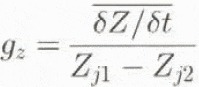
where Z j1 and Z j2 are the altitudes of the selected elevation intervals. From comparison of this gradient between glaciers in the same geographical area and with measured annual mass-balance gradients (b z), inferences about the emergence velocity (w s), and thus glacier dynamics, can be drawn (Etzelmüller and Sollid, 1996). If at a given location on the glacier δZ/δt < 0 and b z ≈ g zj then w s is low. If δZ/δt < 0 and b z g gz, then w s is high, and part of the mass loss is replaced by ice due to glacier flow. suggesting a more active glacier. On glaciers where a surge occurs during the measurement period, g z 0.
The change in slope combined with elevation changes indicates changes in driving stress. For example, a steepening of part or all of the glacier surface combined with only low surface elevation changes or even an increase in elevation in specific areas will increase driving stresses. This situation is often observed on surge-type glaciers during the quiescent phase (cf. Liestøl, 1969).
The change in curvature or local topography also provides information about changing flow behaviour. Plan curvature, which displays the curviness of glacier surface contours, is useful as a measure of magnitude and change of emergence velocities (w s). In the ablation area (+ w s) convex plan curvature and in the accumulation area (— w s) concave plan curvature are expected. The walls and floor of U-shaped valleys filled by a glacier have concave slope forms. A low-dynamic glacier in a downwasting stage will, with time, acquire a topography closer to the subglacial relief. The surface topography in this situation is expected to develop towards a more concave surface, especially in the ablation area. Therefore, high rates of change in surface topography during a period of surface lowering indicate an accentuated mirroring of subglacial relief on the glacier surface. Small changes in surface topography despite high surface lowering rates suggest that such glaciers maintain high flow velocities, counteracting mass losses by high ice flux.
2.3. Error propagation and strategies to quantify long-term changes of relief parameters over time
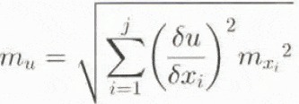
Succesful quantification of glacier surface change depends on the DEM quality and the degree of derivation of the DEM. The changes can be quantified through either arithmetical or statistical operations. Errors from the original data, sources propagate through these operations and normally increase (cf. Burrough, 1986). Given an arithmetical relationship
with x j being different information layers, the mean error of u for independent x j is
For correlated x j, Equation (3) is rewritten as
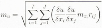
where m is the mean error and r ij is the correlation coefficient between two information layers.
2.3.1. Arithmetical operations The most straightforward way to quantify surface changes is by means of differential surfaces, which directly compare single relief parameter grids from different time steps simply by calculating the difference between two matrixes on a cell-by-cell basis (cf. Etzelmüller and Sollid, 1996). If u = x – y, the error propagates, following Equation (4):
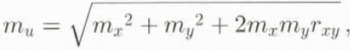
r xy being the correlation between the layers x and y. When the differences become small, the relative error increases. Consequently, the DEMs have to be of good quality and the mean errors have to be known and as small as possible. When r xy = 1, the mean error of the differential surface approaches the sum of the mean errors of the original data source. For high-quality elevation models the errors may be acceptable. With derivation of the altitude matrix, however, the problem with data noise increases. For example, slope is normally derived from the DEM by maximizing the gradient in the x and y directions in a local neighbourhood. The gradient is then calculated from the difference between two cell locations over the resolution K:u = 2K –1 (x – y). This results in the same error addition as shown in Equation (5). The error is, however, reduced with the factor 2K –1, showing that the error increases with decreasing cell size. Anyway, subtracting two noisy data sets gives weak results with high relative errors. This effect can be reduced by filtering the original data source or by calculating averages of the relief parameters in altitude intervals. The mean error within each interval can then be derived from the standard errors of the estimate of the mean (S e):
where σ is the estimate of the standard deviation and n is the sample size within the interval.
2.3.2. Statistical operations An alternative method is to calculate the correlation coefficient over the whole surface or in a local neighbourhood (local correlation). This results in a sort of statistical magnitude of change. Local statistical descriptors can be calculated by means of a moving window operation, applying: cov (B l, B 2)x,y =
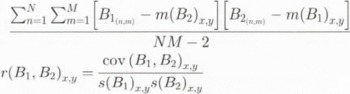
where m(B 1)i.j is the mean value in the window kernel with size N x M at the grid location of the surface B 1xy , s(B 1) i.j 2 is the standard deviation, cov(B 1, B 2)i.j is the covariance, and r(B 1, B 2)i,j is the correlation coefficient between the grid surfaces B 1 and B 2. The size of the moving window can be adjusted. A correlation coefficient close to + 1 indicates small changes of local topography, while a near-zero or even negative coefficient shows large changes.
3 Comparison Of Selected Spitsbergen Valley Glaciers Based On Relief Parameter Analysis
3.1. Introduction and settings
The aim of this comparison was to investigate how the surface change of Spitsbergen glaciers is represented by the geomorphometric measures. Five glaciers have been chosen (Fig. 1), where good quality DEMs from several years are available.
Erikbreen and Finsterwalderbreen are valley glaciers located in northwestern and southwestern Spitsbergen, respectively (Fig. 1). The thermal regime of both glaciers is polythermal, with a cold upper layer in the ablation area and in parts of the accumulation area (Ødegård and others 1992, 1997). Erikbreen does not seem to be building up to a surge at present because of the high velocities and mass fluxes measured, in relation to the other glaciers studied (Etzelmüller and others, 1993). Finsterwalderbreen surged at the turn of the 19th century (Liestøl, 1969).
Austre and Vestre Brøggerbreen and Vestre Lovénbreen are valley glaciers south of Ny-Ålesund on Brøggerhalvøya.
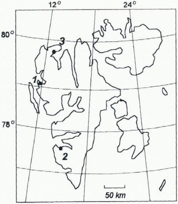
Fig. 1. Key map over Svalbard, with the glaciers investigated marked with black circles: 1, Austre Brøggerbreen, Vestre Brøggerbreen and Vestre Lovénbreen: 2, Finsterwalderbreen: 3, Erikbreen.
Austre Brøggerbreen is mainly cold-based, but borehole measurements indicate that paris of the base are at the pressure-melting point (Björnsson and others, 1996). Vestre Brøggerbreen and Vestre Lovénbreen are thinner than Austre Brøggerbreen (Hagen and others, 1993), and so presumably are mainly cold-based. These glaciers also had their maximum extent at the turn of the 19th century, which Liestöl (1988) presumes was due to surge advances.
3.2. Methods and accuracies
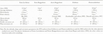
The DEMs of the glacier surfaces were constructed by different instruments based on air photos with varying scale. This resulted in varying accuracies (table 1), but relative accuracies within the DEMs were within 2 m and sometimes better than 1 m in the z direction. Absolute accuracies were calculated by comparison of field-surveyed points, revealing accuracies better than 2 m (Etzelmüller, 1995). If the original data were contours, gridding was carried out following Hutchinson’s (1989) procedure. To reduce errors, the grids were resampled to 25 m for altitude and slope analysis, and 50 m for curvature analysis, by bilinear interpolation. For calculation of the relief parameters, the method described by Zevenbergen and Thorne (1987) was applied, fitting a nine-term polynomial to a moving 3 x 3 window. Relief parameters are then calculated by derivation of the polynomial equation. All spatial calculations were done in ARC/INFO-GRID (© ESRI), and statistical analyses were performed with SAS and LOTUS 1-2-3 spreadsheets.
Accuracies of the surface change calculations were estimated using Equations (5) and (6). Absolute errors of the surface elevation change in single cell locations were less than 3 m (Table 1; Equation (5)), on Erikbreen as low as 1 m. However, errors in relation to elevation change (relative errors) are high close to the equilibrium line and in the accumulation areas with small surface changes. Within these accuracies cell values of slope cannot be compared directly on a cell-by-cell basis. Therefore, slope and altitude changes were averaged within altitude intervals, and standard errors of the mean were estimated according to Equation (6). For both Erikbreen and Finsterwalderbreen the errors do not exceed 0.5 m, which gives relative errors of less than 10% outside the ELA area. The errors of the slope change were on the order of 0.005∘ a–1, which gives relative errors of less than 10% for Finsterwalderbreen. For Erikbreen the errors were on the order of 0.007∘, a–1, which results in higher relative errors where average slope changes approach zero. On the smaller glaciers Vestre Lovénbreen and Vestre Brøggerbreen with basic accuracies around 2 m, even averaged values of slope may be critical because of the low number of cells in each altitude interval for the chosen DEM resolution. In these cases, only averaging over the whole glacier surface or statistical operations give reliable results.
3.3. Results and discussion
The hypsographic distribution of glacier surfaces is described by the altitude skewness and altitude median. Erikbreen showed negative altitude skewness (< – 1) and high altitude median values which reflect large areas at high altitudes. The other glaciers showed considerably lower skewness values, indicating a more even elevation distribution (Fig. 2a).
The long-term mass balance (b n) shows a high net mass
Table 1. Generation method and accuracies of the DEMs used
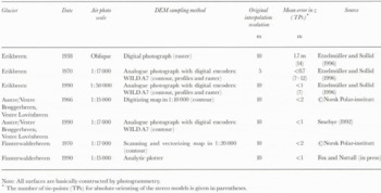
Table 2. Descriptive parameters for the glaciers investigated
loss for all glaciers except Finsterwalderbreen and the 1938–70 period for Erikbreen (Fig. 2b). The change in mean altitude was less than the change in median altitude, generally leading to a decrease of altitude skewness with time. This pattern was less accentuated on Erikbreen and Vestre Brøggerbreen (Fig. 2c). The magnitude of surface lowering in the accumulation area was higher on Erikbreen than on the other glaciers, while in the ablation area Erikbreen showed lower mass losses (Fig. 3). This is also displayed in the calculated gradients of surface elevation change (Equation (1)) which show smaller gradients for Erikbreen (>–0.15 m per 100 m a–1) in relation to Finsterwalderbreen and the glaciers on Brøggerhalvøya (>–0.25 m per 100 m a–1) (Figs 2b and 3). The field-measured annual net mass-balance gradients for glaciers in Spitsbergen is on the order of 0.3 m per 100 m a–1 (Etzelmüller and Sollid, 1996; personal communication from J. O. Hagen, 1996). On Erikbreen the gradient of surface elevation changes is less than half of this value, while on the other glaciers investigated the two gradients closely resembled each other, revealing higher mass compensation by glacier flow for Erikbreen. Finsterwalderbreen showed a clear increase in surface elevation in the accumulation area (Fig. 3), while the glaciers on Brøggerhalvøya showed a weak lowering or stationary situation (Etzelmüller and Sollid, 1996).
Slope and surface curvature are related to glacier thickness, which results in decreasing slope and curvature with increasing glacier thickness (cf. Paterson, 1994) and area. The standard deviation of profile curvature is higher than the standard deviation of plan curvature by a factor of around 1.5 for all glaciers studied (table 2), revealing the higher subglacial relief changes (e.g. riegels) in the direction of glacier flow.
Slope changes show a steepening for Finsterwalderbreen of >0.025° a–1 over the whole glacier, or a 10% change relative to the average slope. Erikbreen did not change, while the glaciers on Brøggerhalvøya showed a general steepening of 0.01–0.02° a–1 (Fig. 2d), or less than 5% of the
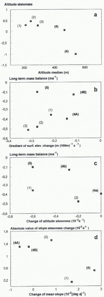
Fig. 2. Scatter plots of selected global topographic parameters and their changes for the glaciers investigated. (a) Altitude geometry. (b–d) Surface changes for the different glaciers. 1, Vestre Lovénbreen; 2, Vestre Brøggerbreen; 3, Austre Brøggerbreen; 4, Erikbreen; 5, Finsterwalderbreen.
average (table 2). Surface steepening in connection with a small change in slope skewness suggests that a glacier became steeper all over the surface, as observed for Finsterwalderbreen and Vestre Lovénbreen. On Erikbreen and Vestre Brøggerbreen the absolute slope skewness change was high (>0.013 a–1), indicating slope changes only in some parts of the glaciers (Figs 2d and 3). On Finsterwalderbreen the steepening of the surface is combined with an altitude increase (Fig. 3), implying an increase of driving stresses in time.
The change in curvature was quantified by local correlation analysis (Equation (7)). Both Finsterwalderbreen and Austre Brøggerbreen showed greater changes in the ablation
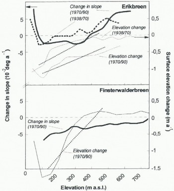
Fig. 3. Surface elevation change in relation to altitude and change in slope during the monitoring periods for Erikbreen (1938–70 and 1970–90) and Finsterwalderbreen (1970–90). Dotted line displays gradient of surface elevation change (Equation (1)). Negative values mean surface lowering. Change in surface slope is marked with thick line. Negative values denote a tendency to steeper slopes. Vales are averages, calculated in 50 m elevation zone. In contrast to Erikbreen, Finsterwalderbreen clearly showed surface altitude increase and steepening in the accumulation area.
area (lower local correlation coefficients) than Erikbreen (Fig. 4). The preservation of local topography in spite of the mass losses on Erikbreen is attributed to high glacier flow maintaining the surface profile topography (Fig. 4).
These results reflect differences between the glaciers which are attributable to glacier dynamics, in particular concerning the glacier’s possible surge behaviour during a period with retreat and mass losses. Although the sample size in this first study is too low to permit general conclusions, several parameters outlined above are useful for differentiating glacier types: On Erikbreen the change pattern of relief parameters (low slope change, flat gradient of elevation change, preservation of local relief) is interpreted to show that the glacier has maintained high mass fluxes during the measurement periods, preventing an increase of the accumulation area elevation. Negative altitude skewness values indicate that Erikbreen maintained high accumulation, which, however, is drained. Erikbreen therefore shows no clear sign of a surge build-up at present.
Finsterwalderbreen shows an opposite pattern to Erikbreen, with a general steepening of the surface and steep gradients of elevation change, indicating lower mass fluxes. Together with the elevation increase of the accumulation area, Finsterwalderbreen shows clear signs of building up to a surge.
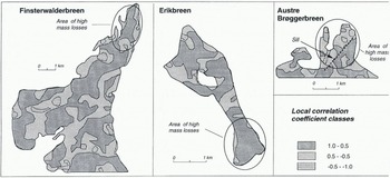
Fig. 4. Local correlation of plan curvature in a 20 year period. Erikbreen showed markedly lower changes in the ablation area than either Finsterwalderbreen or Austre Brøggerbreen.
The glaciers on Brøggerhalvøya showed a more comparable parameter pattern than Finsterwalderbreen concerning the altitude distributions and altitude change. Vestre Lovénbreen steepened over the whole surface area, while Vestre Brøggerbreen steepened only in some areas. However, on none of these glaciers was the increase in accumulation area elevation necessary for a surge build-up measured.
Parameters clearly distinguishing the three types of glaciers are altitude median and skewness (Fig. 2a). Erikbreen and Finsterwalderbreen differ in altitude skewness, while altitude median is of the same order. Finsterwalderbreen and the glaciers on Brøggerhalvøya differ only in altitude median. These glaciers seem to have surged (cf. Liestøl, 1988) at the turn of the 19th century, when the equilibrium-line altitude (ELA) was much lower. The present, increased ELA prevents them from surging.
4 Concluding Comments
The geomorphometric analysis reflects the different dynamics of the glaciers investigated in Spitsbergen. The method was tested on only a small number of glaciers, preventing general conclusions, but it is a suitable way of obtaining first impressions of changes in glaciers over time and in their dynamics based on aerial photography. The DEMs open the way to investigations of changes in surface form rather than just elevation changes, and the changes can be localized. The information obtained can be used to determine an earlier dynamical state of a glacier or as a first indication of glaciological characteristics of non-monitored glaciers. The parameterization of many glacier surfaces based on the techniques outlined opens the way to regional analysis of the distribution of different glacier types and their changes in time, based on single altitude statistics or indexes. Such an approach was introduced by Haeberli and Hoelzle (1995), who used a simple parameterization scheme for unmeasured glaciers to simulate potential climate-change effects on mountain glaciers.
The limiting factor consists in the availability of high-quality DEMs, If DEMs have to be constructed for the purpose of carrying out a geomorphometric analysis, including surveying of tie-points, etc., the effort and the results may not justify the costs, except for controlling mass-balance measurements. However, digital photogrammetry as an automatic tool is developing fast, and already allows cost-efficient DEM generation. Furthermore, national mapping agencies offer their topographic maps digitally, widening the availability of DEMs.
Acknowledgements
Digital photogrammetry analysis of the 1938 map of Erikbreen was carried out at Norsk Polarinstitutt, Oslo, by C. Rolstad. The digital 1970 map of Finsterwalderbreen was compiled by T. Tonning, based on a map from Norsk Polarinstitutt. The 1990 DEM was constructed by A. J. Fox of the British Antarctic Survey. J. O. Hagen and K. Melvold made Constructive comments on the study. The manuscript was much improved as a result of the critical reviews of R. Bindschadler and G. J. Young. Norsk Polarinstitutt gave permission to use their maps and air photos. The EU project on Finsterwalderbreen (grant EN5V-CT93-0299) provided the 1990 DEM of the glacier. The GIS work was entirely carried out at the Laboratory for Remote Sensing and GIS at the Department of Physical Geography, University of Oslo, Norway, as part of a Ph.D. project.


