


Introduction
According to a report by the International Centre for Integrated Mountain Development (ICIMOD), there are ~15 000 glaciers and 9000 glacial lakes in the Himalaya (Reference Mool, Bajracharya and ShresthaMool and others, 2005). These glaciers and glacial lakes supply fresh water to major river systems of the region, such as the Indus and the Ganges. Thus, their changes have significant scientific and socio-economic implications (Omura, 2006; Reference Key, Drinkwater and UkitaKey and others, 2007). A common view is that global warming gives rise to glacier retreat, resulting in expanding glacial lakes behind the newly exposed moraines, which are susceptible to sudden breach and consequent flood (Reference Bajracharya, Mool and ShresthaBajracharya and others, 2007). This type of event is referred to as a glacial lake outburst flood (GLOF) and occurs frequently enough in the Himalayan region to be of interest both to scientists and the public (e.g. Reference YamadaYamada, 1998; Reference Richardson and ReynoldsRichardson and Reynolds, 2000; Reference Mool, Wangda, Bajracharya, Kuzang, Gurung and JoshiMool and others, 2001a,Reference Mool, Bajracharya and Joshib). According to a study coordinated by ICIMOD, 44 glacial lakes in Nepal and Bhutan are potentially at risk of GLOFs (Reference Mool, Wangda, Bajracharya, Kuzang, Gurung and JoshiMool and others, 2001a,Reference Mool, Bajracharya and Joshib). This assessment was made with multiple criteria, such as a time history of the water level and conditions of the mother glacier and surrounding terrain, based on information gained from topography maps, photographs, satellite images and field surveys. Availability, high accuracy and continuous monitoring of topographic information are essential for successful evaluation of GLOFs and for understanding the underlying mechanisms (Reference Haeberli, Kääb, Mühll and TeysseireHaeberli and others, 2001; Reference Fujita, Suzuki, Nuimura and SakaiFujita and others, 2008).
The aim of this study is to update and improve glacier lake inventory for Bhutan, where a significant number of glacial lakes are located (2674 identified by ICIMOD; Reference Mool, Wangda, Bajracharya, Kuzang, Gurung and JoshiMool and others, 2001 a), using a new set of satellite data from the sensors on board the Advanced Land Observing Satellite (ALOS, ‘Daichi’ in Japanese). With their high spatial resolution and their efficacy in making digital surface models (DSMs), ALOS-based satellite data are particularly desirable for investigating glacial lakes. This study focuses on the various aspects of data-processing methods and presents preliminary results from the analysis of parameters of the inventory. Validation results are provided based on field observations taken at one of the potentially dangerous lakes listed by ICIMOD.
Data
ALOS was launched on 24 January 2006 and is currently in operation (Reference Shimada, Tadono and RosenqvistShimada and others, 2010). It has one radar and two optical instruments. This study uses images from the two optical sensors: the Panchromatic Remote-sensing Instrument for Stereo Mapping (PRISM) and the Advanced Visible and Near Infrared Radiometer type 2 (AVNIR-2). PRISM consists of three independent optical radiometers in the forward-, nadir- and backward-looking directions with a 2.5 m spatial resolution, which allow us to generate a DSM. PRISM-based DSMs have a height accuracy of 5–9m for different types of terrain including those in mountainous regions (Reference Takaku and TadonoTakaku and Tadono, 2009). AVNIR-2 is a visible and near-infrared radiometer with a 10m spatial resolution in the nadir direction. The calibration results of PRISM and AVNIR-2 and the validation result of DSMs generated by PRISM data have been reported by Reference Tadono, Shimada, Murakami and TakakuTadono and others (2009) and Reference Takaku and TadonoTakaku and Tadono (2009). So far we have used the best synchronous pair of AVNIR-2 and PRISM images from the period 2006–10 and continuously updating.
To validate basic parameters in the inventory, position measurements were taken at Metatshota lake (see Fig. 1 for location) with a differential GPS (ProMark3, Ashtech Co., Ltd). The post-data processing was performed using GNSS Solutions (Ashtech Co., Ltd). The key station for differential positioning was set at Gasa (27˚54.3' N, 89˚43.7' E) where continuous sampling for 40 days provided an accuracy of 0.37 and 1.07 m root mean square (RMS) for horizontal and vertical components in positioning, respectively. The relative positions and altitudes of the measurements were calculated on the Universal Transverse Mercator projection (UTM zone 45N and 46N in World Geodetic System 1984 ellipsoidal elevation (WGS84)).

Fig. 1. A mosaic image of the northern region of Bhutan constructed from ortho-images taken by AVNIR-2 over the period 2006–10. The locations of glacial lakes archived in our inventory are marked in yellow. The four sub-basins (Mo Chu, Pho Chu, Mangde Chu and Dangme Chu) are also indicated. The Metatshota lake area is denoted by a red box.
Data Processing
Starting with Level 1B1 images of PRISM and AVNIR-2, our data-processing procedure consists of four steps: orthorectification, geometric correction, pan-sharpening and digitization.
Orthorectification is a process used to correct topographic distortion that becomes serious towards the edges of each image. The distortion is sensor-specific and dependent on topography. Orthorectification of the PRISM images was performed simultaneously with the generation of DSMs using the DSM and Ortho-image Generation Software for ALOS PRISM (DOGS-AP), developed at the Japan Aerospace Exploration Agency (JAXA). For orthorectification of AVNIR-2 images, topographic information derived from an existing digital elevation model of the Shuttle Radar Topography Mission (SRTM) (Reference FarrFarr and others, 2007) was used with ground control points. The next step is geometric correction. Since the orthorectification removes distortions from both AVNIR-2 and PRISM images, the geometric correction here means co-registration of these images by means of tie points.
In the next step, pan-sharpening, we merge an AVNIR-2 image with lower geometric accuracy with a higher-accuracy PRISM image. This step is crucial for identifying and interpreting detailed ground features as required in making a lake inventory. We evaluated a class of pan-sharpening algorithms for one particularly suited to our study. Among the available algorithms, we first selected six: principal component analysis, multiplicative, the Brovey transformation, modified IHS (intensity–hue–saturation), high-pass filtering, and subtractive methods based on software availability (ERDAS, 2009). For the criteria of image quality, color balance, multi-band usage, and processing time, modified IHS and subtractive methods scored high. of these two algorithms, we finally selected the subtractive method.
The digitization step involves drawing a polygon for each glacial lake and storing it as vector data (shape files). When a lake is clearly visible and distinguished from the background (e.g. in a melted condition), its identification is straightforward. Unfortunately this is usually not the case for lakes in the Himalayan region. The melt season coincides with the summer monsoon, in which cloudy conditions persist and severely limit the number of clear images. To ensure that an object is a real lake, we sometimes run through the following quality-control procedure with the aid of DSMs: First, elevation contours are drawn over a pan-sharpened image. A simple test for a real lake is to see if the area is level. A more informative way of using DSMs is to draw an elevation profile. When in doubt we evaluate, for a lake candidate, elevation profiles in three cross sections, one in the longitudinal direction and two in the perpendicular direction. In many cases, we can identify lakes by examining those profiles (e.g. by the presence of end moraines). A difficulty in identifying lakes often arises from the presence of shadow zones. This problem is dealt with by looking at each pansharpened image in a panorama (bird’s-eye view) and sweeping it 360˚. This analysis provides additional terrain information about the locations of ridges and divides, and to a large extent eliminates false identification due to the presence of shadow zones. For less complicated cases we also utilize Google EarthTM in a similar manner. Although an attempt was made to use automatic and semi-automatic digitization algorithms, in the end we decided to work manually to utilize the maximum amount of topographic information gained from DSMs (see Reference PaulPaul and others, 2009).
Analysis
Lake selection
Numerous bodies of water exist in the mountain region. To screen for lakes clearly associated with glaciers, we set the following criteria. First we recognize that present-day terminal moraines in the Himalayan region were mostly formed by glacial advance during the Little Ice Age (LIA). For example, Reference Iwata, Narama and KarmaIwata and others (2002) concluded that the moraine for Raphstreng lake in the Lunana region of Bhutan was formed during the LIA and late Holocene. Glacial lakes in our definition are bodies of water that lie between the terminus of the mother glacier and the LIA moraine. Lakes located within 2 km of the LIA moraine down-valley are also included to take into account a possible flooding event involving multiple lakes. In addition, supraglacial lakes on debris-covered glaciers are included. Finally, we set 0.01 km2 as the minimum lake size, considering small lakes present less of a GLOF risk. Note that this differs from the ICIMOD convention, in which isolated lakes above 3500 m a.s.l. are listed as remnants of glacial lakes left due to the retreat of glaciers.
However, the parameters of our inventory mostly follow the ICIMOD convention, including ID, coordinates in terms of latitude and longitude of the lake center, area, elevation, width, length, and auxiliary information such as type of lake (e.g. moraine-dammed, etc.). Each lake has its own ID based on the name of the river sub-basin and latitude and longitude of the lake centre. In addition, we provide a cross-reference with respect to the ICIMOD code whenever available.
Validation and comparison with ICIMOD data
ICIMOD reported Metatshota lake, located in the Mangde Chu sub-basin, as one of 24 potentially dangerous glacial lakes in Bhutan that were at risk of GLOFs (see Fig. 1 for location). It is catalogued as Mangd_gl_106 in the ICIMOD report (Reference Mool, Wangda, Bajracharya, Kuzang, Gurung and JoshiMool and others, 2001 a). In September and October 2010, we conducted a field survey in the Metatshota area, taking GPS measurements. An ortho-image of the area from AVNIR-2 shows Metatshota lake and nearby smaller lakes (Fig. 2a). Unfortunately, there has not been a synchronous set of clear PRISM and AVNIR-2 images covering the area. For example, the best PRISM image so far for Metatshota lake is still partially covered with clouds. Figure 2b shows a pan-sharpened image over the area based on this non-synchronized PRISM and AVNIR-2 pair. With combined information available from these PRISM and AVNIR-2 images, we drew a polygon for Metatshota lake in yellow onto this AVNIR-2 image.

Fig. 2. (a) An AVNIR-2 image taken over the Metatshota lake area (data taken on 27 February 2010). The yellow polygons are drawn based on combined information from PRISM and AVNIR-2 images. The green curve is based on our GPS measurements overlaid on the AVNIR-2 image using their georeference. The red polygons are based on ICIMOD data (Reference Mool, Wangda, Bajracharya, Kuzang, Gurung and JoshiMool and others, 2001 a) overlaid on the same AVNIR-2 image. (b) A pan-sharpened image over the same area using a PRISM image from 3 October 2010. The upstream end of the shore of lake A is clearly visible.
The GPS position measurements were made along the shore of Metatshota lake. However, we could not make a complete circle around the lake due to the presence of steep terrain (see green line in Fig. 2a). To cope with this limit on the number of validation data, we first chose 44 of ~4500 GPS points with a nearly equal spacing. Then given each chosen point we computed a distance from the point to the nearest neighbor of the ALOS polygon. This quantity measures the accuracy of the polygon in the one-dimensional sense. The mean value of this quantity turned out to be 9.5 m, with a RMS of 11.7 m. These values can be taken as the first validation benchmark for our ALOS-based glacial lake inventory, although more work is needed to examine different sites for possible influences by varying terrain conditions. Currently we are waiting for clear PRISM images of the region to validate elevation data (DSMs) of the lakes.
We also overlaid a polygon based on the ICIMOD report in red. It can be seen that the ICIMOD polygon is significantly offset. The ICIMOD polygons were based on a series of topographic maps published in the 1950s–70s by Survey of India. Thus, part of the difference in lake size can be attributed to different observation times. However, the fact that the ICIMOD data show the location as significantly offset suggests that caution may be necessary when using them.
In Figure 2a there also appear smaller lakes (lakes A–C). Lake A is located down-valley of Metatshota lake. Our survey shows that there is a swamp area between the upstream shore of lake A and the moraine of Metatshota lake (Fig. 3). Our PRISM-based polygon for lake A clearly distinguishes it from the swamp area (Fig. 2). By comparison, the ICIMOD polygon for lake A appears to include this area as part of lake A. Again, this difference is likely attributed to different observation times. Overall, the above comparison shows that continuously improving and monitoring changes in glacial lakes with high-resolution satellite remote-sensing data is clearly necessary.

Fig. 3. Photograph of the Metatshota region showing Metatshota lake and lakes A–C.
Inventory
Construction of a glacial lake inventory for Bhutan is still underway. At present, the inventory covers >50% of the area and numbers 336 glacial lakes. This compares with the ICIMOD inventory listing 2674 glacial lakes, of which 562 are associated with glaciers. Figure 1 shows the locations of the glacial lakes in our inventory (marked in yellow). There are some data-void areas, due to the availability of synchronized cloud-free images of PRISM and AVNIR-2. In some mountain areas, cloudy conditions simply persist. To address this problem of data availability, we are moving towards using non-synchronized pairs, as shown in Figure 2.
Although the inventory is still in an interim state, we attempted to gain insights into the statistical properties of some topographic parameters of the inventory. In particular, we examined four sub-basins: Mo Chu, Pho Chu, Mangde Chu and Dangme Chu (see Fig. 1 for locations and Table 1 for summary statistics). Note that we include glacial lakes in China for the Dangme Chu sub-basin, as it runs through both China and Bhutan. So far, for these sub-basins we have counted 38, 117, 99 and 24 glacial lakes, respectively, accounting for ~80% of all the glacial lakes catalogued. The maximum lake sizes for the four sub-basins are 0.24, 1.38, 1.12 and 0.56 km2, with mean sizes of 0.07, 0.12, 0.06 and 0.10 km2, respectively.
Table 1. Summary statistics on glacial lakes in the four sub-basins

Figure 4a shows histograms of the lake count versus size classes for the four sub-basins. The size distribution is mostly dominated by small lakes (<0.05km2). However, the glacial lakes in Pho Chu have another peak in the range 0.1–0.5 km2. About 55% of the glacial lakes in the four sub-basins are <0.05km2 but these cover only about 13% of the area. Six of the largest lakes (>0.5km2), including Metatshota lake, account for ~20% of the total area. Figure 4b illustrates the distribution of lake elevation, which ranges between 4000 and 5500m a.s.l. The minimum elevation of the Mangde Chu sub-basin is the highest among the four sub-basins at ~4800ma.s.l., whereas the maximum elevation exceeds 5000ma.s.l. for all four sub-basins. The Pho Chu sub-basin again has double peaks at around 4500 and 5100m a.s.l.
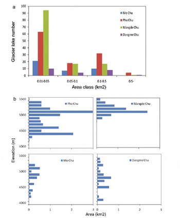
Fig. 4. (a) Glacial lake count versus size class for the four sub-basins. (b) Elevation intervals versus area covered.
Conclusions
The present study investigates glacial lakes in Bhutan. We have looked for a proper methodology to construct a glacial lake inventory based on newly available high-resolution PRISM and AVNIR-2 data from ALOS. The adopted procedure consists of orthorectification, geometrical correction and pan-sharpening steps before manual digitization. For Metatshota, one of the glacial lakes listed as a high GLOF risk, the field observations provide a validation estimate of 9.5 m for the location of the ALOS-based polygon, with a RMS of 11.7 m, setting a benchmark for the accuracy of this inventory. The analysis of the lakes in the four sub-basins reveals that the frequency distribution of lake sizes biases towards smaller lakes. Combining all four sub-basins, the smaller lakes (<0.05km2) account for ~55% of the total number of lakes and occupy 13% of the total area. Our results reiterate the abundance of small glacial lakes in Bhutan and rapid changes in geographical environments as seen in Metatshota lake. These results indicate the importance of implementing high-resolution satellite remote-sensing data, such as those by ALOS, to study glacial lakes. Currently we are working towards the completion of the glacial lake inventory as well as a glacier inventory of Bhutan. The sample version of our glacial inventory has already been released into the public domain. We plan to release the full version by the spring of 2012.
Acknowledgements
This work is carried out for the ‘Study on Glacial Lake Outburst Floods in the Bhutan Himalayas’ project under the Science and Technology Research Partnership for Sustainable Development (SATREPS) supported by the Japan Science and Technology Agency (JST) and the Japan International Cooperation Agency (JICA). We are grateful for support from the Bhutan Government and JAXA. Our special thanks go to J. Komori and S. Yamaguchi for their assistance during the field survey.


