


1. Introduction
Glacier retreat is a global phenomenon and since the 1990s, it is very likely caused by the warming of the atmosphere due to human activities (IPCC, 2021). On the three largest Icelandic glaciers, the equilibrium line altitude has risen by more than 200 m since 1973 (Hauser and Schmitt, Reference Hauser and Schmitt2021). In the period 1890–2019, the volume of Icelandic glaciers was reduced by 16% to ~3400 km3 (Aðalgeirsdóttir and others, Reference Aðalgeirsdóttir2020). The funeral of Okjökull as the first renowned Icelandic glacier that became a victim to climate change was a worldwide recognized media event (Bruns, Reference Bruns, Bødker and Morris2021).
In polar and subpolar regions, glaciers are often dome-shaped ice masses with radial flow, known as ice caps. Usually, such ice caps are large and cover the underlying topography. Direct mass-balance observations, which are based on in situ measurements of accumulation and ablation on the surface, can be hard to apply on such glaciers due to their large size and complex spatial variations in the accumulation and ablation fields. For this reason, the method of choice to study the mass balance of these glaciers is often the geodetic mass-balance determination, which converts distributed elevation changes into mass changes, assuming a mean density for the determined volume differences. Since elevation surveying techniques are either too expensive or too inaccurate for annual application, this method is commonly used over several years or even decades.
On Sléttjökull, the existence of an englacial tephra layer from the Katla eruption in 1918 offers a rare, but interesting opportunity to derive local mass-balance information from remotely sensed shifts of the layer outcrop. If the angle between the tephra layer and the ice surface along the flow is known, the apparent horizontal displacement of the outcrop in the ablation area of the glacier depends on the interplay of ice movement and ablation. The ice movement can be determined from ground observations or from remote-sensing data, which allows the calculation of the local surface ablation from the horizontal shift of the outcrop and the dipping angle of the ash layer. This approach is described by Mayer and others (Reference Mayer2017), who measured the dipping angle of the 1918 tephra layer along a crevasse and applied the model for the period 1988–2014. Here, we extend the methodology by a more extensive ground-penetrating radar (GPR) sounding of the tephra layer depth, which allows us to derive a 3D-model of this layer by interpolation of tephra depths between the GPR tracks. This enables us to calculate the apparent horizontal shift of the layer at several locations along the outcrop. We determined the apparent horizontal shift of the tephra layer in the direction of the local ice flow and combined it with the interpolated ash layer inclination, in order to minimize geometric errors in the original approach. By choosing four locations across the Sléttjökull outlet glacier lobe, we obtained more distributed information about the local mass balance. Based on a longer time series of satellite images, we could extend the observation period to 1988–2020.
2. Site description
The plateau glaciers Vatnajökull (7720 km2), Langjökull (836 km2), Hofsjökull (810 km2), Mýrdalsjökull (520 km2) and Drangajökull (137 km2), together with smaller glaciers, covered an area of 10.371 km2 in the year 2000, equivalent to 10% of the entire area of the island (Fig. 1) (Hannesdóttir and others, Reference Hannesdóttir2020).
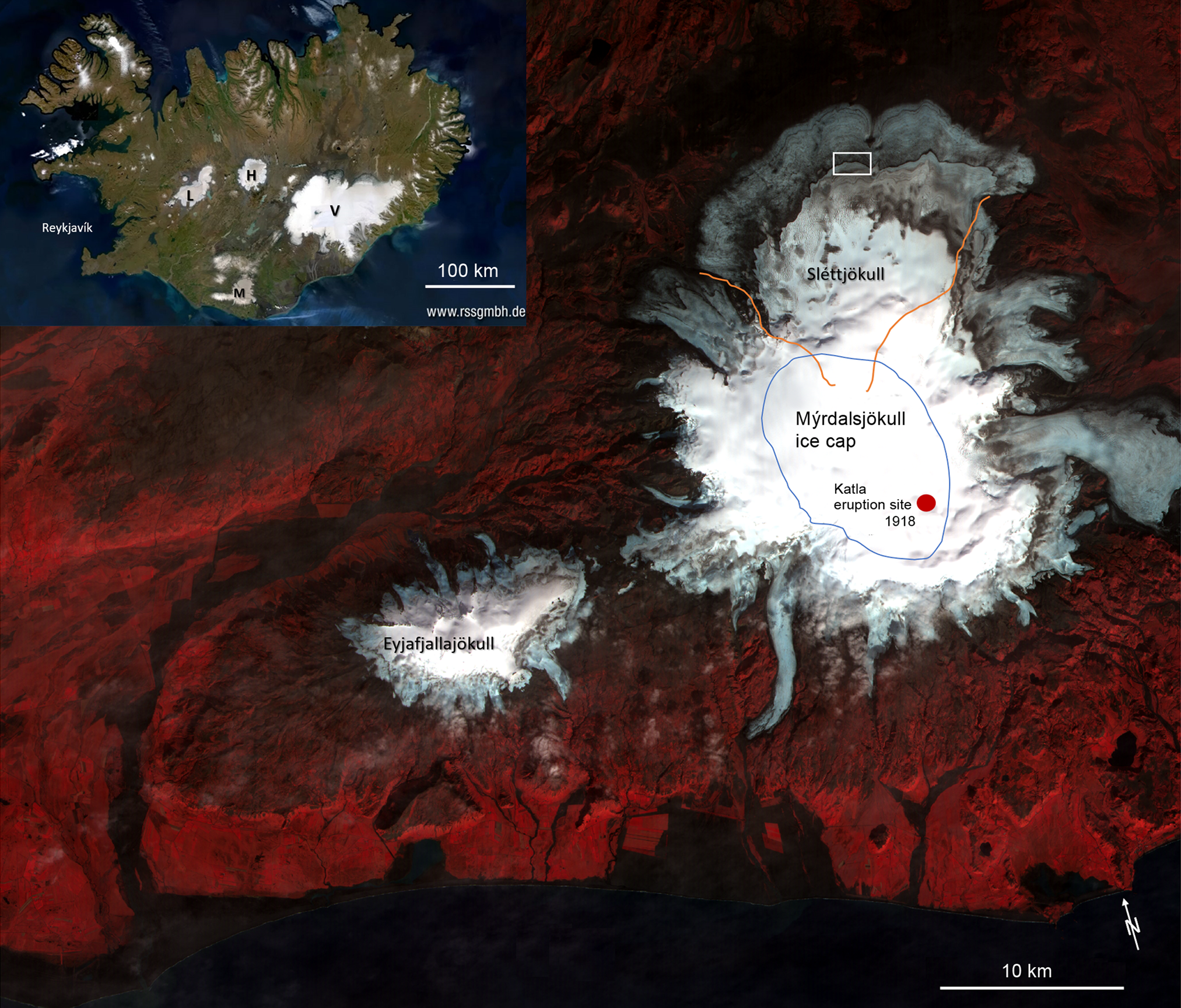
Fig. 1. ASTER false-color composite (red, green and blue, bands 3, 2 and 1) from 23 September 2004. The white square is the study area, the blue line represents the margin of the Katla caldera. Upper left: RapidEye mosaic of Iceland showing the main glaciers. V, Vatnajökull; M, Mýrdalsjökull; H, Hofsjökull; L, Langjökull; D, Drangajökull (© Planet Labs GmbH, ID RESA/DLR 619).
Mýrdalsjökull, located in the southern part of Iceland, is the fourth largest ice cap with a volume of 140 km3 (Björnsson and others, Reference Björnsson, Pálsson and Guðmundsson2000). The ice cap covers the Katla volcano and reached its maximum postglacial extent around 1890 (Sigurðsson, Reference Sigurðsson, Schomacker, Krüger and Kjær2010). Between 2000 and 2019, Mýrdalsjökull lost an area of 76 km2 (Hannesdóttir and others, Reference Hannesdóttir2020).
The ice cap extends over a height difference of ~1360 m, from 110 m a.s.l. at the terminus of the outlet glacier Sólheimajökull to the ice peak Goðabunga at 1495 m a.s.l. (Hansen and others, Reference Hansen, Jóhannesson, Sigurðsson and Einarsson2015). The morphology of Mýrdalsjökull can be divided into three areas: the center, which corresponds to the 130 km2 ice plateau of the Katla caldera; the northern lobe of Sléttjökull with an area of 157 km2; and the south, east and west steeply sloping outlet glaciers. The central area is characterized by 10–20 constantly changing ice depressions which illustrate the high geothermal activity of the subglacial Katla volcano (Björnsson and others, Reference Björnsson, Pálsson and Guðmundsson2000; Scharrer and others, Reference Scharrer, Mayer, Nagler, Münzer and Guðmundsson2007, Reference Scharrer, Spieler, Mayer and Münzer2008). The last subglacial eruption of Katla with catastrophic effects occurred in 1918 (Larsen, Reference Larsen2000), triggering an enormous jökulhlaup with estimated peak discharge values of 300 000 m3 s−1 (Tómasson, Reference Tómasson1996). Previous catastrophic eruptions occurred in 1625, 1660, 1721, 1755, 1823 and 1860 (Larsen, Reference Larsen2000). Mýrdalsjökull is characterized by both, high accumulation and high ablation rates. While accumulation can reach more than 7000 mm w.e. a−1, the annual mass balance on the plateau shows values between 2000 and ~6000 mm w.e. a−1 (Ágústsson and others, Reference Ágústsson, Hannesdóttir, Thorsteinsson, Pálsson and Oddsson2013). Ice melt is also highly variable across the ablation area, it reaches values of up to 10 m w.e. a−1 in the lowermost parts of the glacier (Þorsteinsson and others, Reference Þorsteinsson, Waddington, Matsuoka, Howat and Tulaczyk2005).
Katla erupted three times during the past century. The first eruption in 1918 produced massive pyroclastic fallout (Thordarson and Larsen, Reference Thordarson and Larsen2007). This tephra layer was buried in the accumulation area and has since then been transported and deformed by the ice movement. Radio-echo sounding in the central part of the ice cap detected the tephra in depths of 200–300 m, at the western rim of the caldera a maximum depth of even 460 m was observed (Magnússon and others, Reference Magnússon2021). The outcrop of the tephra layer is clearly visible on the glacier surface as a narrow black band on Sléttjökull (Fig. 2), where it is located at an elevation of ~900–1000 m a.s.l., which belongs to the ablation area in most years.

Fig. 2. Overview of the study area. (a) 3D visualization of the Sléttjökull catchment (blue line) based on UltraCam data from 15 September 2015. Contour lines at 50 m equidistance are based on the UltraCam DEM. The red line indicates the GPR profiles, white arrows point to the tephra outcrop. (b) Aerial photograph with the Katla tephra layer, 1918, view to the west, 16 August 2016. (c) View to the southeast, 29 August 2016 (Photos: U. Münzer).
The catchment area of Sléttjökull is characterized by radial ice flow and a smooth surface. The volume loss between 2014 and 2015 was calculated from UltraCam data, within the project IsViews (Iceland subglacial Volcanoes interdisciplinary early warning system) and amounts to 0.11 km3, or a mean elevation change of −0.7 m (Münzer and others, Reference Münzer, Eineder, Braun and Siegert2016).
3. Data and methods
3.1. Satellite imagery
The tephra outcrop was mapped on satellite imagery. For the year 2014, a Terra-SAR-X scene was used for this purpose and for the years 2015–2020, the task was achieved using optical satellite data. The years 2015 and 2016 were covered by Landsat scenes and from 2017 on, Sentinel 2 data were available. Table 1 gives an overview of these data. For 2021, cloud and snow cover prevented the use of images during the months which allow a comparison to other years (August, September).
Table 1. Date (YYYYMMDD), type and resolution of the used imagery

The surface slope, which is necessary for the determination of the dipping angle of the ash layer and for the delineation of flowlines, was derived from an UltraCam DEM. The UltraCam X large format digital aerial camera system is capable to shoot high-resolution images with high overlaps, which can be used to create accurate DEMs by digital photogrammetry (Gruber and Schneider, Reference Gruber and Schneider2007).
Very high-resolution UltraCam Xp data were acquired on 18 August 2014 and 15 September 2015. This camera was flown at an altitude of 3350 m above ground and 4000 m above ground, respectively, creating a sampling distance of ~20–25 cm. A total of 1804 (in 2014) and 453 (in 2015) stereo images were used to create DEMs and orthomosaics. The data were also used to calculate glacier velocities from feature tracking on the high-resolution orthophotos.
The UltraCam Xp images were processed with the software packages MATCH-AT (Trimble, 2022) and SURE (nFrames, 2022). Aerotriangulation (also known as bundle block adjustment) was also carried out using MATCH-AT (Albertz and Wiggenhagen, Reference Albertz and Wiggenhagen2009), for this purpose at least 20 tie points were identified per image. The co-registered (GPS) and inertial navigation system data were integrated into the aerotriangulation and hence the processing did not require any further ground control points. The semi-global-matching algorithm (Hirschmüller, Reference Hirschmüller and Fritsch2011; Heipke, Reference Heipke2017) was used to generate a dense point cloud from the oriented aerial imagery. The subsequent generation of the DEM and orthoimagery from the dense point cloud was carried out using SURE software.
3.2. GPR measurements
On 13 August 2016, more than 10 km of GPR tracks were recorded upstream of the 1918 tephra layer outcrop (Fig. 3). The GPR antenna was towed by a four-wheel drive vehicle (Fig. 4). The GPR equipment used was manufactured by IDS in Italy (RIS one) with a shielded bow-tie, dual-frequency antenna 200/600 MHz, in a plastic case.

Fig. 3. Location of GPR profiles on Sléttjökull. GPR 1–8: GPR data recorded on 13 August 2016 with intersection heights in meters a.s.l. B indicates the position of the base station. The basemap is the UltraCam true orthophoto from 18 August 2014, projected to the coordinate system UTM 27 N.

Fig. 4. Setup of the GPR measurements.
With a time window of 1.1 ns range and a sampling of 2.048 samples per trace, an approximate depth of 80 m can be reached with a vertical sample resolution of ~8 cm. Data used for tephra layer detection was collected with the 200 MHz antenna, while the 600 MHz antenna data were used for measurements of the firn depth. The acquisition rate was ~100 traces s−1, which translates to a horizontal trace spacing of ~1–3 cm, depending on the acquisition speed of ~1–3 m s−1, depending on surface conditions.
Planned transects were loaded to the onboard GNSS system of the vehicle allowing to measure predefined profiles. Due to difficult ice conditions, some of the predefined profiles were not covered. However, the location of the measured tracks was determined by post-processing of differential GNSS measurements (Fig. 3).
3.3. GPR processing
The GPR data were processed using the ReflexW software (https://www.sandmeier-geo.de/reflexw.html), by applying the following steps: (1) subtract-mean (dewow) to remove artificial instrument noise (wow noise), (2) move start time as a static correction in time, using the start time specified in the fileheader, (3) bandpass butterworth frequency filter to suppress noise with a frequency content other than the signal (works as a bandpass filter: for the 200 MHz data a low cut frequency of 100 MHz and a high cut frequency of 300 MHz was applied), (4) background removal to eliminate temporally consistent noise, (5) energy decay as a gain filter for amplifying the decreasing signal reflection strength with depth, (6) make equidistant traces by resampling the non-equidistant raw data in the space domain so the data become equidistant in the profile direction, (7) median xy-filter to suppress trace and time-dependent noise and spikes, (8) subtracting average as a filter to suppress horizontally coherent energy with the effect to amplify signals that vary laterally (e.g. diffractions).
For determining the real geometry of the tephra layer (Fig. 5) within the glacier ice the traces were corrected for the 3D topography of the ice cap. For transforming the two-way travel times of the GPR signal into depths, the wave velocity within the ice must be known. We assumed a constant velocity for ice of 0168 m ns−1 as commonly used for temperate ice in the literature (Eisen and others, Reference Eisen, Nixdorf, Wilhelms and Miller2002; Hubbard and Glasser, Reference Hubbard and Glasser2005).

Fig. 5. Radargramm of the profile GPR1 (see location in Fig. 3). The vertical scale was calculated with a wave velocity of 0.168 m ns−1. Surface elevation is taken from the corresponding GNSS profiles. A topography correction by vertical adjustment was applied to show the true englacial elevation.
Nine GPR profiles across the internal ash layer could be successfully processed (see example in Fig. 5). The ash layer is clearly visible in almost all profiles, except where the depth of the tephra layer exceeded what could be registered within the recording time of 1.1 ns.
The depth of the tephra along the profiles was subtracted from the surface elevation derived from the GNSS measurements, resulting in the true elevation of the tephra layer. The data were interpolated by the multigrid interpolation procedure by Hutchinson and others (Reference Hutchinson, Xu and Stein2011) in order to create a 3D-model of the tephra layer. This allows us to determine the correct tephra layer depth along selected flowlines of the glacier and calculate the dipping angle. Four flowlines close to the trans-sectional GPR tracks were determined by following the largest mean surface slope, using the UltraCam DEM. In order to avoid local anomalies, the horizontal displacement of the tephra layer outcrop was observed and averaged along 200 m wide buffers, centered at the flowlines (Fig. 6).

Fig. 6. Mapped tephra layer outcrops over time and location of the four selected flowlines. The background is the Sentinel 2 image from 9 September 2019.
3.4. Ice velocity
UltraCam Xp orthoimages of 2014 and 2015 were used to perform manual feature tracking of individual tephra cones close to the profiles displayed in Figure 6. Stable cones, which did not show disturbances by lateral ash displacement due to meltwater flow, were selected for this purpose. The derived annual velocities for the period 2014–2015 were compared with results from feature tracking using Sentinel 1 radar images (Wuite and others, Reference Wuite, Libert, Nagler and Jóhanneson and2022).
3.5. Ablation model
The ablation model, which was described by Mayer and others (Reference Mayer2017), is expressed by Eqn (1).

where a i, ice ablation (m w.e. a−1); x d, horizontal tephra outcrop displacement (m a−1); U h, horizontal ice velocity (m a−1); α, angle between the ice surface and the tephra layer (rad); α s, surface slope (rad).
When the net balance is zero (i.e. no net surface melt), the migration of the tephra outcrop is equal to the horizontal ice velocity It is important to note that this approach can only quantify ablation, but not accumulation. If positive values result from Eqn (1), they arise from inaccurate measurements and cannot be regarded as accumulation values.
By applying a simple 1-D flowline model, Mayer and others (Reference Mayer2017) showed that the inclination of the 1918 tephra layer increases by ~0.02° a−1 at the outcrop region on Sléttjökull. Even though this slight adjustment of the layer inclination has only a minor influence on the estimated local ablation, we corrected the values for the individual budget years.
4. Results
The ice velocities derived from the UltraCam Xp images taken on 18 August 2014 and 15 September 2015 are 16 m a−1 at profile 1, 13 m a−1 at profile 2, 11 m a−1 at profile 3 and 8 m a−1 at profile 4. This decrease from west to east was also observed by Wuite and others (Reference Wuite, Libert, Nagler and Jóhanneson and2022), who derived ice-velocity fields by offset tracking. Their absolute values are somewhat lower and range from 15.1 to 3.8 m a−1 in the same budget year, but this difference can be explained by the fact that the time interval between the UltraCam images is one month longer and therefore include a longer period of higher summer velocities. The results are also in good agreement to the local displacement of 13.4 m a−1, measured close to profile 2 between 2013 and 2014 with high accuracy GNSS receivers (Mayer and others, Reference Mayer2017). Since the velocity dataset of (Wuite and others, Reference Wuite, Libert, Nagler and Jóhanneson and2022) corresponds well with our observations for the selected periods and provides annual data for the entire period of observation, we decided to use it as input for our ablation model.
In Figure 6, the mapped outcrop lines from 2014 to 2020 are shown on a Sentinel 2 image from 2019. The four flowline profiles are situated near the radar tracks, where the measurements of the depth of the tephra layer should be most accurate.
The position of the four profiles and the inclination angles of ice surface and tephra layer at these positions is listed in Table 2.
Table 2. Location of the four profiles and inclination of surface and tephra layer

Angles are presented in degrees (°).
a Note that the angle between ice surface and tephra layer increases by 0.02° a−1 due to temporal changes of the emergence angle (Mayer and others, 2017).
The shift of the ash outcrop in flowline direction was calculated from the shift of the mean UTM north coordinate of every year, using the azimuth angle of the flowline and simple trigonometry. The results are presented in Table 3.
Table 3. Horizontal shift of the tephra layer (in m) in direction of the flowline at four profiles

Positive values indicate a shift in flow direction (downwards), negative values indicate a shift up-glacier.
The measured displacements are then used to calculate the local ablation at the four profiles from Eqn (1). Figure 7 compares the results with in situ measurements for Hofsjökull, an ice cap located 130 km north of our investigation area. We used data of the Hofsjökull N glacier (WGMS, 2021), which has the same general exposition (N) as our test site and the measurement location is at a similar elevation.

Fig. 7. Calculated local mass-balance time series for Sléttjökull and observed mass balance at Hofsjökull N (data source: WGMS, 2021, updated, and earlier reports).
Errors involved are uncertainties in the surface slope of the glacier, the emergence angle of the tephra layer, the surface velocity and the displacement of the tephra layer. While the surface slope is known to a high degree of accuracy from the high-resolution DGM (better than 0.2° across a distance of some ice thicknesses, i.e. 1–2 km) it has also the least influence on the accuracy of the results. The knowledge of the emergence angle is crucial, because a variation of this angle by 0.5° results in an uncertainty of the ablation rate of ~17% for the typical values that occur at Sléttjökull. This is a reasonable uncertainty range, as the emergence angle needs to be known on a smaller scale, even though the tephra layer is very smooth in flow direction. The largest uncertainty originates from the determination of the outcrop displacement, due to the usage of remote-sensing imagery with a ground resolution of ~10 m only. Even for clustering several displacement measurements close to the profile, the accuracy of the displacement will not be better than a few meters. Therefore, the resulting ablation value is affected by an uncertainty of ~±0.5 m.
The complete time series since 1988 is composed of the already published data from 1988 to 2014 (Mayer and others, Reference Mayer2017) and the new results after 2015, where now four calculated lines emerge, representing the four profiles along the selected flowlines.
5. Discussion and conclusions
With the exception of the year 2017/18, there is a good agreement between our mass balances for Sléttjökull and the values at Hofsjökull N (Fig. 7). This is rather surprising, because we compare local mass balances with glacier-wide values at a distance of more than 100 km, which would explain an offset in the absolute values. It should be emphasized that the mass-balance series at Hofsjökull cannot be regarded as the ground truth for our mass-balance results at Sléttjökull. Instead, they are the only possibility to check the plausibility of our results, not in terms of absolute values, but in terms of year-to-year variations of the regional mass-balance signal. The striking zigzag shape in the Hofsjökull series since 2011 is also visible in our results. The years with negative values at Hofsjökull are also the ones which cause the most negative values in our model by showing very large displacements of the tephra outcrop. The positive year in 2011/12 is probably due to the early date of the 2012 image from mid-July, when the snow had just disappeared, and represents absent ablation, but not an accumulation value (Mayer at el., Reference Mayer2017).
The year 2017/18 shows a large deviation between observations at Hofsjökull (+0.48 m w.e.) and our mass-balance value at Sléttjökull (~−1.5 m w.e.). We observe a negative (upward) shift of the tephra layer by 33 m on average on the sentinel image in this period, which causes the strongly negative mass-balance value. The reasons for this mismatch, however, are not clear.
A sensitivity test of our model shows that the angles of the tephra layer and the surface slope are the most decisive values, while the ice velocity has very little effect on the results. A difference in the input values by ±15% can change the results by 30% for the surface slope, by 15% for the slope of the tephra layer and by 5% for the flow velocity. The fact that the two slopes can be derived quite accurately, by a high-resolution DEM and on-site GPR data, supports the validity of our results. At least the large deviation in 2017/18 cannot be explained by an underestimation of the ice velocity. Even if we set the ice movement to zero in this year, the model gives a mass balance of −1.4 m w.e. a−1.
The results of the four profiles show some scatter, which is probably linked to variations of the mass balance due to different exposition, accumulation conditions and elevation. However, the straightforwardness of the approach suggests that it is suitable to quantify the local surface mass balance. After the initial effort of a radio-echo sounding field campaign, the annual mass-balance situation can now be estimated quickly and easily by observing the vertical movement of the tephra layer from satellite imagery. Our approach is a novel way to determine the local mass balance over a larger representative area than traditional point measurements. The method is not affected by small-scale disturbances such as supraglacial melt channels or other topographic irregularities, which offers certain advantages over traditional stake readings. The 10 m raster of Sentinel 2 is relatively coarse for an annual applicability and the use of remote-sensing products with higher spatial resolution would certainly increase the accuracy. By its very nature, the approach is restricted to volcanic regions, where tephra is deposited on gently sloping, smooth glacier surfaces. There, it allows to determine the annual mass balance over several years after an initial GPR field campaign.
Acknowledgements
We thank the editor, Tómas Jóhannesson and two anonymous reviewers for their thoughtful comments and efforts towards improving our manuscript. This work was financially supported by the Munich University of Applied Sciences HM and the German Research Foundation (DFG) through the ‘Open Access Publishing’ program. The remote-sensing data used in this study were made available within the 3-year project IsViews (Iceland subglacial Volcanoes interdisciplinary early warning system), the funding by the Bavarian Ministry of Economic Affairs and Media, Energy and Technology (ID-20-8-3410.2-15-2012) and the Bavarian State Ministry of Sciences, Research and the Arts (Kz 1507 12032) is gratefully acknowledged. The team also thanks the Icelandic research center (Rannsóknamiðstöð Íslands) for granting fieldwork permits (2/2014; 13/2015; 12/2016 and 4/2017). Special thanks to the Icelandic rescue team (Björgunarsveitin Dagrenning from Hvolsvöllur and Björgunarsveitin Víkverji) and to Guðmundur Unnsteinsson, Reykjavík, for the field logistic support. Gratefully acknowledged are Ludwig Braun and Matthias Siebers, Bavarian Academy of Sciences and Humanities, for their participation in the fieldwork. Thanks to the company GeoFly for the flight campaign within the project IsViews and for the pre-processing of the UltraCam data, as well as to Juilson Jubanski, 3D Reality Maps GmbH, for the final processing of the UltraCam data and the production of orthophotos and DSM.


 Open access