


Introduction
The two gigantic West and East Antarctic ice sheets have been the main targets of the scientific community’s interest, as their future changes could bring about environmental changes with global ramifications. In the few areas that are not occupied by ice sheets, some small local glaciers can be found. Their limited size (which speeds up their reaction to climate change) and their coastal location (where the variations in temperature are greater and more rapidly evident) rates these glaciers as natural systems that are sensitive to, and significant indicators of, climatic change. These small ‘local’ or ‘alpine’ glaciers (Reference ChinnChinn, 1985a) flow from cirques and rarely reach the main valley floors, and the termini are ground-based. They are virtually completely isolated and independent of the inland ice sheet. Their mass balance is mainly controlled by sublimation, wind erosion and accumulation. The glaciers closer to the coast also undergo melting, and when the terminus is cliff-shaped they are affected by dry calving. However, the weight of the various processes involved in the overall balance is not easy to quantify. Thus, this study aims at determining the short-term variations of a local glacier and at quantifying the individual processes at work.
The best-known examples of ‘local’ glaciers in Antarctica are located in the Dry Valleys and were first observed by field parties during Scott’s and Shackleton’s expeditions. The earliest studies were conducted in Victoria Valley in 1960/61 (Reference Calkin and CraryCalkin, 1971), and mass-balance measurements commenced in 1969/70. The average mass-balance change for the 1970–75 period was –0.083 mw.e. Reference Calkin and CraryCalkin (1971) indicated very small variations for these glaciers, and precise determination of such changes requires detailed surveys (Reference ChinnChinn, 1980). However, Reference ChinnChinn (1998) found a slight recession to be the dominant trend for the ice-cliff fluctuations of these glaciers. This type of glacier is also widespread along the coast of northern Victoria Land. They were first described by Reference Chinn, Whitehouse and HöfleChinn and others (1989). Many are located not far from the Italian Research Station at Terra Nova Bay. They are all cold- and dry-based glaciers (mean annual temperature recorded at an automatic weather station near Terra Nova Station: –14˚C; average temperature for the warmest month, December: –1.5˚C, and for the coldest month, August: –22˚C).
Strandline Glacier: Previous Studies
Since the first Italian Antarctic Expedition (1985), many studies have been carried out on the local glaciers and in particular on Strandline Glacier, a significant example of a local glacier in northern Victoria Land owing to its morphological and dimensional features, its location and working processes. Strandline Glacier has been monitored continuously. It is a local, cold-based glacier located on the southern margin of Gerlache Inlet, Terra Nova Bay (Fig. 1). It was named Strandline by Reference ChinnChinn (1985b) to underscore its close relationship with Holocene raised beaches. The Strandline (74˚42'S, 164˚02'E) descends from 330 ma.s.l., covers about 0.47 km2 and terminates in a cliff that is 25–30m high and 130 m from the sea (Reference Baroni and OrombelliBaroni and Orombelli, 1988).
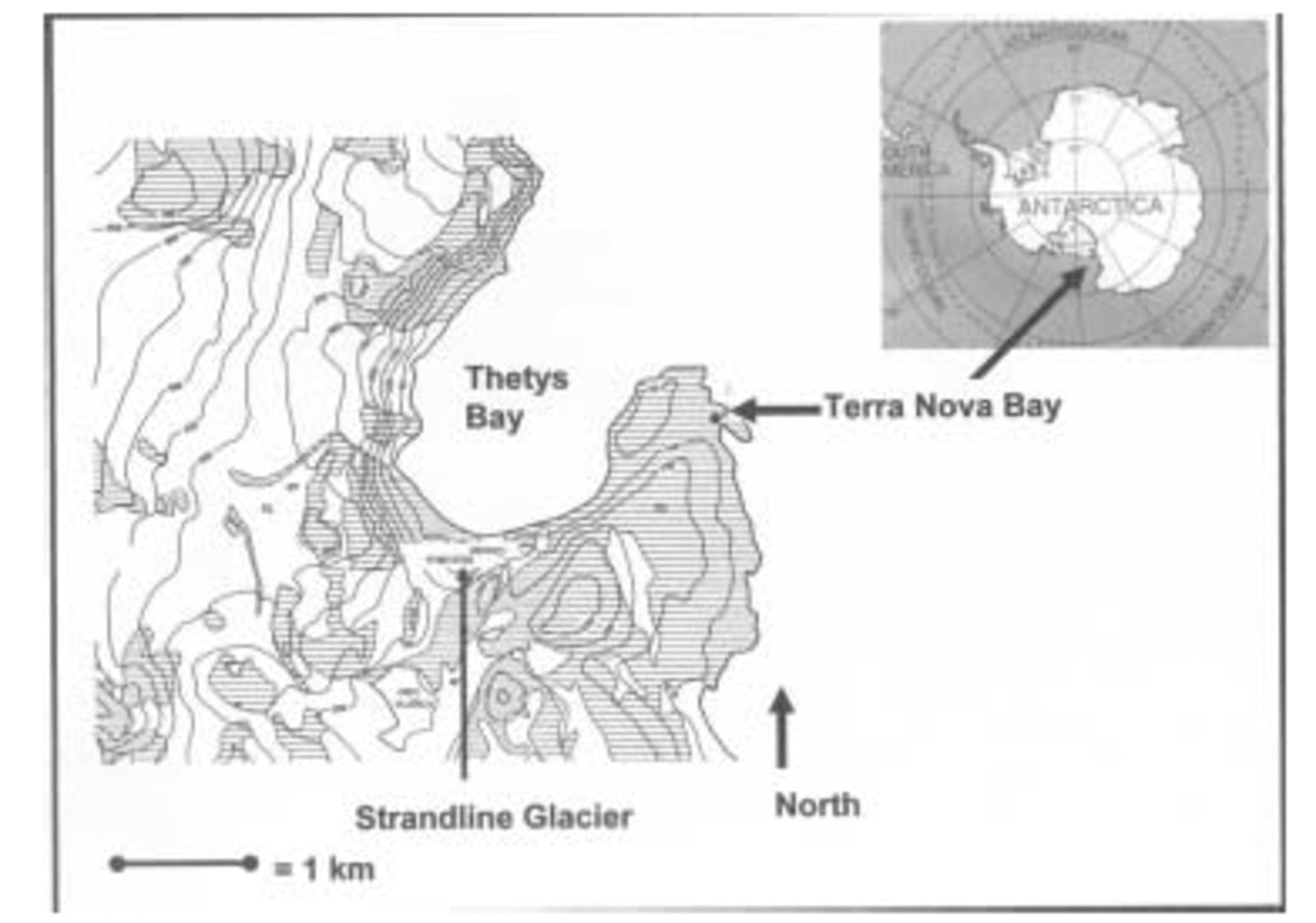
Fig. 1. Location map of Strandline Glacier. On the right side the arrow indicates the position of Terra Nova Bay, and on the left a second arrow indicates the same area on a zoom view of Thetys Bay where the glacier is located, close to the beach.
Since 1985, many methods have been adopted to assess the evolution of Strandline Glacier (Reference Meneghel and SmiragliaMeneghel and Smiraglia, 1991). Surface mass-balance variation measurements made using traditional glaciological methods (stakes) revealed a mean annual value of –0.017mw.e. (maximum of +0.110mw.e. in 1993, minimum of –0.007mw.e. in 1988) for the 1988–93 period (Baroni and others, 1995). Analytical photogrammetry has also yielded results of the same order of magnitude, and a comparison of the digital elevation models (DEMs) obtained from two aerial photograms (taken in 1956 and 1985) reveals a slightly negative trend (Reference Baroni, Frezzotti, Meneghel, Orombelli, Smiraglia and VittuariBaroni and others, 1995). Measurements of glacier terminus variations from fixed points beginning in 1987 show no significant variations, and any major changes appear to be related to local falls from the ice cliff (Reference Bondesan, Meneghel and SalvatoreBondesan and others, 2003).
Ice-thickness measurements by radio-echo sounding (RES) have been carried out on various sections of the glacier. The maximum ice thickness (about 80 m) occurs in the medium-low sector of the glacier (Reference Lozej and TabaccoLozej and Tabacco, 1993). Recent RES surveys performed during the 2002/03 National Italian Expedition have confirmed these results (Reference Motta and MottaM. Motta and others, unpublished information). Glacier surface velocity measurements have yielded mean values of 0.7–2.3ma–1 for the whole glacier over the period 1988–93. The central-western side of the glacier proved to have the fastest rate. Ice temperature measured at 10 m depth in a drillhole at about 82 ma.s.l. on the glacier surface was –14.3˚C (Reference RossiRossi, 1991).
Strandline Glacier: Recent Studies
During previous Antarctic expeditions, the largest mass variations observed on Strandline Glacier were near the ice cliff. The variations were not uniformly distributed throughout the Antarctic summer, but concentrated instead within a limited period of time. This time interval is characterized by higher air temperatures and greater exposure to sunlight. It was therefore decided to focus our study on a limited time period during the campaigns of 2000/01 and 2002/03, a time period during which, however, phenomena of greater intensity occur (according to the qualitative observations carried out during the previous Antarctic campaigns) and air temperatures are highest (according to the temperature data recorded at PNRA–Eneide meteorological station from 1987 to 1999; data by Programma Nazionale di Ricerche in Antartide (PNRA)–Ente per le Nuove tecnologie, l’Energia e l’Ambiente (ENEA)).
Measurement Methods and Results
To evaluate the overall short-term variations of Strandline Glacier, different approaches were needed in terms of the methods and techniques applied since the glacier is divided into two zones. The first zone, the glacier body, has a larger surface area and is easily accessible. The second zone, the ice-cliffed glacier terminus, is of smaller dimensions.
Studies carried out by Reference ChinnChinn (1985a Reference Chinn, b) for other local glaciers suggest that the driving processes, which cause short-term glacier variations, are not the same for ice cliffs and glacier surfaces. Therefore, the field surveys were focused on identifying and quantifying the driving processes that locally influence the glacier dynamics. Separate topographical and glaciological surveys for the two morphological zones were designed to quantify the variations and understand the working processes.
Topographical surveys
To quantify the area and thickness variations of the glacier, we decided to carry out a topographic survey using global positioning system (GPS) techniques. For the frontal ice cliff, we opted for a detailed total station survey to permit measurement of the vertical surface and quantification of the short-term variations of the profile. As a starting point for these procedures, several vertices with known coordinates were positioned near the glacier to improve the accuracy of the measurements taken by differential GPS Real Time Kinematics (RTK) with short bases. When used with short bases (<1 km), the positioning precision of this method is 1– 2 cm. The base GPS receiver was positioned on these fixed vertices. For this work, we positioned the base antenna receiver on metallic pegs on erratic blocks (located close to the glacier snout) instead of on the usual topographic tripod. This permitted greater stability of the base receiver (also under windy conditions) and thus also higher survey accuracy. The pegs have a 5/8 in (∼16 mm) upper thread for direct positioning of the GPS base receiver antenna. The antenna height was considered to be zero and it corresponded to the flush level of the fixed vertex peg when completely tightened. The local geoid undulation was estimated to be –57 m. The base reference station was located in vertex 100, at the bottom of the ice cliff on the glacier. Communication between the base and rover stations was managed by a Satel 3Asd radio-modem, with a frequency of 468.200 MHz. A signal amplifier was also used; it was located in the upper part of the glacier, for better coverage over the entire glacier surface of the signal transmitted by the radio-modem located in vertex 100.
Glacial body measurements
RTK GPS measurements were used twice during the same Antarctic expedition (at the beginning and end of the campaign) to quantify the changes that had taken place on the glacier surface and to lay the foundations for future surveys (Reference Rentsch, Welsch, Heipke and MillerRentsch and others, 1990). This method is ideal for accurate estimates of planoaltimetric variations (Reference Vassena, Diolaiuti, Motta and SmiragliaVassena and others, 2001). It also allows repeated measurements at the same point positions without using stakes to mark them on the glacier surface, thus making it possible to increase the number of measurement points. The first survey of Strandline Glacier was carried out at the beginning of December 2000. A total of 1020 planoaltimetric points (with an accuracy of 1–2 cm) were acquired along the entire surface of the glacier (each measurement point required a survey time of 15 s). A DEM (Fig. 2) was obtained after GPS data processing on the basis of a regular 10 m grid and by applying a kriging method to the survey data.

Fig. 2. DEM of Strandline Glacier. Both the positions of the stakes used for the mass-balance evaluation and the positions of the stakes located close to the ice-cliff boundary (used to calculate its erosion) are reported. In the lower part of the figure the two DEMs of the ice-cliff terminus processed by using data surveyed in December 2000 and in January 2001 are reported.
A second GPS survey was carried out near the end of the summer, and 100 points were selected from those surveyed the first time. Comparison of the two sets of points (equal to 10% of the first GPS survey data) revealed a quasi-stable situation, with variations of about the same magnitude as the instrumental accuracy (±0.05 m). The results do not show a clear division between the accumulation and ablation areas on the glacial body (Reference Vassena, Diolaiuti, Motta and SmiragliaVassena and others, 2001). The highest ablation was measured in the lower part of the glacier, where the surface indicates convexity shaped by eolic erosion.
Terminus measurements
To evaluate ice-cliff variations, taking into account the morphological features and the need to be informed of the changes in separate sectors of glacier terminus during the time interval, 13 vertical profiles were planned for two different periods. They were surveyed starting from 13 measurement points (identified 801–813) marked on the ground by cairns and mapped by GPS RTK techniques. Vertical profiles were surveyed using a total station GPS unit; the data obtained were processed and transformed into Universal Transverse Mercator (UTM) system coordinates. Totals of 252 points in the first survey, conducted on 22 December 2000, and 340 points in the second, conducted on 9 January 2001, were acquired. The choice of such a short survey period was based on the qualitative observations of the ice-cliff behavior during the previous expeditions. These observations indicated (Reference Motta, Diolaiuti, Vassena and SmiragliaMotta and others, 2003) substantial retreat of the ice cliff when meltwater is available and that this meltwater is present during a short period characterized by higher air temperatures.
For each survey, a three-dimensional model representing the ice-cliff surface and morphology was processed using Surfer 7 software. The model was obtained on the basis of a regular 1 m grid and calculated by applying a kriging method to the survey data. Comparison of the two DEMs permitted calculation of the volumetric change, which on a comparison surface of 4051 μ2 was equal to –351.53 m3. This value corresponds to a mean thickness loss of –0.087m over the entire vertical surface, with a mean daily value of –0.0048 m. These last two values represent a gross simplification, for it is assumed that the measured change was uniformly distributed spatially and temporally (Fig. 2, bottom). The ice-cliff surface used for the comparison was identified and blanked on the basis of the upper surveyed points (in the lower part of the profiles) and the lower points (at the top of the profiles). A blank of the data above 25m in altitude was used in order to exclude the apron area (which was surveyed by total station and was appreciable on the profiles obtained) from the processed data. The apron area does not permit a real three-dimensional reconstruction of the ice-cliff surface geometry. Detailed comparison of the 13 profiles surveyed at the beginning and the 13 surveyed at the end of the campaign led to the identification of various trends for the different ice-cliff sectors (Fig. 3). As can be noted in the planimetric view of the ice-cliff boundaries (Fig. 3, bottom), which were mapped using the data collected in December and January, the lateral zones, where the front morphology changes from an ice-cliff shape to a dome and a ramp shape, showed the smallest variations. The central sector showed the greatest variations, amounting to about 2 planimetric meters of retreat (Fig. 3, bottom). It is thus clear that the mean reduction (–0.087 m) calculated over the entire terminus surface is a result of the –2m change in the central sector (ice-cliff shaped) and of the variations amounting to a few centimeters or less in the lateral sectors (ramp- and dome-shaped).

Fig. 3. Profiles comparison. On the y axis the altitude values (in m) and on the x axis the distance (the north value in m) are reported. In the bottom panel, the ice-cliff boundaries for a planimetric comparison of changes between December and January are reported. The numbers (801–813) on the map indicate the position of the 13 points from which we measured the ice-cliff profiles; also marked on the map is the position of the fixed vertex 100 (used to calculate all the coordinates of the profiles’ data).
Glaciological measurements
Glacier body
A network of ten glaciological stakes was used to evaluate accumulation and ablation on the glacier body surface. Some pits were also dug in the upper zone of the glacier to study snow stratification. The surveys revealed that Strandline Glacier is characterized by accumulation zones where wind-borne snow accumulates and summer melting gives rise to very limited seepage. The presence of meltwater was demonstrated by stratigraphical surveys. Water accumulation and refreezing was observed in crevasses in the upper part of the glacier, along with the formation of veins of congelation ice (ρ ≈ 910 kg m–3). Ice of a different density (ρ ≈ 893 kg m–3) was observed enclosing the veins. This ice may be linked to metamorphic processes involving viscoplastic flow, in accordance with the rheologic zones of dry-based local Antarctic glaciers (Reference ChinnChinn, 1985a Reference Chinn, b). This ice deteriorates more rapidly when exposed to sunlight, particularly on the frontal ice cliff, and is characterized by a different albedo and density (ρ ≈ 706 kg m–3), similar to those of firn.
The thickness variations measured by field glaciological campaigns on the glacier body surface confirmed and validated the results calculated by the topographical GPS RTK surveys. The mean value obtained by stake measurements was –0.04mw.e.
Glacier terminus
Although in some zones (corresponding to vertices 806– 807–808 and to the sector identified by vertex 811 on the map in Figure 3), the field surveys made it possible to identify mass loss (in a range of meters) through calving, the limited variations in the lateral sectors were not linked to the same ablation processes. Therefore, further glaciological analyses (at the same time as the topographic survey) were carried out to identify the other processes responsible for the short-term variations on Strandline Glacier and to quantify energy transfers at the glacier–air interface.
During the 2000/01 and 2002/03 field surveys, 13 vertical stakes (Fig. 2) were located on the glacier surface close to the ice-cliff upper limit in order to calculate the daily erosion of the boundary. The data collected during the two campaigns showed that the erosion was not distributed homogeneously, and the main boundary changes (–2m of linear retreat of the boundary in the 2000/01 campaign and –4m in 2002/03) were concentrated in the zone around stakes 10–12 (also corresponding to vertices 806–807 and 808). The observations indicated that the ice losses were due mainly to falls of ice through dry calving processes. Thus, the glaciological surveys confirmed the data obtained from the topographical measurements at the ice cliff.
Not only dry calving but also melting and sublimation are ablation processes at work on the ice cliff and on the glacier surface. The evaluation of the energy and mass surface balance was carried out during the 2000/01 field campaign. During the 2002/03 campaign some experimental parcels were studied to define and quantify these processes. Parcels are glacier areas (parcel mean surface extension: 5 μ2) chosen from the glacial body or the lateral zones of the ice cliff at a location where calving is not present and the other processes have to be identified and quantified. The parcel boundaries were marked by expressly dug channels that intercept and divert the waters originating up-glacier, and by other channels that collect the meltwater produced inside the parcel. The first step was to quantify the mass loss for each parcel and to identify the driving processes.
Mass loss by evaporation and/or melting was measured by removing a block of material (ice and/or snow) from each parcel, weighing it and replacing it in its original position on the glacier in a plastic container of the same shape (Reference Motta, Diolaiuti, Vassena and SmiragliaMotta and others, 2003) without compacting the material. After a time interval (of hours and/or days), the block inside the plastic box was measured again in order to quantify the difference in weight brought about by ablation processes (melting and/or evaporation). To better understand which processes were responsible for the mass loss, we prepared two different sample boxes for two different blocks of the same material (ice and/or snow) taken from glacier areas close to each other in the same parcel. In one case, the block was inserted in a plastic box with small holes on the bottom so that the meltwater produced by the melting process would be lost, and we measured the overall mass loss (by evaporation and by melting). In the second case, the plastic box had no holes and all the meltwater remained inside. Therefore, only the mass loss due to evaporation processes was measured. The two sample boxes were positioned in the same parcel at the same time, so we could obtain the exact amount of melting and evaporation on those glacier areas
The next step was to quantify energy transfers at the glacier–air interface and the consequences for the mass loss. Particular attention was paid to the snout–ramp zone, where evidence of melting has been observed during previous field campaigns (corresponding to section 813 on the planimetric map in Fig. 3). For this purpose, the parcels were equipped with the following instruments:
1. Testostor 175 mini data logger programmed for executing synchronized temperature surveys at depths of 0.12 and 0 m every 2 min. A white cover shaded the probe at 0 m. The other probe was shaded by the box.
2. Box A, made of PET, was transparent, 0.12 m high, with an absorption coefficient of irradiance of 24.0 ± 0.5%. It was immersed in the ice and/or snow until its upper rim was flush with the glacier surface. It was filled with a block of material.
3. Box B, similar to box A, but the bottom was equipped with 1 mm diameter holes to allow meltwater drainage.
4. HD9071 data logger with LP9021RAD radiometric probes (spectral response 450–950 nm; calibration uncertainty <5%; mean cosine error <6%; non-linearity <1%) inside a horizontal tunnel protected from light penetration by means of a light-grey PVC pipe. The probes measured the downward and upward flux (Reference Liston, Winther, Bruland, Elvehøy and SandListon and others, 1999; Reference Biancotti, Motta and MottaBiancotti and others, 2000) at 0.12 m depth.
5. HD9021 data logger with LP9021UVA radiometric probes (spectral response 315–400 nm, error and set-up of the probes as with LP9021RAD).
6. Ablatometric stake made of light-grey PVC; albedo similar to the ice surface. Measurements were taken upstream, downstream and sideways, and then averaged.
The material in the boxes was weighed at intervals in order to quantify the losses and identify the processes at work. At the same time, albedo and the specific weight of the material in the box were also measured using the standard International Classification for Seasonal Snow on the Ground method, and then the block of material was repositioned in the box.
The main drawback of calculating the energy balance by box measurements is the impossibility of placing exactly the same starting mass inside the two boxes (due to the different specific weights). We therefore calculated the changes in mass taking into account the different starting weight of the material in the two boxes. The procedure is explained in the following example (using data collected on 5 December 2003). In box A (located on the lateral side of the terminus in the snout–ramp zone), we measured 20 g of mass loss. This was due to evaporation only, as box A (without holes) retains the meltwater produced. Applying a simple ratio, i.e. (weight of box A) : (loss by evaporation in A) = (weight of box B) : (loss by evaporation in B) (all measurements in g) for box B, we calculated that a mass of 17 g should have evaporated. In box B (with holes), the mass loss measured was instead 175 g (by both evaporation and melting). Considering the calculated 17 g of mass lost by the evaporation process, the meltwater produced must be equal to 158 g. This water value was used to calculate the amount of water produced in box A, which in proportion must be equal to 183 g. As the total quantity of water measured in box A was 160 g, it followed that 23 g must be trapped in the porosity of the material.
For the study period the mass balance obtained through the survey of the boxes was:
Melting of box A (with ρ = 0.64): 28.6 kg m–2
Melting of box B (with ρ = 0.55): 24.7 kg m–2
Evaporation of box A (with ρ = 0.64): 3.1 kg m–2
Evaporation of box B (with ρ = 0.55): 2.7 kg m–2
The energy balance was:
Net energy used for melting in box A: 334 kJ kg–1. 28.6 kg m–2 = 9552.4 kJm–2
Net energy used for melting in box B: 334 kJ kg–1 × 24.7 kg m–2 = 8250 kJ m–2
Net energy used for evaporation in box A: 2500 kJ kg–1 × 3.1 kg m–2 = 7750 kJ m–2
Net energy used for evaporation in box B: 2500 kJ kg–1 × 2.7 kg m–2 = 6750 kJ m–2
The balance (average of A and B) was 8901 kJ m–2 due to melting and 7250 kJ m–2 due to evaporation. The total energy exchanged by melting is a larger amount because the water inside the ice porosity freezes during the night, returning the melt energy absorbed.
Another way of evaluating the energy balance is by an indirect approach (we can adopt it if the quantity of irradiance absorbed by the glacial surface is known). With fair approximation (density slightly affects absorbed radiation; Reference Motta and MottaMotta and Motta, 2003), on a surface large enough to disregard the boundary conditions, the radiation absorbed by the boxes is equal to:
where R ass is the absorbed radiation, R i and R e are the incident and emitted radiation at the glacier surface, respectively, and D 12 and U 12 the downward and upward flux at 0.12 m depth (depth of box A). For a material like that contained in the two previously described boxes, having a constant thickness and which is large enough, the formula can be approximated to:
where I (irradiance) is the power absorbed by a square meter. D 12 and U 12 can be disregarded in first approximation; in fact, from the field data collected, D 12 is 1.5% of R i and U 12 is less than one-seventh of D12 (Fig. 4). This result means that the process developing in the boxes represents at least 98% of the melting process.

Fig. 4. Comparison of U 12 and D 12 data collected during the 2002/03 field campaign (in W m–2). U 12 is less than one-seventh of D 12; the line interpolates the measurement points.
While the boxes were left to work, the radiometers measured I. The energy absorbed in the same period as that of the previous example was as follows: visible and infrared 8350–18 140 kJ, ultraviolet 259–340 kJ according to the coalbedo used. Albedo ranged between 0.28 for the snow and 0.40 for the ice. So the energy balance was 8.6–18.5 MJ. These results can be compared with those yielded by the boxes, and the co-albedo increased in a way approximately proportional to density. Whichever measurement method was used, the absorption capacity of solar energy increases with density.
Finally we calculated melting and evaporation in relation to the superficial ablation, using ablation stakes. While the boxes were at work, the surface lowered by 0.025 m. According to the density of the shallow snow, this value corresponds to 11.2 kg m–2. Applying a ratio with the quantity evaporated and melted in box B, 1.09 kg m–2 proved to have evaporated and 9.48 kg m–2 melted. This value corresponds to an energy income of 5723 kJ m–2, which is definitely lower than the values calculated above through the box data. The explanation is that on the glacier surface, evaporation (and therefore energy absorption) measured by stakes was proportionally higher than in the top few centimeters of depth as measured by the boxes, and surface melting was lower because of the surface temperature conditions. In the field, we observed that on a warm day the glacier surface stayed below zero for <9 hours and that the length of this time interval decreased sharply with increasing depth, so that the time-span of temperatures below zero for 0.12m depth was <4 hours. The rate of temperature variations was calculated in the range of ±1˚Ch–1. The surface ice temperature measurements collected in the same field campaign showed strong daily fluctuations. A negative peak in the temperature values was measured at 0.12m depth when the surface temperature dropped below –6˚C. Otherwise at 0.12 m depth, the ice remained constant at the melting point. Melting is therefore a very important ablation factor. Within the same period, it varied from 13.3 ×10⁻⁶ to 181.4×10⁻⁶ kg m–2 s–1. These variations could be caused by wind (greater evaporation) and cloud cover. In Figure 5, a diagram of the energy balance of a parcel in the ramp zone is reported. The air temperature remained slightly below 0˚C for the entire measurement period (1 week during summer 2000/01).

Fig. 5. Energy balance of the parcel in the ramp zone at the terminus of Strandline Glacier during a week of measurements in summer 2000/01. Time (daily hours) is reported on the x axis, and energy (Wm–2) on the y axis.
Discussion
The Strandline Glacier data indicate that the variations of the glacier during the Antarctic summer are due to various processes that are active in different glacier sectors. The actual glacial body (without considering the ice cliff) is influenced on the surface by wind action, which removes material and sets it down again locally. A further effect of the wind is to increase the evaporation and to lower surface temperature, causing a decrease in the melt rate. This contributes to keeping the short-term glacier surface variations within a very limited range. Melting and sublimation processes are surely active as well. The amount of melting in summer is greater than that caused by sublimation processes (according to the data obtained from the two experimental parcels) and it increases with depth for the temperature conditions. The meltwater produced does not stream down the glacier and/or ice-cliff surface. It was produced in a subsurface layer (from our experiments at >0.1m depth) where temperature conditions are constantly close to the melting point. Here a small amount of meltwater fills the air pockets within the material (snow and/or ice) and so it is not lost. The other, larger amount of meltwater follows a different path according to the two glacier zones: (i) on the glacier body, where, as verified by pits dug during the 16th Italian Antarctic Campaign, it refreezes developing veins of congelation ice; and (ii) at the glacier terminus from where it flows through sub-superficial channels to the bottom of the apron, through which it is lost.
The frontal ice cliff presented the greatest volumetric variations of the entire glacier and this surely has a strong impact on the mass balance of Strandline Glacier. Some ice-cliff sectors, corresponding to the direction of the glacier’s main flux line, showed a loss of about 2 planimetric meters during the 2000/01 survey, and about 4 planimetric meters during the 2002/03 survey, due to dry calving processes, whereas the lateral ice-cliff sectors showed smaller losses caused by different processes. The experiments performed in the parcels permit us to underscore how active melting and sublimation are here (as on the glacier body surface) and the important role played by melting. However, it is not easy to define this role since meltwaters take some time to flow down from the glacier. Moreover, meltwaters on the ice cliff, unlike those on the glacier body surface, represent a real loss of material since there is no water regelation and they are discharged from the glacier through sources at the bottom of the apron. The difference in the behavior of the ice cliff is also linked to the specificity of its geometric and dynamic features, compared to the other glacier zones, and, consequently, to the difference in albedo and irradiance, which change the glacier energy response here. The influence of the calving processes on the variations in the mass of this local Antarctic glacier was an interesting aspect of this research. Profile 807 in the central part of the ice cliff (Fig. 3) is of particular interest, as it revealed a sector projecting and jutting out in the uppermost part of the ice wall during the first survey, only to then leave behind a reentrant wall in the second survey. This is the central part of the terminus, where the flow rate is higher (2–3m a–1). Here, on the top of the ice cliff, the formation of longitudinal crevasses was initially directly observed. Then later, the crevasses were found to propagate downward and an overhang had developed. Some calving of slabs from the ice wall was directly observed with the rotation of the cliff profile prior to the failure. Therefore, it can be stated that ablation in the central sector of the glacier front is prevalently due to dry calving processes.
Given that the greatest variations take place in the summer and that the summer is marked by the presence of melting processes, it can be deduced that meltwater must play a role of some importance. These waters are produced and released in the lower part of the glacier and may play a dual role: (a) increasing the mass weighing upon the unstable blocks of ice (during the measurement campaigns, crevasses filled flush to ground level were often observed in the frontal sector); (b) lubricating movements of the unstable blocks.
Conclusions
The Strandline is a small, cold-based, ice-cliffed glacier: a good example of the local ‘alpine’ glaciers of northern Victoria Land. Repeated monitoring campaigns revealed slightly negative variations in thickness, suggesting a situation close to a steady state or possible minor recession. The joint use of different analysis methods permitted the detailed study of active ablation phenomena and a better understanding of their driving processes.
The summer survey campaigns permitted us to quantify variations in the mass and on the front of the glacier. A comparison of these variations with the annual variations allows us to state that the most substantial changes take place during the summer (approximately –2 planimetric meters at some isolated points of the ice cliff in 2000/01). Thus changes are compensated by the glacier’s flow rate (+2–3 m a–1) and keep the Strandline Glacier front under conditions of stability.
The data collected suggest that the dynamics of the ice cliff on Strandline Glacier are similar to the dynamics of the local glaciers in the Dry Valleys, where the terminus cliffs form only a small part of the total ablation zone but account for the majority of total mass variations (Reference ChinnChinn, 1987; Reference Lewis, Fountain and DanaLewis and others, 1998).
Acknowledgements
This research was carried out in the framework of the PNRA 1999–2001 and PNRA 2002–03 projects (national leaders G. Orombelli and M. Frezzotti), operative units managed by C. Smiraglia and A. Biancotti. The study was financially supported by ENEA through a cooperation agreement with the University of Milano-Bicocca. We gratefully acknowledge the careful and constructive reviews of the two anonymous referees. Thanks are due to the Scientific Editor T. H. Jacka for useful discussions and his help in improving the paper.


