


INTRODUCTION
Subglacial hydrology exerts a significant control on glacier flow. Despite this importance, it is inherently difficult to observe processes at the glacier bed. Therefore numerous studies either concentrate on point measurements directly at the glacier bed through boreholes, or on recordings of signals emitted from hydraulic events acquired with passive seismic techniques. These recordings often show resonances, whose interpretation is challenging (Clarke, Reference Clarke2005; Podolskiy and Walter, Reference Podolskiy and Walter2016). Some studies attribute similar resonance observations in other geological contexts to an intrinsic resonance of hydraulic fractures (Aki and others, Reference Aki, Fehler and Das1977) while other studies explain such observations as wave propagation effects (Bean and others, Reference Bean2014).
Passive seismic observations of such resonances in the cryosphere have often been attributed to resonant water-filled fractures: Anandakrishnan and Alley (Reference Anandakrishnan and Alley1997) and Winberry and others (Reference Winberry, Anandakrishnan and Alley2009) found narrow-banded seismic tremor signals from the bed of MacAyeal and Kamb ice streams, Antarctica, respectively, whereas Métaxian and others (Reference Métaxian, Araujo, Mora and Lesage2003) detected low-frequency seismic signals from resonant water-filled ice cavities on the flanks of Cotopaxi Volcano, Ecuador. Stuart and others (Reference Stuart, Murray, Brisbourne, Styles and Toon2005) describe resonances from water-filled fractures close to the glacier base during a surge at Bakaninbreen, Svalbard, and West and others (Reference West, Larsen, Truffer, O'Neel and LeBlanc2010) emphasize the similarity between glacial fracture resonances within Bering Glacier, Alaska, and fluid chambers during an eruption of Augustine Volcano, Alaska.
Related to these observed resonances, rapid short-term fluctuations in water pressure may excite resonances in hydraulic fractures. Such short term fluctuations have been measured in the form of sudden pressure pulses exceeding the ice overburden pressure (Kavanaugh, Reference Kavanaugh2009; Kavanaugh and Moore, Reference Kavanaugh and Moore2010) at the bed of Trapridge Glacier, Yukon Territory, Canada. The pulses, measured with pressure sensors in boreholes to the glacier bed, were found to be statistically similar to earthquakes with respect to magnitude and return time distribution, suggesting that the ice/bed interface behaves much like a tectonic fault. In contrast to these sudden pressure pulses, Meierbachtol and others (Reference Meierbachtol, Harper and Humphrey2018) observed strong sudden pressure drops at the bed of western Greenland's ablation zone, which may imply basal stick-slip motion. Similarly, Rada and Schoof (Reference Rada and Schoof2018) observed pressure drops on different timescales with occasional instantaneous onsets (i.e., occurring faster than their instrumental sampling rate of 2–20 minutes) on an unnamed Canadian glacier and interpreted them as adjustments of the subglacial drainage system. They concluded that the seasonal evolution of the basal hydraulic system is not gradual, but instead occurs in rapid, discrete switching/shutoff events.
Thin basal water layers play an important role within the subglacial hydrological system. Although a variety of components (i.e. channels, canals, and linked cavities forming conduits) may act in concert in this system, basal water layers are particularly important because they separate basal ice from bedrock. Weertman (Reference Weertman1972) argued that a basal water layer is inherently unstable, whereas Creyts and Schoof (Reference Creyts and Schoof2009) showed that bed protrusions such as clasts can support the ice above the water layer by bridging the water gap, thereby leading to stable conditions for basal drainage at low gradient glaciers. Hydraulic processes and conditions associated with this water layer have a profound influence on ice dynamics. Basal water layers have the ability to reduce the effective roughness of the glacier bed (Walder, Reference Walder1982; Iverson, Reference Iverson1999), leading to larger sliding rates. Likewise, high water pressures reduce the shear stress that is transmitted to the bed and thus increase basal sliding (Clarke, Reference Clarke2005). Despite its physical importance for ice dynamics, however, direct evidence for the subglacial water layers underneath temperate glaciers in natural environments is rare. Even with experiments using artificial till in the subglacial laboratory at Engabreen, Norway, Iverson and others (Reference Iverson2007) could not observe the basal water layer directly. However, they could determine the thickness of the water layer at the ice/till interface from spatial water pressure variations and water discharge measurements during pumping experiments.
Basal water layers are geometrically similar to hydraulic fractures in that they both consist of thin water layers in an otherwise solid medium. This geometrical similarity therefore suggests that the same kind of water resonance phenomena may occur in both environments. (Lipovsky and Dunham, Reference Lipovsky and Dunham2015). There exist two end-members of wave types occurring in these fracture-like systems. In the short-wavelength limit, the ice and rock walls of the water layer are nearly rigid compared to the compressibility of water, and waves propagate as sound waves. The other end-member is the long-wavelength limit where the fluid is nearly incompressible and where waves within the fractures propagate slower at longer wavelength due to a corresponding decrease of fracture wall compliance. These waves are known as crack waves or Krauklis waves (Krauklis, Reference Krauklis1962; Ferrazzini and Aki, Reference Ferrazzini and Aki1987). By using resonances that are excited by counter-propagating crack waves within fluid-filled fractures or local patches of the basal water layer, in theory, the geometry of such a fluid-filled void can be inferred from the fundamental frequency of the resonances and the attenuation of the oscillation, which is a result of the fluid viscosity and the emitted seismic radiation.
In a linearized model that accounts for quasi-static elastic deformation of the fracture walls, fluid viscosity, inertia and compressibility, and which is valid for wavelengths greater than the crack aperture, Lipovsky and Dunham (Reference Lipovsky and Dunham2015) describe wave motion along a thin, fluid-filled crack. The authors derive the fracture geometry from the resonance frequency f and quality factor Q reflecting the attenuation of the resonance. The length of the crack L is inversely proportional to the square root of the fundamental frequency f 1 and the third root of the width of the fundamental frequency peak Δf 1:
 $$L \propto f_1^{-1/2}\,\Delta f_1^{-1/3} $$
The crack aperture is proportional to the square root of the fundamental frequency peak and inversely proportional to the width of the fundamental frequency peak:
 $$ w \propto \sqrt{\,f_1}\,\Delta f_1^{-1} $$
These proportionalities are derived from Eqns (3) and (4) of Lipovsky and Dunham (Reference Lipovsky and Dunham2015) and the signal attenuation  ${Q_1 = f_1 \,\Delta f_1^{-1}}$ assuming a signal decay of $e^{-f_1 t/2 Q_1} $. The exact equations for the crack wave limit, in which the fluid is incompressible and the fracture walls are deformable, can be found in Appendix A.
Despite remote observations of radiated seismic waves, direct measurements of crack waves within or in close vicinity to their resonance body do not exist for glaciers. Similarly, no direct evidence exists for an extended macroscopic water layer in a non-artificial environment underneath temperate glaciers. Here, we go beyond previous studies of crack waves in glaciers and ice streams (Anandakrishnan and Alley, Reference Anandakrishnan and Alley1997; Winberry and others, Reference Winberry, Anandakrishnan and Alley2009; Métaxian and others, Reference Métaxian, Araujo, Mora and Lesage2003; Stuart and others, Reference Stuart, Murray, Brisbourne, Styles and Toon2005; West and others, Reference West, Larsen, Truffer, O'Neel and LeBlanc2010) by measuring hydraulic resonances directly within the basal water layer of an Alpine glacier. To this end, we deployed a kHz-sampled pressure sensor at the bottom of a borehole drilled to the glacier base. We thus resolve the source-path ambiguity of the previously mentioned seismic studies, and show that resonant wave motion in fractures occurs as a source effect. By applying the crack wave model described in Lipovsky and Dunham (Reference Lipovsky and Dunham2015) to the measured resonant frequencies, we estimate the spatial extension, thickness and temporal changes of the basal water layer in the direct vicinity of the borehole site. Our results show that macroscopic basal water layers are patchy enough to provide resonance volumes that are sufficiently delimited from the remaining water layer.
FIELD SITE AND DATA ACQUISITION
Our study site is the tongue of Rhonegletscher in the Swiss Alps, where we monitored basal water pressure in a single borehole between 17 August 2017 and 24 August 2017. Rhonegletscher is a temperate glacier in central Switzerland with an area of ~15.5 km2 and a length of ~8 km. It flows southward from 3600 to 2200 m a.s.l. (GLAMOS, Reference Bauder2018) leading to an average surface slope of 10° (see Fig. 1).
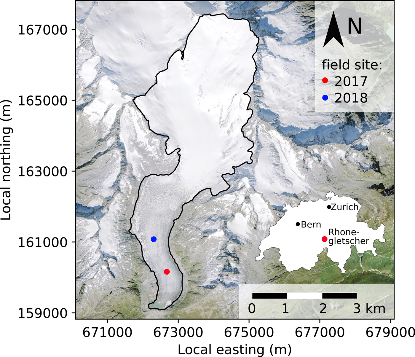
Fig. 1. Map of Rhonegletscher and its location within Switzerland (white polygon). The red dot indicates the field site in 2017, the blue one in 2018. Coordinates in LV03. (Ortho-image provided by Swisstopo and glacier outline in 2007 (Bauder and others, Reference Bauder, Funk and Huss2007))
The study site in 2017 (red dot in Fig. 1) is located at the lowest 10% of the tongue at ~2300 m altitude close to the flow line at LV03: 672750, 159950. A piezoresistive pressure sensor with a sampling frequency of 1 kHz was installed ~10 cm above the glacier bed in a (117 ± 1) m deep borehole, drilled with the hot water technique (Iken and others, Reference Iken, Röthlisberger and Hutter1976). The total time over which the pressure sensor recorded at the bed of the glacier is 51 hours excluding multiple recording interruptions. Further specifications of the instrumentation and experiment setup as well as times of data acquisition can be found in the Supplementary material.
HYDRAULIC OSCILLATIONS AT THE GLACIER BED
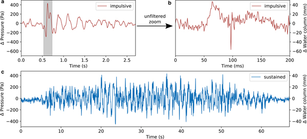
We visually scanned the recorded pressure time series and found different types of transient signals. Here, we note four types of events: The first two are non-resonant ones and include repeatedly occurring swarms of high frequency (250 Hz) pressure pulses, as well as slow pressure drops lasting longer than a second. The other two end-members are resonance phenomena. Among them, we find short resonances decaying within a few seconds (see Fig. 2a). These signals show a dominant frequency of ~4 Hz and we call them ‘impulsive’ events. Moreover, the record contains resonant signals lasting roughly one minute long (see Fig. 2c) with a dominant frequency of ~1 Hz, which we call ‘sustained’ events. While all sustained events show a rather gradual emergence and decay, impulsive events often show a gradual decay but an impulsive high-amplitude onset.

Fig. 2. (a) Waveform of an impulsive resonance event low pass filtered at 10 Hz. (b) Unfiltered zoom into the gray marked area of subplot (a). A non-dispersive sound wave becomes visible at ~ 90 ms. (c) Waveform of a sustained resonance event low pass filtered at 10 Hz.
We found clear signals from five sustained and 20 impulsive events in the 51 hour long record. Both types occur only during times of overall rising water pressure, similar to what Kavanaugh (Reference Kavanaugh2009) observed for strong pressure pulses on Trapridge Glacier, Yukon, Canada. The amplitudes of our measured resonances vary between 200 and 1100 Pa. Individual events cluster temporarily.
Impulsive events are occasionally accompanied by very short pressure pulses, lasting only a few milli seconds. One of these is shown in Fig. 2b, which is an unfiltered zoom into the gray shaded area of Fig. 2a. A superposed high-frequency peak that arrives ~90 ms after the onset of the pressure oscillation can be seen. Plots showing the waveforms and the spectra of all recorded crack waves can be found in the Supplementary material.
The energy within the detected pressure oscillations is several orders of magnitude smaller than the energy in the fracture resonances in previous studies that were detected and recorded by their emitted seismic waves (Anandakrishnan and Alley, Reference Anandakrishnan and Alley1997; Winberry and others, Reference Winberry, Anandakrishnan and Alley2009; Métaxian and others, Reference Métaxian, Araujo, Mora and Lesage2003; Stuart and others, Reference Stuart, Murray, Brisbourne, Styles and Toon2005; West and others, Reference West, Larsen, Truffer, O'Neel and LeBlanc2010). Consequently, a simultaneously deployed dense seismometer network at the glacier surface with a distance between stations of ~ 100 m and one seismometer placed ~ 120 m directly above the pressure sensor showed no seismic signature of the fracture resonances observed on the pressure sensor at the bed. From this we conclude that our recorded pressure oscillations are of much smaller magnitude than those detected in the previously mentioned studies, which show clear seismic signals.
CHARACTERISTICS OF CRACK WAVES
We interpret our resonant pressure oscillations as crack waves within the basal water layer sandwiched between the ice of the glacier from the top and the hard granite bedrock from below. Imagery from a co-located borehole camera supports this interpretation. The geometry of the basal conditions at the borehole terminus is schematically shown in Fig. 3a. The borehole with the pressure sensor connects directly to the water layer. The ice and rock react elastically to pressure oscillations within the water layer. Figure 3b shows an image from a borehole camera at the location where the resonances were recorded. It is a top view onto the hard bedrock showing pebbles on the granite bed and clast protrusions behind the almost transparent ice of the borehole margins. The borehole image confirms the possibility that the ice at the bedrock may be supported by clasts (Creyts and Schoof, Reference Creyts and Schoof2009). Furthermore it minimizes the possibility that the recorded crack wave resonances are accommodated within a channel or cavity since no three-dimensional (3-D) water-filled volume was present at the borehole terminus.
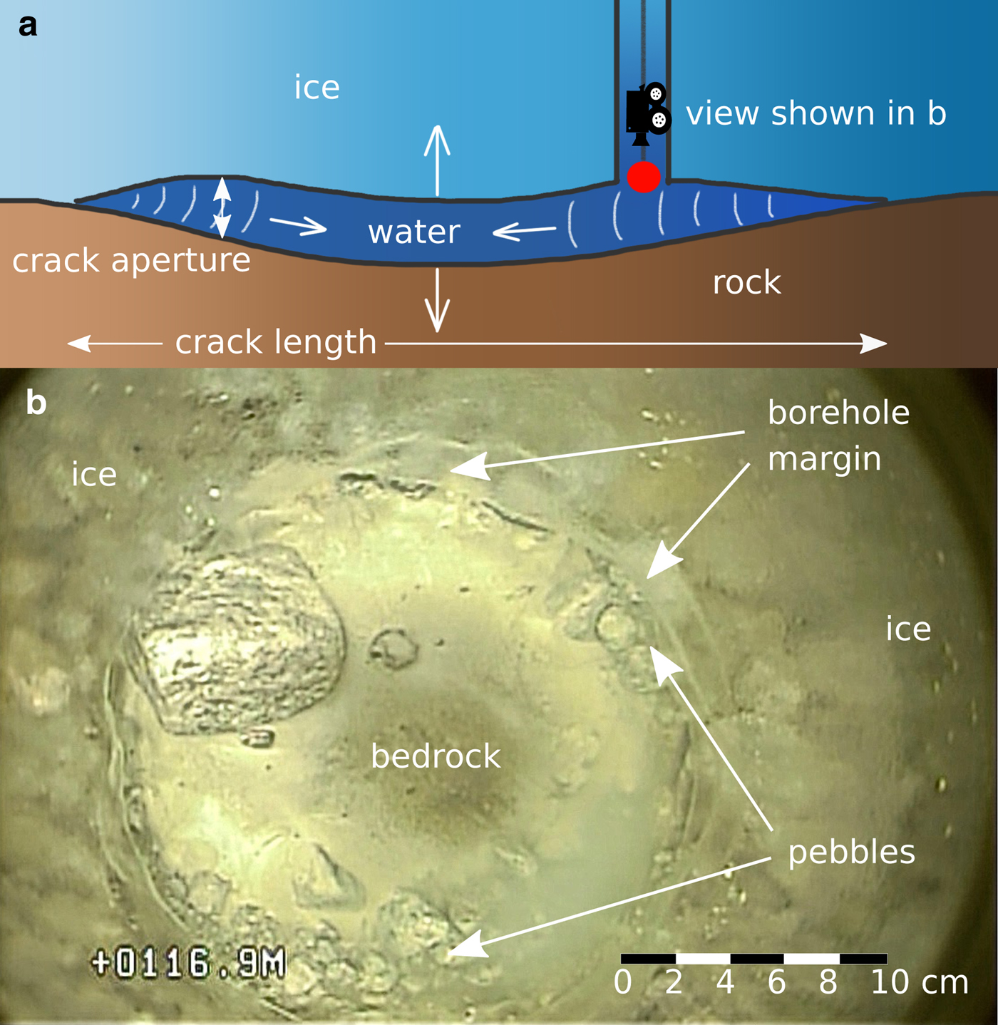
Fig. 3. (a) Scheme of crack waves within the basal water layer, a borehole camera and the pressure sensor (red dot), (b) top view from a borehole camera on the granite bedrock at the location of the pressure sensor.
The thin water layer at the ice/bedrock interface is geometrically similar to a water-filled fracture, and thus low-frequency resonances are expected to occur as pairs of counter-propagating crack waves along the finite extent of the water layer. Because the range of possible resonance wavelengths is constrained to be a multiple of the fracture length, crack waves propagating within the basal water layer show narrow-banded peaks in the frequency spectrum (Lipovsky and Dunham, Reference Lipovsky and Dunham2015, Eqn(91)).
Figure 4 shows the spectra of an example from the impulsive (red) and sustained (blue) crack waves. The gray dashed line shows the pre-event noise. The red and blue shaded areas indicate the one sigma error region of the mean spectra which represents the spectral content of the resonances best and shows the spectral peaks clearest. Both event types show distinct frequency peaks. Most prominent are the spectral peaks at ~1, 2 and 4 Hz that are visible in both the impulsive and sustained events. However, the relative power in these peaks differs between impulsive and sustained events. Whereas the spectral energy within these three peaks increases with higher frequency for impulsive crack waves, leading to a dominant frequency of ~ 4 Hz, sustained crack waves have their dominant frequency at ~1 Hz with a decreasing trend in the spectral power to higher frequencies. In addition, there exist two further peaks for the sustained events at ~6 and 8 Hz whereas the impulsive events have a broad, smeared-out peak at ~12 Hz. Gray shaded regions denote the width of the five lower frequency peaks at  $1/\sqrt {2}$ of the peak amplitude calculated from the full ensemble of events as described below (see also Supplementary material).
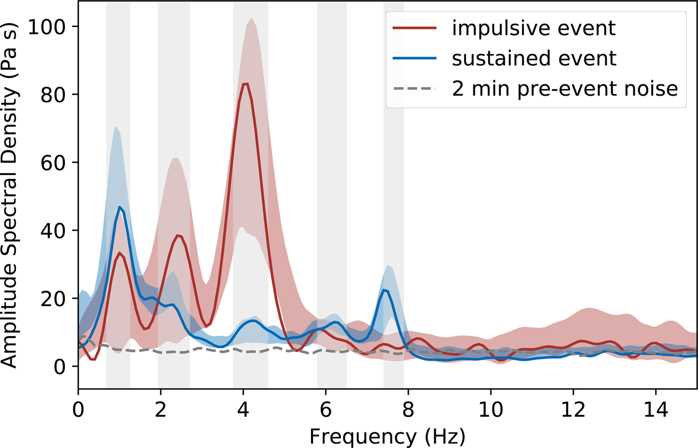
Fig. 4. Amplitude spectral density (ASD) of an example impulsive (red) and a sustained (blue) crack wave. The gray dashed line shows the pre-event noise level. Red and blue shaded areas indicate the one sigma uncertainty of the median ASD. Gray shaded regions mark the peak widths derived from a kernel density estimation (see Supplementary material).
The clear peak in the spectrum of sustained events at ~8 Hz that is not clearly visible in the impulsive events might be a hint that different modes are excited for different event types. This may be a source effect or a superposition of crack waves within different fractures or from different directions of the resonator volume. However, the similarity of the resonance frequencies occurring in the impulsive, as well as in the sustained crack wave resonances, is a strong indicator for a common resonance effect.
Borehole resonances
The borehole itself is an artificial water cavity that is capable of hosting resonances. To show that the resonances we measure are indeed crack waves traveling within the thin basal water layer and thereby justifying the use of the crack wave model of Lipovsky and Dunham (Reference Lipovsky and Dunham2015), we show in the following that we expect different frequency contents from pressure oscillations within the borehole.
Large pressure drops in the sub- and englacial water system are capable to excite resonances of the entire water column in the borehole. We expect these resonances to have a normal mode close to a harmonic oscillator of an open tube in a water reservoir with an angular frequency  $\omega = \sqrt {g\,h^{-1}}$, where g is the Earth's gravitational acceleration and h is the height of the water column (for a derivation see Eqns (A 4a) to (A 4b)). Assuming a water level of 100 m, which is similar to the water column we measure in the borehole, we expect a resonance frequency of order 0.1 Hz or less.
Resonances in water-filled fractures within the ice or at the bed can lead to so-called ‘tube waves’ within an intersecting borehole (Liang and others, Reference Liang, O'Reilly, Dunham and Moos2017). These travel within the borehole and interact with the elastic margins of it. For the tube waves, we expect resonance frequencies following the modes similar to an organ pipe f n = 4n c t h −1 with n = 1, 2, 3, … and the tube wave velocity c t (Eqns (1) & (2) in Roeoesli and others, Reference Roeoesli, Walter, Ampuero and Kissling2016; Biot, Reference Biot1952). By using a tube wave velocity of c t = 1100 ms−1, determined by Eqn (A 3), this leads to a fundamental frequency of f 1 = 2.75 Hz again with a water column of 100 m. Although some of the overtones we measured are of the same order of magnitude, the measured low fundamental frequency in the pressure oscillations cannot be explained by water column resonances and tube waves for our case. Moreover, we expect a wave that is strong enough to excite a resonance in the borehole by traveling up and down the entire borehole water column multiple times to be detectable with our surface seismometer array similar to what has been observed for seismic moulin tremor by Roeoesli and others (Reference Roeoesli2014, Reference Roeoesli, Walter, Ampuero and Kissling2016).
Dispersion of crack waves
Due to the interaction with the elastic walls, crack waves are dispersive and thus the overtones of the resonance are non-integer multiples of each other, enabling us to test if the resonances we measure are indeed crack waves. For closed fractures, possible resonant wavelengths are λn = 2 L n −1 with n = 1, 2, 3, … and the crack length L, and resonant frequencies  $f_n = c(\lambda _n)\,\lambda _n^{-1}$ (Lipovsky and Dunham, Reference Lipovsky and Dunham2015). This leads to an increasing spacing between the frequency peaks f n/f 1 = n 3/2 for crack waves. Our pressure oscillations do not perfectly follow the theoretical exponent of 3/2. From an ensemble analysis (see Supplementary material) of single crack wave events, we determine the fundamental frequency to f 1 = 0.98 Hz with a standard deviation of σf1 = 0.05 Hz and for the overtones f 2 = 2.30 Hz, σf2 = 0.11 Hz, f 3 = 4.18 Hz, σf3 = 0.08 Hz, f 4 = 6.14 Hz, σf4 = 0.19 Hz, f 5 = 7.61 Hz, σf5 = 0.19 Hz. This leads to an exponent in the dispersion relation of n ≈ 1.3 compared to 1.5 in the model of Lipovsky and Dunham (Reference Lipovsky and Dunham2015). However, it has to be emphasized that the equations represent an idealized setup by assuming a spatially uniform aperture of the crack and a surrounding homogeneous material (for further discussions of this topic, see Lipovsky and Dunham (Reference Lipovsky and Dunham2015)). We apply this model to a setup at a bi-material interface where the fracture is supported by protrusions, whereas Lipovsky and Dunham (Reference Lipovsky and Dunham2015) assumed that the aperture was supported entirely by a water pressure in excess of the overburden pressure. In any case, since our overtones in the spectrum do not represent integer multiples of the fundamental frequency, the measured resonances show a dispersive behavior. Thus we conclude that they plausibly represent crack waves within the thin basal water layer between the ice and the bedrock.
WATER LAYER PATCH SIZE
We use the crack wave resonances to estimate the extension of the resonant basal water layer patch using Eqns (A1) and (A2). The resonator length is determined to be L=19.8 m with a standard deviation of the single measurements of σL = 1.8 m and a systematic uncertainty of ΔL sys = 6 m due to the bi-material interface (systematics are described later in this section). The aperture is calculated to w=1.1 mm with σw = 0.3 mm. We give the standard deviation of the single value here, because the crack aperture, and probably also the crack length, vary with different water pressures as described in the section ‘TRANSIENT PRESSURE CHANGES’. In the following, we outline the calculation of the aforementioned dimensions.
The elastic material properties and the geometry of the resonance volume govern the normal modes that can be excited within it. Since the material properties of ice, granite and water are known, we can estimate the water layer volume from the measured crack waves. In order to do so, the frequency content of the resonances and the spectral peak width, reflecting the resonance attenuation, has to be analyzed (Compare to Eqns (1) and (2) as well as Eqns (A1) and (A2)).
We carry out peak detection for each crack wave spectrum followed by a fit of a Gaussian for each peak to determine the peak position f n together with its width Δf n defined as the full width at half maximum of the energy spectrum (units of Pa2). Due to changing hydrostatic pressures during the observation times of the crack waves, the resonance frequencies and peak widths of individual events may change over time. A kernel density estimation (KDE) with a width of 0.3 Hz is applied to the collection of all detected peak positions. Subsequently, another Gaussian fit is applied to the peaks in the KDE. From the width of these Gaussians, frequency ranges for the overtones of interest are determined. As the last step, all the Gaussians fitted to the peaks in the spectrograms of individual crack waves that lie within the determined frequency intervals from the KDE are taken to calculate a mean of the peak frequencies, a mean of the peak widths, and their standard deviations. The detailed analysis is described in the Supplementary material.
There is an ambiguity in distinguishing the fundamental mode f 1, which is important for an estimation of the fracture size, because our measurements do not follow exactly the expected dispersion relation from the model of Lipovsky and Dunham (Reference Lipovsky and Dunham2015). Thus we cannot easily use the overtones of the crack waves for calculation of the resonance volume. We suggest that the spectral peak at ~1 Hz reflects the fundamental frequency. This might not be immediately clear from the spectra and the waveforms of the impulsive events (compare to Fig. 2b), where this frequency could also be associated with the signal envelope. However, the fact that the same frequency peak ~1 Hz occurs also for the sustained crack waves, supports the assumption that this peak is indeed the fundamental frequency. With the ensemble of crack waves that we analyzed, we determine the fundamental frequency is f 1 = 0.98 Hz with a standard deviation of the single peaks of σf1 = 0.05 Hz. The peak width is Δf 1 = 0.64 Hz with σΔf1 = 0.17 Hz, which leads to a quality factor  ${Q_{f1} =f_1 \Delta f_1^{-1} = 1.5}$ with $\sigma _{Q_{f1}} = 0.4$.
The model of Lipovsky and Dunham (Reference Lipovsky and Dunham2015) describing crack wave propagation does not account for a resonator volume between half spaces with differing elastic properties. This setup is needed for a proper description of the crack waves within the basal water layer. In the model, the elastic plain strain modulus is only used for the calculation of the crack length, but not for the crack aperture, because the attenuation due to radiation of seismic energy at the walls is not included in the model we use, and is different from other models, which include seismic wave scattering (Frehner, Reference Frehner2013; Liang and others, Reference Liang, O'Reilly, Dunham and Moos2017; O'Reilly and others, Reference O'Reilly, Dunham and Nordstrm2017). As a result, we expect a factor of two in the crack length estimation for pure rock compared to pure ice (compare the elastic plain strain moduli in Eqn (A2)) This factor arises from the different shear moduli and Poisson's ratios of ice and the granite bedrock (see Appendix B). For the quantitative size estimation of the basal water layer patch, we take the mean of the resonator volume estimation for pure ice and pure granite and report the difference to each end-member case as a systematic uncertainty ΔL sys.
In three dimensions, the crack length from the 2-D model of Lipovsky and Dunham (Reference Lipovsky and Dunham2015) corresponds to the maximum 2-D extension of the resonator. Equations (A1) and (A2) together with the physical parameters of ice, rock and water (see Appendix B) lead to a length estimation of the basal water layer patch of L=19.8 m with a standard deviation of the single measurements of σL = 1.8 m and a systematic uncertainty of ΔL sys = 6 m. The aperture (thickness) of the basal water layer at our drilling site is determined independent of the elastic properties of the fracture walls to w = 1.1 mm with σw = 0.3 mm. A table of the extension of the water layer patch calculated from the overtones can be found in the Supplementary material.
TRANSIENT PRESSURE CHANGES
We infer an increasing water layer aperture that occurs coincident with a simultaneous rise in hydrostatic pressure. The estimated change in aperture is between 2 and 40% within 20 minutes. These coincident phenomena are consistent with an expected increase in basal water layer thickness due to elevated buoyancy forces. In the following we describe our quantitative estimation of the increasing aperture:
Figure 5 shows the transient evolution of the hydrostatic pressure at the glacier bed from 101.5 m water column to 102.1 m water column over a period of 20 minutes starting at 22 August 2017, 10:08 am. At our site, the 117 m ice reaches flotation level at a water column of 107 m. During these 20 minutes, five sustained and four impulsive crack waves occur. Immediately before the second impulsive crack wave, a pressure drop of ~500 Pa (5 cm water column) appears.
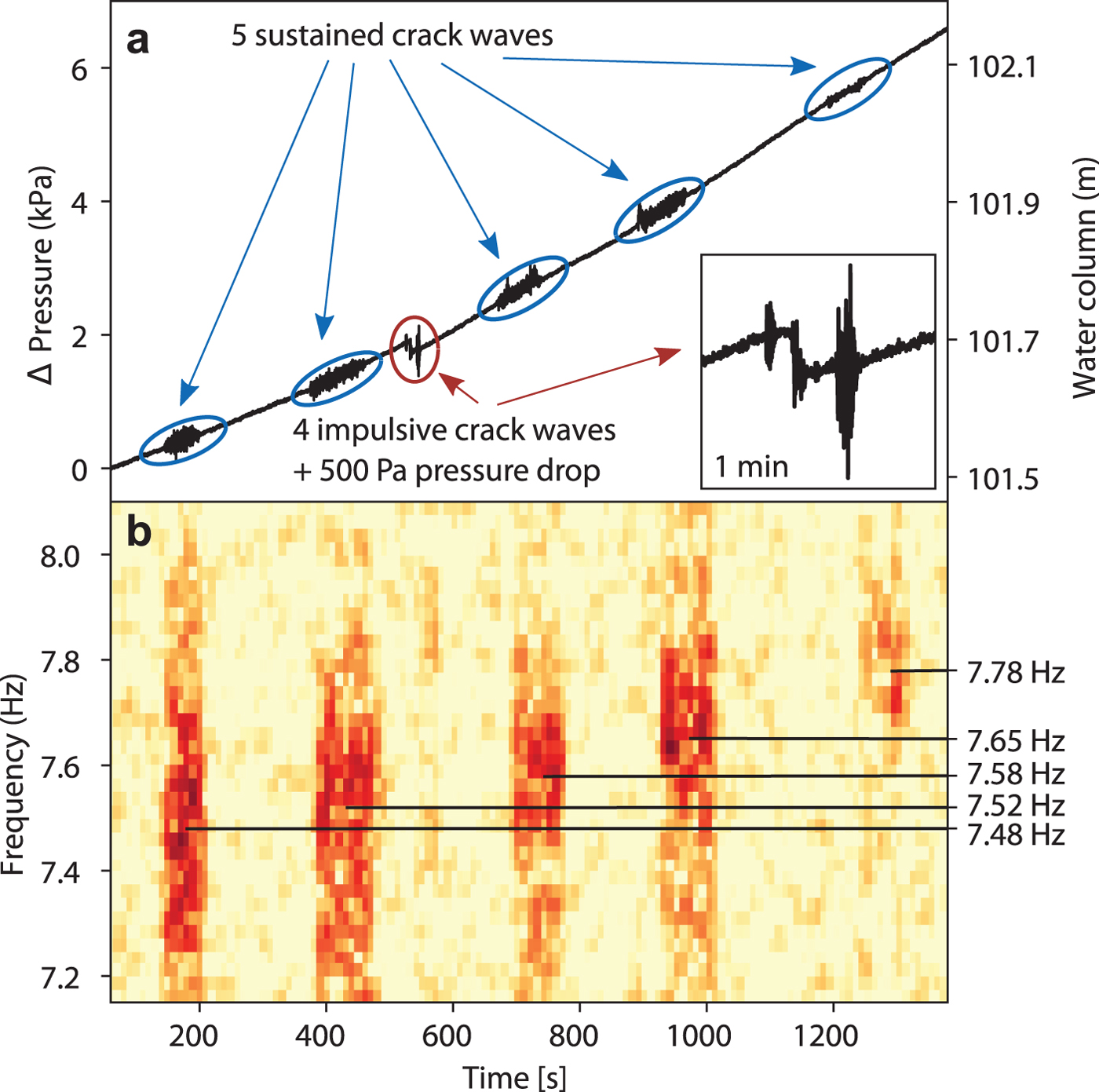
Fig. 5. (a) Temporal evolution of the relative pressure during the occurrence of five sustained crack waves within 20 minutes. (b) Spectrogram of one overtone between 7.2 and 8 Hz.
In the spectra of the sustained events, shown in Fig. 5b, an increase in the frequency content of the overtone below 8 Hz can be seen. A similar behavior has been observed by Heeszel and others (Reference Heeszel, Walter and Kilb2014) where resonance frequencies from hydro-fractures, recorded with surface seismometers, also increased over time. The authors explain this increase by a closing of the crack, which contrasts with our interpretation. This inconsistency may arise from the fact that Heeszel and others (Reference Heeszel, Walter and Kilb2014) did not take the attenuation of the signal into account, which plays a critical role for crack waves.
From the relative changes in the frequency content of the sustained crack waves in Fig. 5b it is clear that the geometry of the resonating volume must change. Eqns (1) and (2), which are also valid for overtones with f n and Δf n, predict that not only the frequency of the resonant peaks, but also their widths are affected by a changing crack geometry. While in the spectrogram in Fig. 5b a shift of the spectral peak of the overtone in the frequency band between 7.5 and 8 Hz from lower to higher frequencies can be seen, it is difficult to make statements about the peak width due to the limited frequency resolution in the spectra. From the peak analysis, a continuous increase in the peak frequency from 7.48 to 7.78 Hz can be determined. However, the peak width varies between 0.22 and 0.30 Hz with a decreasing trend. Assuming that there is no change in the width of the overtone, we estimate a minimal change in basal water layer aperture of Δw = 2% within 20 minutes. With this assumption, the length of the water layer patch would shrink by the same amount since both scale with the square root of the frequency. Including the trend in the spectral width of the overtone, the changes would be one order of magnitude larger with Δw = 40% and ΔL = 9%.
RESONANCE EXCITATION AND PRESSURE DROP
There are various candidates for resonance-exciting processes ranging from sudden basal cavity growth in response to stick-slip events (Zoet and others, Reference Zoet, Alley, Anandakrishnan and Christianson2013) or tensile faulting, (Walter and others, Reference Walter, Dalban Canassy, Husen and Clinton2013) to abrupt changes in fluid motion (Ferrick and others, Reference Ferrick, Qamar and St Lawrence1982; Julian, Reference Julian1994, although note countervailing analysis by Dunham and Ogden, Reference Dunham and Ogden2012). Since our study focuses on observed resonances rather than the processes which excite them, we only briefly touch on some of these aspects. Pin-pointing the exact excitation processes requires additional analysis and data, and is subject of ongoing investigation.
The high-frequency pressure pulse shown in Fig. 2c occasionally accompanies impulsive crack wave events, and may give further information on the triggering mechanism. Although we have not investigated this systematically yet, we suggest it is a non-dispersive sound wave traveling within the resonance volume of the basal water layer. However, we do not have an explanation for the delayed occurrence of the sound waves with respect to the onset of the crack wave resonances. The impulsivity of the sound waves in the pressure recordings hints towards an abrupt excitation mechanism such as a microseismic basal stick-slip event.
Crack waves that accompany rapid (~ms) pressure drops support the theory that basal microseismic stick-slip motion may be a possible trigger mechanism of impulsive crack waves. In Fig. 5a, a small pressure drop of ~500 Pa (5 cm water column) between the impulsive crack waves can be seen, while the overall hydrostatic pressure continuously increases. A similar event with a 2300 Pa (23 cm water column) pressure drop occurs 4 hours later (pressure curve in Supplementary material). In both cases, impulsive crack waves and other pressure oscillations similar to crack waves occur concurrently. The volume change producing a water column drop of 5 and 23 cm respectively, can be estimated from the geometry of the borehole, which has a diameter of ~15--20 cm. Assuming a weakly connected system, the opened volume is ~0.9--1.6 liter for the smaller pressure drop event and 4--7 liter for the larger one.
The simultaneous occurrence of impulsive crack waves in both cases together with the basal water pressure drop may be evidence for a microseismic stick-slip episode of glacier sliding (Zoet and others, Reference Zoet, Alley, Anandakrishnan and Christianson2013; Meierbachtol and others, Reference Meierbachtol, Harper and Humphrey2018): As a result of increasing water pressure caused by the diurnal melt cycle, decreasing effective pressure at the ice/bedrock interface decreases basal friction on sticky-spots (Fischer and Clarke, Reference Fischer and Clarke1997) near our pressure sensor. This means that shear stress accumulated at the ice/bedrock interface can exceed the decreasing frictional resistance, leading to stick-slip sliding triggering impulsive crack waves. A sudden volume change resulting from volume increase of water-filled cavities behind undulations in the bedrock during these stick-slip events causes the subglacial pressure drop.
Due to the temporal swarming behavior of the measured crack waves and the few events we have in our data, it is not possible to confirm with our crack wave data the prediction of Lipovsky and Dunham (Reference Lipovsky and Dunham2017) that the increasing hydrostatic pressure results in a shorter recurrence time of stick-slip events leading to a higher seismicity. This could have provided evidence for a relation between the crack waves and basal stick-slip events. However, the observation that crack waves in our data only occur with rising water pressure may indicate a link between increasing water pressure and basal seismicity from microseismic stick-slip events.
On recordings of a seismometer array (A field area map is in the Supplementary material.) that was deployed during our in-situ basal water pressure measurements, we could not find a signal of a basal stick-slip event during the pressure drops. One possible explanation could be that the stick-slip events causing the pressure drop and the crack waves were too small to be detected at the glacier surface.
SUMMARY AND OUTLOOK
The interpretation of the pressure signals as crack waves within the basal water layer was based on the following observations: The sustained and the impulsive pressure oscillations were recorded directly at the hard granite bedrock. Both show resonant behavior and they furthermore share common resonance frequencies, indicating a common resonance effect (i.e. crack waves). Non-equally spaced overtones support the interpretation of the pressure resonances as crack waves. Applying the formalism of Lipovsky and Dunham (Reference Lipovsky and Dunham2015) yields a reasonable thickness for the basal water layer, increasing with higher basal water pressures as expected for basal water pressure approaching flotation level. Further detected signals such as nearly instantaneous pressure drops and sound waves give hints towards a stick-slip related trigger mechanism.
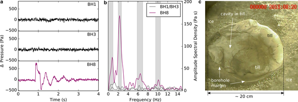
In 2018, we carried out similar measurements to 2017 but further up-glacier and with multiple pressure sensors. From these, we see indications that crack waves at the bed are not a unique phenomenon of the 2017 drilling site, but may be universal. Among many transient pressure pulses, drops and oscillations in the continuous 18-day-long data from 2018, we also found crack-wave-like events that are comparable to those measured lower on the tongue in 2017. (A field area map of the 2018 boreholes is in the Supplementary material. The position of the field site can be seen in Fig. 1)
Figures 6a and b show one of these potential crack wave signals from the 2018 dataset. As we had two additional simultaneously recording pressure sensors deployed that do not show any signal within a distance of 2.5 and 5 m from the sensor that recorded a signal, we suggest that the recorded resonance is a highly localized phenomenon at the glacier bed. Figure 6c shows borehole camera footage of the glacier bed in the direct vicinity of the crack wave resonator. Different from Fig. 3, a ~10 cm silt layer that can change within timescales of hours (see video in the Supplementary material) and that has the ability to tightly close water-filled volumes thus separating the resonator from the boreholes 1 and 3, may explain this observation. However, from the recorded resonance showing a dispersive frequency ratio of n 1.3 − n 1.5 similar to the 2017 crack waves, we can estimate a resonance volume length of L ≈ 12 m and a water layer thickness of w ≈ 1.7 mm which is comparable to the dimensions of the water layer patch measured lower on the glacier tongue. These measurements propose that using pressure resonances at the glacier bed is a promising method to study spatial and temporal variations of the basal water layer.
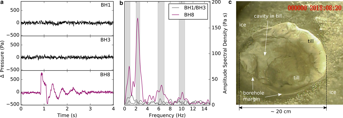
Fig. 6. (a) Waveform of a crack wave recorded at one borehole pressure sensor (BH 8). (b) Spectrum of the crack wave. (c) Footage of a neighboring borehole showing an at least 10 cm thick silt layer.
Although our results represent only point measurements, the length scales of the estimated water layer patches fit well to undulations in the bedrock that can be observed at the recently de-glaciated area of Rhonegletscher (see Supplementary material). Accordingly, basal water layer patches may form between bedrock bumps on which the weight of the overlying ice concentrates.
The thickness of the basal water layer of 1–2 mm that we determined is larger than previously estimated using sediment distributions to ~100 μm by Hallet (Reference Hallet1979). However, Hallet acknowledges that locally the thickness can be higher by a factor of 100. lndirect measurements of the water layer above an artificial till cavity at the subglacial laboratory at Engabreen show a thickness of up to 0.25 mm (Iverson and others, Reference Iverson2007). On the theoretical side, Walder (Reference Walder1982) calculates that the water layer thickness must be <5 mm for glaciers <100 km long, whereas Weertman (Reference Weertman1972) calculates millimeter-thick water layers for glaciers in the same size class as Rhonegletscher. Our in-situ measurements of the water layer thickness at our drilling site match these predictions well and represent a new method to investigate the extension and morphology of the basal water layer.
CONCLUSION
Kilohertz-sampled pressure measurements in the direct vicinity of the glacier bed of Rhonegletscher show resonant pressure oscillations with non-equally spaced overtones. We interpret these resonances as crack wave resonances within the basal water layer. A systematic relation between the resonant frequencies of these crack waves, their spectral width and a transient subglacial water pressure evolution was found. From these crack waves, the local thickness of the basal water layer and the extension of water layer patches that host the observed crack waves were determined. The results show that the basal water layer is sufficiently patchy to host crack wave resonances, and that it is a dynamic system, influenced by hydrostatic pressure changes.
DATA AVAILABILITY
In the future, the presented dataset will be made publicly available on the servers of the Swiss Seismological Service (http://seismo.ethz.ch). The network name is ‘4D’ and the station name is ‘RA01P’. In the meantime the dataset is available on request from the author. The python code for the data analysis is included in the Supplementary material.
SUPPLEMENTARY MATERIAL
The supplementary material for this article can be found at https://doi.org/10.1017/aog.2019.8
ACKNOWLEDGMENTS
We thank the two anonymous reviewers for their constructive comments on this paper and our colleagues at VAW for their great support in the field. Financial support was provided by the Swiss Federal Institute of Technology (ETH Zurich) via Grant ETH-06 16-12 and the ETH Scientific Equipment Program as well as the Swiss National Science Foundation (Grant PP00P2_157551).
APPENDIX A. EQUATIONS
Fracture length from Lipovsky and Dunham (Reference Lipovsky and Dunham2015) in the crack wave limit with the kinematic viscosity of water ν, the density of water ρ0, the elastic plain strain modulus G*, the fundamental frequency of the resonance f 1, and its attenuation factor Q 1:
 $$ L = {1 \over 2} \left[\pi\,\nu \left({G* \over \rho_0}\right)^2 {Q_1^2 \over f_1^5}\right]^{1/6} $$
Full fracture aperture from Lipovsky and Dunham (Reference Lipovsky and Dunham2015) in the crack wave limit with the kinematic viscosity of water ν, the fundamental frequency f 1 and its attenuation factor Q 1:
 $$ w = Q_1 \ \sqrt{{\nu \over \pi\,f_1}} $$
Tube wave velocity from Roeoesli and others (Reference Roeoesli, Walter, Ampuero and Kissling2016) with the bulk modulus of water b, the shear modulus of ice G and the density of water ρ0:
 $$ c_t = \sqrt{{G\,b \over \rho_0\,(G + b)}} $$
Gravitational oscillations (angular frequency ω) of a water column (mass m tot, density ρ) with height h in a tube with diameter r, the earth acceleration g, and the water level deviation from the equilibrium position y(t):
 $$F(t) = m_{tot} \, \ddot y(t) = \rho \pi r^2\,h \, \ddot y(t) \, {\rm and}$$
 $$F(t) = - \rho \pi r^2 y(t) \, g $$
 $$ \rho \pi r^2\,h \ddot y(t) = - \rho \pi r^2\,g \ y(t) \hskip 8pt{\vskip -7pt\mathop{\rm oscillatory} \limits_{\overrightarrow{\rm solution}}} \quad \omega = \sqrt{{g \over h}} $$
APPENDIX B. PHYSICAL PARAMETERS
List of physical parameters used for crack geometry determination and tube wave velocity (Lipovsky and Dunham, Reference Lipovsky and Dunham2015; Petrenko and Whitworth, Reference Petrenko and Whitworth1999):
Shear modulus: G = 3.8 GPa for ice, G = 27 Pa
Bulk modulus of water b = 1.98 GPa
Kinematic viscosity of water: ν = 1.7 · 10 −6 m2s−1
Poisson's ratio: ν s = 0.35 for ice, ν s = 0.25 for granite
Density of water: ρ0 = 1000 kg m−3


 Open access