Introduction
Berkner Island holds a marine ice sheet which is independent of the Antarctic ice sheet at present (Fig. 1). Surrounded by the Ronne and Filchner Ice Shelves, it rises to a northern (720ma.s.l.) and a southern dome (890ma.s.l.) 50 and 200 km from the open sea in summer, respectively. Meteorological (Reference Reijmer, Greuell and OerlemansReijmer and others, 1999) and field observations show that the domes are not affected by the katabatic wind regime; and due to the dome topography they are expected to provide a good climatic record of the Weddell Sea region.
Fig. 1. Map of Berkner Island and the Filchner–Ronne Ice Shelf area. The drill sites of cores R1 (Reinwarthohe, north dome) and B25 (Tyssenhohe, south dome) are indicated. Also shown are two sites on the Antarctic Peninsula discussed in the text.
In 1989/90 two 11 m deep firn cores were recovered from the domes, which showed clear seasonal cycles and a marked concentration decrease of marine tracers with increasing distance from the coast (Reference WagenbachWagenbach and others, 1994). Two cores of intermediate depth were drilled during the 1994/95 joint field seasons of the Alfred Wegener Institute (AWI), Germany, and the British Antarctic Survey. The cores reached depths of 151 m (R1, north dome) and 181 m (B25, 5 km from south dome) and span approximately 600 and 1200 years, respectively. Currently, a deep drilling at the south dome is underway as a European Programme for Ice Coring in Antarctica (EPICA) associated project; a core to bedrock is expected to include the ultimate deglaciation if Berkner Island was not overrun by the Antarctic ice sheet.
First results from the intermediate cores have been published, focusing on R1 (Reference MulvaneyMulvaney and others, 2002). Here we present a revised dating of the B25 core; chemical and isotopic time series for both cores are shown and discussed.
For the chemical analyses of the B25 core a set-up for continuous ice-core melting was used that also provided samples for subsequent standard ion chromatography (IC) measurements. This new development is also presented here.
Ice-Core Analysis
The B25 ice core was analyzed continuously using a combination of discrete sampling and continuous flow analysis (CFA) methods. Electrical conductivity measurements (ECM) on the frozen ice core were performed in the field, and density was measured at high depth resolution in the cold laboratory at AWI in Bremerhaven (Reference Gerland, Oerter, Kipfstuhl, Wilhelms, Miller and MinersGerland and others, 1999). Samples for δ18O and δD were cut in roughly annual resolution. Electrolytical conductivity σ, Ca2+, NH4 + and water-insoluble microparticle concentrations were measured in a CFA system at an effective depth resolution better than 1.0 cm. F–, MSA–, Cl–, NO3 – and SO4 2– concentrations were measured by IC at sample resolutions of 2.0– 6.5 cm; these samples were not cut and decontaminated individually, but prepared using the CFA system, a novel method of sample preparation that is now being applied widely within the EPICA project. While the ECM and stable-isotope measurements are described elsewhere (Reference MulvaneyMulvaney and others, 2002), the chemical analyses are detailed below. Stable-isotope and ECM measurements were performed on the whole core; the chemical analyses were performed from the top to ≈150m depth.
The melting device
An apparatus for continuous ice-core melting has been developed at the Institute of Environmental Physics (IUP), Heidelberg, Germany, for operation in a warm laboratory. It consists of a freezing unit to prevent uncontrolled melting of the ice core, and a melt head (MH) which is mounted at the bottom of the unit, for controlled ice-core melting (see Fig. 2). The cylinder-shaped freezer hosts a concentric tube of Plexiglas to guide the core to the MH. The MH has two concentric sections that are drained separately, and only the sample from the inner, clean part of the ice core is used for the analyses, while the sample from the outer, possibly contaminated part is discarded. The MH is specially designed for processing porous firn cores. It is made from anodized aluminium and has narrow slits for this purpose (see Reference RöthlisbergerRöthlisberger and others, 2000b; Reference SommerSommer and others, 2000a, Reference Sommer, Wagenbach, Mulvaney and Fischerb). The whole unit is rotatable into horizontal position to load it with a new ice core or for service. Each melt run started with a 5 cm long strip of artificial Milli-Q ice to ensure stable melting conditions once the real sample reached the MH. The freezer may be evacuated and purged with N2 gas to reduce gaseous contaminations when melting firn. Typical melt-parameter values included a freezer temperature of –20˚C and a MH temperature of +20˚C; this resulted in typical melt speeds of 2.6 cm min–1 for ice and 3.9 cm min–1 for firn. The meltwater runs first through a debubbler and is then pumped by peristaltic pumps into individual flowlines for analyses.
Fig. 2. Schematic illustration of the measuring set-up including the melting apparatus (left) and the analytical flow system (right); the automatic sampler is enlarged. Numbers indicate typical flow rates in mL min–1.
The samples for discrete IC measurements were taken from the flowline of the electrolytical conductivity and particle measurements, neither of which contaminate the sample. The liquid was filled directly into pre-cleaned Dionex polyvials (5 mL) which could be transferred directly into a Dionex autosampler for subsequent IC measurements. To switch from one vial to the next, a modified Dionex autosampler was used controlled by an external computer. In order not to lose sample during vial exchange (≈25 s) a buffer reservoir was employed. With such a set-up, a depth resolution of better than 1.0 cm is possible for the IC samples depending on the MH dimensions, the number of ‘destructive’ CFA lines used and the amount of liquid needed for each sample. In the current applications within the EPICA project, Coulter Counter accuvettes are used in custom-built autosamplers.
Samples for IC were not measured right away because of organizational constraints. They were refrozen directly after preparation and kept frozen until measurement. The whole procedure was checked against contamination. Taking ultraclean Milli-Q water as sample, contamination was monitored at three stages of the processing: the IC measurement alone (‘IC blank’), the IC measurement including one freeze–thaw cycle (‘freeze blank’), and the whole preparation process including cutting and melting via the MH (‘process blank’). It was found that the extra freeze–thaw cycle for storage is not a source of contamination (see Table 1); however, sample preparation through melting leads to significant contamination in SO4 2–, exceeding 10 ng g–1.
Table 1. Blank concentrations of the IC samples in three different categories as described in the text. All values in ng g–1

The MH was found to be the source, but the contamination was not eliminated. It may stem from particulates that are stuck in the interior construction of the MH and could not be washed out even under ultrasonic exposure. Another possibility is that the anodized aluminium of the MH itself is responsible, as the anodizing takes place in concentrated sulphuric acid; this seems unlikely, though, since the contamination was zero at the beginning and was detected only after some usage. The contamination does not pose a severe problem in this application because non-sea-salt (nss) SO4 2– concentrations are normally of the order of 100 ng g–1 in Berkner Island samples, i.e. well above the level of contamination.
Detection systems and data analysis
The electrolytical conductivity measurement was done using an electronic detector by Dionex or WTW together with a Dionex or a self-built cell, respectively. Water-insoluble microparticles were measured with a laser counter developed by Klotz Company in collaboration with the IUP (see Reference Ruth, Wagenbach, Bigler, Steffensen, Röthlisberger and MillerRuth and others, 2002, Reference Ruth, Wagenbach, Steffensen and Bigler2003). The CFA systems for Ca2+ and NH4 + were provided by the University of Bern, Switzerland. The IC measurements used a Dionex DX 500 with an AS12 anion separator column.
Data analysis included in a first step the conversion of recorded detector outputs to calibrated concentrations. The time lags from sample melting until detection are different for each system and needed to be corrected individually to avert systematic errors in seasonal phasings.
The non-sea-salt contribution to conductivity σnss was calculated from the measured electrolytical conductivity σ by subtracting the sea-salt contribution as calculated from the Ca2+ concentrations: σnss = σ – k[Ca2+]; k was derived experimentally, and k =0.176 μS cm–1 (ng g–1)–1 was used. The calculation of nssSO4 2– concentrations was based on [Cl–]; it needs to account for aerosol fractionation, and the ion ratio from sea water does not apply; following the investigations by Reference Minikin, Wagenbach, Graf and KipfstuhlMinikin and other (1994), [SO4,nss2–] = [SO4 2–] – 0.0315[Cl–] was used.
Dating
Owing to the accumulation rate of 130 kgm –2 a–1 (see below) and the high-resolution measurements, seasonal cycles could be identified for several components throughout most of the core. Thus, dating was achieved by multiparameter counting of annual layers. However, the seasonal variations were ambiguous at times, as all components measured at sub-seasonal depth resolution may show multiple annual peaks. Therefore, to achieve a core chronology with long-term reliability it was necessary to constrain the dating by selected volcanic horizons.
Counting of seasonal cycles
As is explained below, the austral winter layer was marked for each year. Figures 3 and 4 give examples of seasonal variations with distinctness above and below average, respectively. Seasonal variations were most obvious in ECM and Ca2+ signals. The ECM signal represents mainly the concentration of free H+, which is higher in austral summer than in winter. This seasonal variation is amplified by events of high sea-salt input, which occur mainly during winter and cause a drop in the ECM signal to zero, thus forming a good indicator for austral mid-winter layers. However, occasional strong inputs of mineral dust aerosol, which may occur mostly during the summer months, or an unusual summer-time sea-salt event can also cause a reduction of the ECM to zero. Therefore, the ECM signal is not strictly seasonal, and layer counting based on ECM alone will be somewhat unreliable.

Fig. 3. Example of annual layers (distinctness better than average). Vertical lines mark austral mid-winter (July) layers as from the annual-layer counting.

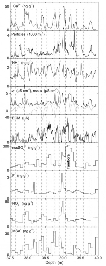
Fig. 4. Example of annual layers (upper panels; distinctness below average) and the Tambora volcanic horizon used for dating (lower panels). Vertical lines mark austral mid-winter layers. F– NO3 – and MSA– exhibit post-depositional redistribution around the Tambora layer.
At Berkner Island, Ca2+ is derived predominantly from sea-salt aerosol and to a lesser extent from mineral dust. At coastal Antarctic sites the sea-salt aerosol is deposited mainly during mid-winter (e.g. Reference WagenbachWagenbach and others, 1994, Reference Wagenbach1998); this was commonly believed to be due to the greater storm activity during that season, but now the seasonally greater extent of sea ice, which serves as an effective source for sea-salt aerosols through frozen brine and frost flowers, is shown to be the driving mechanism (Reference WagenbachWagenbach and others, 1998; Reference Rankin, Auld and WolffRankin and others, 2000). Usually, there are several Ca2+ peaks every year, but normally there is a dominant one. Therefore, large Ca2+ peaks were taken as markers for mid-winter horizons.
Berkner Island has no areas of exposed rock, and mineral dust particles must have been transported long distances. It is currently being investigated whether the dominant dust sources for Berkner Island are Patagonian or other South American deserts, as is believed for East Antarctica based on isotopical and mineralogical studies (Reference Basile, Grousset, Revel, Petit, Biscaye and BarkovBasile and others, 1997), or whether other sources are also important. At Berkner Island, dust concentrations usually peak several times a year and do not show a clear seasonality (see Fig. 3 and 4). This is similar to the observation by Thompson and others (1994) for ice cores from Dyer Plateau and Siple Station, both on the Antarctic Peninsula, and is contrary to results from a few aerosol measurements and high-resolution firn studies at Neumayer station (Reference Wagenbach, Wolff and BalesWagenbach, 1996) and South Pole (Reference Mosley-ThompsonMosley-Thompson, 1980; Reference Tuncel, Aras and ZollerTuncel and others, 1989), which indicate maximal crustal concentrations during mid-summer. At Berkner, dust peaks usually occur independently of sea-salt peaks, but sometimes they are concurrent. The high-resolution dust profiles played only a secondary role in the counting of annual layers; the presence of a strong dust peak prohibited the assignment of a winter layer based on an ECM minimum alone, and it raised questions about the assignment of a winter layer based on a sea-salt peak.
NH4 + also showed marked variations, but they appeared to be mostly sub-seasonal (see Fig. 3 and 4). In contrast to Ca2+, there was not normally one dominant peak every year. NH4 + peaks are sometimes associated with dust or with sea-salt events, but they may also occur fully independently. NH4 + seems to be derived from multiple sources (continental and possibly marine) or seems to follow multiple transport pathways. The NH4 + variations were irregular in strength and timing and therefore were not used as primary indicators for annual layers. But as the source strength for NH4 + may be expected to be seasonal and highest in summer (Reference Legrand, Ducroz, Wagenbach, Mulvaney and HallLegrand and others, 1998), we used peaks of NH4 + as soft contraindicators for winter layers in the counting procedure.
Another useful parameter for counting annual layers was the non-sea-salt conductivity σnss. While σ peaks in midwinter due to the high sea-salt concentrations, σnss is found to peak in mid-summer (see Fig. 3 and 4), which suggests acidic aerosols (mainly biogenic SO4 2– and HNO3). However, no priority was given to σnss since it is a derived measure, and small errors in the peak phasings or shapes of [Ca2+] and σ can lead to large artefacts in σnss.
It proved most practical to mark the mid-winter horizons in the core for each year, as the sea-salt events were the most regularly observed and most prominent events in the record. These horizons were taken as July of the respective year. Accordingly, the annual averages presented below were taken from July of the assigned to July of the previous year.
Volcanic markers
The layer counting was constrained by unambiguously identified volcanic horizons. Unfortunately, these horizons are few because volcanogenic SO4 2– often cannot be clearly identified. This is mainly due to the large quantities of sea-salt-derived SO4 2– and marine-biogenic SO4 2– which obscure the volcanogenic contribution; also, because of possibly volcanogenic Cl– contributions, the use of Cl– as a sea-salt indicator may weaken volcanic SO4 2– peaks.
Figure 4 shows the volcanic horizons of Tambora, Indonesia (eruption AD 1815), and Figure 5 the ‘1259– unknown’ sequence. These are the two volcanic events identified most clearly in the B25 core. Such identifications are based on (i) enhancement of ECM and/or ECM winter minimum not going completely to zero, (ii) enhancement of nssSO4 2–, (iii) NO3 – and MSA migrated outward (see below), and (iv) possibly F enhancement. A list of all identified volcanic events is given in Table 2.
Fig. 5. The volcanic sequence of 1259–unknown and thereafter. Vertical lines (full length) indicate the well-known quadruple of events (e.g. Reference Langway, Osada, Clausen, Hammer and ShojiLangway and others, 1995); numbers denote years (AD) according to the B25 chronology derived here. Half-length vertical lines indicate possible additional volcanic events previously unrecognized.
Table 2. List of all identified volcanic events in the B25 core decrease from north dome to south dome, as expected. It is noteworthy that nssSO4 2– concentrations are higher at south dome, while MSA concentrations are slightly lower. This is contrary to Reference WagenbachWagenbach and others (1994) who found nssSO4 2– lower at south dome by 25%; however, Reference Minikin, Wagenbach, Graf and KipfstuhlMinikin and others (1994) found very little dependence on the distance from the coast for nssSO4 2– concentrations in the Filchner–Ronne Ice Shelf area.
It should be noted that the nssSO4 2– peak of the Huaynaputina (Peru) horizon (AD 1600), which was rather minor, was not used alone to identify the volcano. Instead, the horizon was recognized based on a combination of a nssSO4 2– peak and a preceding particle peak, which is very distinct. Such a signature is reported by Thompson and others (1994) for the Dyer Plateau and Siple Station ice cores and dated from AD 1598 to 1600.
Results and accuracy
The resulting depth–age relationship, shown in Figure 6a along with the volcanic fix-points used to guide the layer counting, is a rather smooth curve. Also shown is the 1954 Tritium Horizon (Reference HukeHuke, 1998) from the neighboring B24 core (1m apart) which was used to confirm the dating. The preliminary dating by Reference MulvaneyMulvaney and others (2002) is revised by up to 15 years in the part above and by up to 40 years in the part below the 1259 volcanic horizon.
Fig. 6. (a) The core chronology obtained for the B25 ice core by annual-layer counting (solid line). Solid symbols mark the volcanic horizons used to constrain the layer counting; the open symbol marks the 1954 tritium horizon (Reference HukeHuke, 1998). The Nye model (see text) is indistinguishable from the solid line shown. (b) Age difference between the core chronology and the Nye model. (c) Frequency distribution of the annual net accumulation as derived from the core chronology (strain-corrected).
A simple ice-flow model was applied to fit the surface and the 1259 horizon (Reference NyeNye, 1963). For a proposed ice-sheet thickness of 850mw.e., which corresponds to approximately 950m of true ice thickness, parameter optimization yields an average accumulation rate of A = 130 kg m–2 a–1. The deviation of the counted core chronology from the Nye model is always <12 years and typically around 5 years (see Fig. 6b). The good agreement shows that, as a first-order approximation, the accumulation rate was fairly constant over the time covered, and that the simple ice-flow model may be applied to the 181 m long B25 core to obtain a first-order chronology.
The flow model was used to calculate a strain correction for each annual-layer thickness as derived from the counting. This yields the net accumulation for each year. The frequency distribution of the annual net accumulations is shown in Figure 6c in a histogram plot. It exhibits approximately log-normal behaviour, with a maximum around 130 kg m–2 a–1 and no sharp cut-off at either side.
The accuracy of the dating in between two volcanic fix-points was estimated experimentally by repeated counting of the same interval by six different persons. This yielded that for any point P which is n years apart from the nearest fix-point, the dating accuracy is better than ![]() . The same accuracy is inferred from the dating error when originally the layer counting had not been forced through the volcanic horizons. Ba
. The same accuracy is inferred from the dating error when originally the layer counting had not been forced through the volcanic horizons. Ba
Results
Average values of characteristic measures are given in Table 3 for both cores. Sea-salt components show a clear
Table 3. Characterization of the two drill sites and average values over the full core; for B25, averages are also given for the period covered by R1

Time series
The time series of selected components are presented in Figure 7. In general they show a 1000 year record of relatively stable climate and environmental conditions. Only small trends are observed for all measured components over the past 1000 years; the variability of the smoothed datasets is only moderate and takes place mainly on multi-decadal to centennial time-scales, while the variability of the annual averages may be substantial. Smoothing was done by 500 iterations binomial filtering of three points, which corresponds to a Gaussian average with full width at a 1/e maximum of 63 years or σ = 31.6 years. Figure 7 also shows data of the core R1 from the Berkner Island north dome. There is a large amount of variability between the two cores and only limited covariation. In the following, selected components will be discussed individually.
Fig. 7. Time series of the B25 core (solid lines, left scale) and of the R1 core (dotted lines, right scale). Fine lines are annual averages (B25 only); heavy lines are smoothed using a 500 iterations binomial filter (see text). Note different scales for the two cores in each panel: scales are set for both cores such that axes ranges divided by the respective data means are the same for both cores, i.e. relative variations are directly comparable by eye. Letters mark selected identified volcanic events: a. Agung; b. Krakatoa (uncertain); c. Tambora; d. Huaynaputina; e. Kuwae; f. 1259. The SO4 2– measurements suffered from system malfunction for AD 1200–1300, and calibrations may be uncertain there. Microparticle concentrations are for particles >1.0 μm in diameter.
The temperature proxy δ18O shows no first-order trends over the whole record, and a peak-to-peak amplitude of the multi-decadal variations in the order of 1%. The most prominent feature is a pronounced cooling during most of the 19th century by more than 1% in the smoothed data of B25. The record also shows an isotopically warm period from approximately AD 1230 to 1450, but no features may obviously be associated with the Little Ice Age (LIA) or the Medieval Warm Period (MWP) as they are known from some European or Greenlandic records (e.g. Reference FischerFischer and others, 1998). Also, the period of the Maunder Minimum of sunspot numbers (AD 1645–1715) is not unusual in the record. There is a recent warming trend, but it does not exceed by magnitude or rate earlier changes in the record. The records from Berkner north and south domes do not show a clear covariance on multi-decadal or centennial time-scales; this may reflect varying circulation patterns effective for the area. In both cores, the annual net accumulation shows a clear
enhancement during the period AD 1800–50. There is also an increase during the 20th century, as also seen throughout the Antarctic Peninsula and at South Pole (Thompson and others, 1994; Reference Mosley-ThompsonMosley-Thompson and others, 1995). No clear relationship is seen between δ18O and the annual accumulation, underlining the complicated meteorological situation of the Weddell Sea and Antarctic Peninsula region. Apart from the two covariant periods mentioned, the accumulation rates of the two cores exhibit a contra-variant behaviour. This could result from storms hitting either the north or the south dome more frequently. A remarkable feature is exhibited from AD 1475 to 1500: this period is characterized by a dramatic decrease in accumulation and a substantial cooling; there are low Cl– concentrations throughout the period until it terminates with one of the highest Cl– values in the record.
The sea-salt-derived component Cl– varies slightly and does not seem to depend on δ18O in either core. The two Cl– records are not closely related to each other, which again may be the result of variable regional circulation patterns. There are two periods of elevated sea-salt concentrations in B25: AD 1400–1570 and AD 1830–1900. These could be caused by increased storminess during that time or by increased or prolonged sea-ice extent. δ18O does not indicate a cooling during either of the periods; however, the relationship between δ18O at Berkner and sea-ice extent in the Weddell Sea is unknown. Reference Kreutz, Mayewski, Meeker, Twickler, Whitlow and PittalwalaKreutz and others (1997) observe a marked increase of sea-salt tracers in Siple Dome, Antarctica, at AD 1389±12, which they attribute to a postulated global event of enhanced atmospheric circulation connected with the LIA. The beginning of the corresponding increase may be recognized at AD 1405°6 in the B25 core. Although this might suggest increased atmospheric circulation at a few selected Antarctic sites, this is not seen throughout Antarctica. Reference Sommer, Wagenbach, Mulvaney and FischerSommer and others (2000b) report no change of sea-salt-derived Na+ concentrations at Dronning Maud Land for the time around AD 1400. There is no coverage from R1 for that time.
NssSO4 2– is dominated by marine biogenic contributions. Both cores show an enhancement in the time period AD 1750–1850. The variability is more pronounced in the R1 core, reflecting its proximity to the open ocean. A higher variability in R1 is also observed for MSA– (see Fig. 8). The variations in MSA– are in phase in both cores, although the MSA– record is disturbed in B25 (see below). Overall, MSA– is the component that shows the best correspondence in both cores.
Fig. 8. Loss of MSA presumably during sample storage for B25 (upper panel); loss and contamination of NO3 – (lower panel). Annual means (thin lines) and 500 iterations binomially smoothed values (heavy line) for B25; smoothed values are shown for R1. The vertical arrows mark 0.85 g cm–1 density for each core. See text for discussion.
The microparticle record shows some prominent peaks even in the annually averaged data. Contamination was ruled out for each peak individually, and the peaks seem real at least in the part older than AD 1800. Most of the outstanding peaks are suspected to be of local volcanic origin; mineralogical studies should be performed to check this hypothesis. The prolonged enhancement of particle concentrations from AD 1200 to 1350 may be due only in part to the volcanic activity during that time and may also be due to increased mineral dust source strength or transport efficiency. The large increase in particle concentrations in the more recent part of the record, however, may be due to contamination of the firn during drilling and handling of the core. Thompson and others (1994) also observed a strong, recent increase of particle concentrations on the Dyer Plateau, but their measurements may suffer from the same problems (Thompson and others, 1994). The enhanced particle concentrations from AD 1650 to 1710, i.e. during the Maunder Minimum of sun-spot numbers, may be significant; however, nothing equivalent is observed during the Spörer Minimum (AD 1420– 1500) or the Wolf Minimum (AD 1290–1340).
To investigate the mutual dependence of temperature (δ18O), accumulation, and sea-salt (Cl–) concentrations, correlation coefficients were calculated and a principal component analysis (PCA) was carried out for B25. The correlation coefficients are all negligible (δ18O–acc. = 0.07; O–Cl– = –0.16; acc–Cl– = –0.11), i.e. very little interdependence of the data. Similarly, the PCA finds three principal components with an explained total variance of 41%, 31% and 28%, i.e. there is almost no redundancy in the data. This indicates a complex meteorological situation and suggests very variable storm-track patterns in the area.
Post-depositional changes
Post-depositional redistribution is observed for MSA–, NO3 – and F– at volcanic horizons. In Figures 4 and 5 it can clearly be seen that layers with high nssSO4 2– concentrations contain no significant amounts of MSA–, NO3 – and F–. For MSA– a seasonal redistribution has already been observed in other cores (Reference WagenbachWagenbach and others, 1994), and laboratory experiments have been performed to investigate the process (Reference Pasteur and MulvaneyPasteur and Mulvaney, 2000); Reference Weller, Traufetter, Fischer, Oerter, Peel and MillerWeller and others (2004) observe a net loss of MSA– in snow pits and shallow cores from Dronning Maud Land, which they explain by transport of MSA in the vapour phase. In B25, we see that MSA– tends to migrate away from the acidic layer and accumulate above the volcanic horizon. Presumably, the mechanism for the displacement is vapour-phase diffusion in the firn air. The large amount of H+ from the volcanic H2SO4 causes the concentration of gaseous MSA in the firn air to be locally elevated, which leads to a net transport of MSA away from the volcanic layer. Why the MSA accumulates above and not below the acidic layer remains unexplained.
The same is observed for NO3 –, which is also known to undergo post-depositional redistribution; gas-phase diffusion as HNO3 has been proposed (Reference Röthlisberger, Hutterli, Sommer, Wolff and MulvaneyRöthlisberger and others, 2000a, Reference Röthlisberger2002), analogous to the presumed mechanism for MSA–. F–, which in peaks most likely originates from the same volcanic eruption as adjacent SO4 2– peaks, is found enhanced in the same layers as NO3 –, and equivalent mechanisms are probably responsible for the migration of F–.
Post-depositional net loss of MSA– and NO3 – have been reported for central East Antarctic sites; but with the above observations it should be expected that even at Berkner a loss of MSA–, NO3 – and F– occurs at volcanic horizons with high acidity in the years after deposition.
In addition to the post-depositional redistribution processes already described, strong reduction of MSA– was also encountered in the core since AD 1600, i.e. above ≈70m depth (see Fig. 8). This probably reflects a net loss of MSA from the chemistry strips during 5 years of storage. They had been cut in 1996 (cross-section: 2.5 cm × 3.0 cm) but were not processed further until 2001. Although the strips were sealed into polyethylene sleeves and stored at –20˚C, this seems to be the most probable explanation. No comparable decrease of MSA– is observed in the R1 core which was measured soon after retrieval (Fig. 8), although the two records compare well otherwise. Furthermore, the MSA– record of B25 exhibits a conspicuous correlation to density; the record seems to be stable before AD 1600 (below 70m depth), which corresponds to a density ≥0.85 g cm–3, i.e. well below pore close-off.
The same phenomenon is observed in B25 for NO3 – at the same depth (see Fig. 8). In addition, an unrealistically strong increase of NO3 – concentrations was observed in the top 40 m of B25 as the firn becomes increasingly less dense. It appears that the loss of NO3 – during the time of storage may be overridden by contamination during handling or storage. Hence, it is advisable to perform measurements of MSA– and NO3 – on firn cores as soon as possible after retrieval of the core and cutting of the aliquots.
Conclusions
The method of continuous ice-core melting as a means to provide decontaminated sample to CFA methods has been extended in this application to provide contamination-free sample for discrete IC measurements. It has undisputed advantages in terms of depth resolution and time efficiency over the traditional methods of sample preparation for measurements at risk of contamination. However, it requires good core quality because it is very inflexible (e.g. at nonrectangular core breaks).
The core was datable by identifying volcanic horizons and interpolative annual-layer counting. Only very large volcanic eruptions can be identified, and the dating may become more difficult for deeper layers as well-documented volcanic horizons become scarce. For some species, annual-layer recognition should be possible down to a layer thickness of ≈3 cm (especially sea-salt proxies, conductivity and ECM). In the deep core, which is currently being retrieved, this should correspond roughly to the last deglaciation, if it exists in the core and Berkner Island had not been overrun by the Antarctic ice sheet.
The relative seasonal phasings of the microparticle peaks and the NH4 + peaks have been found to be more irregular than expected with respect to the sea-salt peak and with respect to each other. Long-term averaging of the seasonality leads to rapid smoothing. For microparticle concentrations a small seasonal enhancement is found 3 months after the sea-salt maximum, i.e. microparticles tend to peak in spring. (Note that a depth difference of one-twelfth of the annual-layer thickness is called 1 month here.) For NH4 +, seasonal averaging reveals a very slight enhancement during mid-summer. The irregular seasonal phasings for microparticles as well as NH4 + suggest proximal or multiple sources or significantly less seasonality in transport efficiency for Berkner compared to central East Antarctic sites.
The continuous and high-resolution particle measurements proved helpful for the dating; it was possible to clearly identify a large particle peak dated AD 1600 in other cores (Thompson and others, 1994) and to transcribe the date of this event to the B25 core. Furthermore, the occurrence of high particle peaks together with enhancements of F– may form an indicator for a local volcanic event even in the absence of nssSO4 2–; the potential of this indicator should be further investigated. This may show that the volcanic activity of the past has been underestimated so far.
Berkner Island shows a 1000 year record of stable climate; no first-order trends were observed in the species analyzed. The recent increase of accumulation rate and δ18O are within the range and rate of change of previous variations. However, the increasing accumulation rate over the last 100 years seems to be the most consistent climatic signal from the Weddell Sea region, as it is also found in studies from the Antarctic Peninsula (Thompson and others, 1994) and also at South Pole (Reference Mosley-ThompsonMosley-Thompson and others, 1995).
Negligible correlation is found between δ18O, the accumulation rate and Cl– concentrations, and a PCA yields no decomposition of the data. This mirrors the complicated meteorological settings of the Weddell Sea area and may point to the relevance of cyclonic activity. Further investigations are required of the relations between temperature, sea-ice extent, storminess, accumulation and marine productivity, as well as their respective proxies in the ice core.
The chemical and isotopic records exhibit an unexpected degree of variability between the two cores. This may be caused by variable regional-scale patterns of atmospheric circulation. The north dome is influenced more directly by the local marine environment; therefore, it is more susceptible to changes of circulation on smaller spatial scales, and the south dome is the more appropriate site to undertake a deep drilling. The best agreement between the two cores is for marine biogenic sulphur species; therefore the Berkner Island deep drilling should provide a good record of biologic productivity in the Weddell Sea region.
Post-depositional redistribution was observed for MSA–, NO3 – and F– at volcanic horizons, and a transport mechanism via gas-phase diffusion in firn air is proposed to explain the observations. Post-depositional losses were observed for MSA and NO3 – during the 5 years of sample storage; this affected firn and ice with a density 0.85 g cm–3; therefore, shallow cores should be analyzed as soon as possible after core recovery.
Acknowledgements
We thank the field teams from the 1994/95 Antarctic expeditions for the retrieval of the ice cores. B. Stauffer, S. Sommer and M. Bigler (University of Bern) kindly provided the analytical systems for Ca2+ and NH4 +; their help is gratefully acknowledged. We thank H.-G. Junghans for his role in developing the melting and autosampler devices. Stable-isotope analysis was financially supported by the Deutsche Forschungsgemeinschaft under Re762/2. Two anonymous reviewers are thanked for their comments on the manuscript.