


INTRODUCTION
The firn column on ice sheets, ice shelves and glaciers represents an important factor of uncertainty for estimating changes of the specific surface mass balance from remote sensing (Wingham and others, Reference Wingham, Shepherd, Muir and Marshall2006). For airborne or satellite altimetry, observed changes in surface elevation over time could be attributed to changes either in the mass balance or in the compaction rate of the firn (Pritchard and others, Reference Pritchard, Luthcke and Fleming2010). In the percolation and wet snow zone, meltwater from the surface can penetrate the firn and either refreezes on site or runs off en- or subglacially (Grove and Gresswell, Reference Grove and Gresswell1958). To date, modelling of firn compaction is only partially solved (Gascon and others, Reference Gascon2014). Detailed information about physical properties and englacial structures on the macro- or microscale of firn can either be achieved by geophysical methods, like radar and seismic surveys, or firn-core analysis (Dowdeswell and Evans, Reference Dowdeswell and Evans2004; Cuffey and Paterson, Reference Cuffey and Paterson2010). The core approach provides detailed in-situ but only 1-D information. The geophysical approach can provide laterally distributed properties over larger areas but with a limit in vertical resolution. As a non-invasive method it can be deployed repeatedly at the same position. The theoretical vertical resolution is determined by a quarter of the dominant wavelength (λ/4, Yilmaz, Reference Yilmaz2001). The resolution for a P- (compressional-) wave velocity of 2500 m s−1 and a dominant frequency of 160 Hz is λ/4 = 3.9 m and for the S- (shear-) wave velocity of 1200 m s−1 λ/4 = 1.8 m.
One set of properties that can be provided by geophysics and firn-core analysis are elastic moduli, which are not only linked to a correct description of firn compaction under increasing overburden pressure, but are also important properties of avalanche initiation and fracture mechanics (McClung, Reference McClung1981; Schweizer, Reference Schweizer1999; Van Herwijnen and others, Reference Van Herwijnen2016). Fracture mechanical experiments are used to understand the occurrence of snow slab avalanches, which are caused by the failure of weak layers (Schweizer, Reference Schweizer2003). Therefore, elastic moduli of snow are used to describe the characteristics of snow, and hence identify weak layers within the snowpack (Köchle and Schneebeli, Reference Köchle and Schneebeli2014). Another example for the investigation of elastic moduli and their changes under increasing stress is to reliably model the ground deformation and stability of volcanic edifices and therefore susceptibility to flank collapse (Heap and others, Reference Heap, Faulkner, Meredith and Vinciguerra2010).
In this paper we compare the elastic properties of polar firn using two different approaches. The first approach is based on the analysis of diving waves, which occur because seismic wave speed increases gradually with depth within the firn pack so that the waves are continuously refracted and bend upwards, i.e. travelling back to the surface. If velocity–depth functions are available for P- and S-waves, they can be combined to derive the Poisson's ratio as a continuous function of depth. Other elastic properties can then be obtained by also including density at the respective depth. Continuous density can be obtained from 2-D X-ray radioscopic imaging (2-D XCT) of firn cores (Freitag and others, Reference Freitag, Kipfstuhl and Laepple2013). The second approach is based on the 3-D microstructure as determined by 3-D XCT measurements (3-D XCT) from firn-core samples (e.g. Schneebeli, Reference Schneebeli2004; Köchle and Schneebeli, Reference Köchle and Schneebeli2014; Srivastava and others, Reference Srivastava, Chandel, Mahajan and Pankaj2016). Application of a finite-element method (FEM) to small samples of the 3-D microstructure yields the full elasticity tensor, from which the elastic moduli of a representative elementary volume can be determined under the assumption that the firn matrix is made of isotropic ice (Petrenko and Whitworth, Reference Petrenko and Whitworth2002; Wautier and others, Reference Wautier, Geindreau and Flin2015). As 3-D XCT measurements are labour intensive and time consuming, they were only performed at four different sample depths of the firn column, representing different density regimes and diagenetic stages. From now on firn-core density revealed from 2-D XCT measurements are referred to as firn-core densities, while the 3-D XCT measurements which reveal the 3-D microstructure are referred to as 3-D XCT. FEM on the basis of the 3-D microstructure achieved from 3-D XCT measurement are referred to as FEM.
A general aspect when comparing results from different methods is their compatibility. For example does either method in fact measure the same physical property in the same physical state? And if not, can the obtained values in one state be transferred to another state measured by another approach? Large differences between static and dynamic moduli of heterogeneous material were reported (Fjær, Reference Fjær2009; Martínez-Martínez and others, Reference Martínez-Martínez, Benavente and García-del Cura2012; Brotons and others, Reference Brotons, Tomás, Ivorra and Grediaga2014, Reference Brotons2016). Reasons for these differences may include different non-linear elastic response at different strain amplitudes, contribution of pore fluids, as well as the presence, size and orientation of cracks (Ide, Reference Ide1936; Kolesnikov, Reference Kolesnikov2009) or different associated frequencies and the corresponding non-linear elastic response (Ciccotti and Mulargia, Reference Ciccotti and Mulargia2004; Kolesnikov, Reference Kolesnikov2009). Various studies describe relationships between static and dynamic moduli for different types of rocks (e.g. Fjær, Reference Fjær2009; Martínez-Martínez and others, Reference Martínez-Martínez, Benavente and García-del Cura2012; Brotons and others, Reference Brotons, Tomás, Ivorra and Grediaga2014, Reference Brotons2016). In this study we use high frequencies (up to 300 Hz). However, as our data were collected in the inland parts of Antarctica with slow-moving ice we can rule out differences due to pore fluids or cracks. Gerling and others (Reference Gerling, Löwe and van Herwijnen2017) showed that elastic moduli derived from FEM (static) and P-wave propagation (dynamic) are identical for snow under lab conditions. Hence, we assume our results from FEM and seismics to be comparable.
The comparison of our results from seismic-wave analysis and the FEM represent a dynamic and static way, respectively, to determine the elastic properties. Despite being obtained in different strain-rate regimes (dynamic vs. static) our results presented below indicate a consistency of either approach to determine physical properties of firn.
DATA AND METHODS
We use a combination of three different data sets, (1) seismic velocities, (2) firn-core densities and (3) 3-D microstructural data, to determine the elasticity tensor in firn. Seismic velocities in combination with firn-core densities were used to calculate elastic moduli, which we then compared to the elastic tensor determined by the FEM. In the following section we first describe the overall seismic approach, then how densities are used to derive the elastic moduli, and finally the application of the FEM to 3-D XCT data.
Location
Seismic measurements were carried out in the Antarctic summer season 2011/12 at Kohnen Station (75°00'06”S, 0°04'04”E), Dronning Maud Land (DML), East Antarctica, as part of the LIMPICS (Linking micro-physical properties to macro features in ice sheets with geophysical techniques) project. The accumulation rate is ~ 65 kg m−2 a−1 (Eisen and others, Reference Eisen, Rack, Nixdorf and Wilhelms2005), the surface flow speed ~ 0.756 m a−1 (Wesche and others, Reference Wesche, Elsen, Oerter, Schulte and Steinhage2007) and the annual mean temperature − 44.6 °C (Oerter and others, Reference Oerter2000). Since the temperature is well below the freezing point all year-round, no melting occurs at the surface (Oerter and others, Reference Oerter, Druecker, Kipfstuhl and Wilhelms2009). By sampling CO2 inclusions Weiler (Reference Weiler2008) determined the firn–ice transition (FIT) at 87.6 m depth at firn core B49 close to Kohnen Station. The firn cores B34 and B40 were drilled in the station's vicinity (Fig. 1). A density–depth profile was acquired from firn core B40 and firn core B34 was utilised for the calculation of elastic parameters. These elastic parameters were then compared to elastic parameters derived from seismic data.
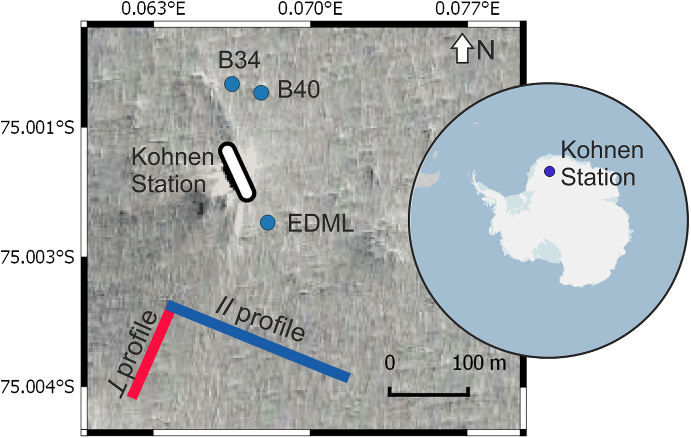
Fig. 1. Overview of the study area at Kohnen Station in Antarctica (see overview map), including the location of firn cores B40, B34 and the deep ice core EDML (blue dots) and the spread of the geophone line of the parallel to the ice divide ∥ (blue) and perpendicular to the ice divide ⊥ (red) profile. The satellite image in the background shows the surrounding area of Kohnen Station (image source: Mapcarta (2018)).
Seismic-data acquisition
To excite seismic waves we used an electrodynamic vibrator system, ElViS III P8 for the P-wave mode and ElViS III S8 for the S-wave mode. To generate the two possible polarizations of S-waves (horizontal- and vertical shear wave (SH- and SV-wave)) we rotated ElViS III S8. First, ElViS III S8 was oriented parallel to the geophone line with wave excitation perpendicular to it. The particle motion at the deepest point of the diving wave will then be in the horizontal plane and perpendicular to the geophone line and we will refer to this wave as SH-wave. Second, ElViS III S8 was oriented perpendicular to the geophone line with wave excitation parallel to it. The particle motion at the deepest point of the diving wave will then be parallel to the geophone line and we will refer to this wave as SV-wave.
ElViS III has a peak force of ~450 N and a weight of 130 kg (including batteries used as hold-down weight). The source signal consisted of a linear upsweep, over a 10 s time period with P-wave frequencies between 30 and 240 Hz and S-wave frequencies between 40 and 300 Hz. A 0.5 s taper function was applied at the start and the end of the sweep. Data were acquired at a sample interval of 0.25 ms, triggered by ElViS source control, using three-component (3-C) spiked 40 Hz geophones produced by Geospace Technologies. In total two profiles perpendicular to each other were acquired. The profiles were acquired parallel and perpendicular to the ice divide and therefore approximately perpendicular and parallel to the ice flow. The profile taken parallel to the ice divide (from now on referred to as parallel profile, indicated by symbol ∥) had a total length of 420 m. The geophones as well as the shot points in this profile had a spacing of 10 m, with the shot positions placed centred between two geophones. The arrangement of ten additional shot points beyond the geophone line results in a maximum offset of 325 m. In total, 43 shot points were occupied. At each shot location of the parallel profile, two sweeps with alternating polarity were generated for the SH-wave and SV-wave, respectively, and three sweeps for the P-wave.
The second profile was taken perpendicular to the ice divide (from now on referred to as perpendicular profile, indicated by symbol ⊥). For the P-wave mode it had a length of 115 m with a geophone spacing of 5 m while the shot spacing was 1 m, which resulted in 116 shot points. Shot locations of the P-wave mode were only placed within the geophone line, resulting in a maximum offset of 85 m. For the SH-wave mode the geophones were spaced with 10 m distance and a shot was taken every 3.3 m. No data were acquired in SV-wave mode for the perpendicular profile.
Profile locations were chosen based on proximity to the firn and ice cores, but to minimise surface disturbance on and around the Kohnen station. These profiles lie within lines of another seismic survey acquired in the Antarctic summer season 2012/13 and radar data acquired around Kohnen station. Analysis of the radar data by Eisen and others (Reference Eisen, Rack, Nixdorf and Wilhelms2005) showed a rather homogeneous accumulation around Kohnen Station, so that properties acquired from the cores can be compared to properties from the seismic lines.
Seismic wave propagation in an isotropic and anisotropic medium
The isotropic elasticity tensor (Appendix Eqn (A 1)) consists of three non-zero components c 33, c 55 and c 12 = c 33 − 2c 55, while the first Lamé constant λ is defined as
 $$\lambda = c_{33}-2\mu.$$
The shear or rigidity modulus μ is given by
 $$\mu = c_{55}= v_{\rm s}{}^{2}\rho,$$
where ρ is density and v s phase velocity of the S-wave. Another elastic modulus used in this study is the bulk modulus K, given by
 $$K=c_{33}- {4 \over 3}\mu=v_{\,{\rm p}}{}^{2}\rho-{4 \over 3}v_{\rm s}{}^{2}\rho,$$
where v p is the phase velocity of the P-wave. The Poisson's ratio, ν, is the ratio of lateral contraction and longitudinal extension,
 $$\nu = {\lambda \over 2(\mu+\lambda)} = {1/2-(v_{\rm s}/v_{\rm p})^2 \over 1-(v_{\rm s}/v_{\rm p})^2}.$$
We use the measured seismic velocities to determine ν. Other elastic moduli can all be expressed in terms of the Lamé constants (Yilmaz, Reference Yilmaz2001). Under the assumption of an isotropic medium the elastic behaviour is dependent on two elastic moduli (the Lamé constants μ and λ) and independent of the direction.
In many studies, and also in glaciology, the elastic media are assumed to be isotropic, although anisotropic ice has been observed previously in seismic studies (Backus, Reference Backus1962). The wavefronts in an anisotropic medium are no longer spherical. Several publications reported on the angle dependency of seismic wave velocity, therefore recorded traveltimes, as well as englacial reflections caused by sudden changes in crystal orientation fabric (e.g. Horgan and others, Reference Horgan2008; Hofstede and others, Reference Hofstede2013; Diez and Eisen, Reference Diez and Eisen2015; Diez and others, Reference Diez2015). Diez and others (Reference Diez2014) compared bed reflections from P- and S-wave data and found a difference of up to 7% between stacking and depth-conversion velocities for P-waves and differences of up to 1% for S-waves. They stated that these differences are caused by anisotropic fabrics.
Most seismic studies are limited to transversely isotropic (TI) models, with different orientations of symmetry axes (Tsvankin, Reference Tsvankin1997). The elastic properties of a horizontally layered medium can be described as a TI medium with a vertical (VTI) symmetry axis (Backus, Reference Backus1962; Thomsen, Reference Thomsen1986; Tsvankin, Reference Tsvankin1997). The elasticity tensor for a VTI medium has five independent coefficients c 11, c 12, c 13, c 33 and c 55 (in Voigt notation; Tsvankin, Reference Tsvankin1997), leading to the elasticity tensor given by
 $${\bf c}_{{\bf ij}}^{({\bf VTI})} = {\rm }\left( {\matrix{ {c_{11}} & {c_{12}} & {c_{13}} & 0 & 0 & 0 \cr {c_{12}} & {c_{11}} & {c_{13}} & 0 & 0 & 0 \cr {c_{13}} & {c_{13}} & {c_{33}} & 0 & 0 & 0 \cr 0 & 0 & 0 & {c_{55}} & 0 & 0 \cr 0 & 0 & 0 & 0 & {c_{55}} & 0 \cr 0 & 0 & 0 & 0 & 0 & {c_{66}} \cr } } \right)$$
with c 44 = c 55, c 13 = c 23, c 11 = c 22 and c 66 = (c 11 − c 12)/2. The phase and group velocity of P- and S-waves in a VTI medium can be found in the Appendix Eqn (A 2).
Elasticity tensor from seismic data and firn-core densities
The velocity analysis of the seismic data acquired at Kohnen Station utilised a diving-wave inversion, consisting of two processing steps (Slichter, Reference Slichter1932; Kirchner and Bentley, Reference Kirchner and Bentley1990; Diez and others, Reference Diez, Eisen, Hofstede, Bohleber and Polom2013). The first step is fitting an exponential curve to offset–traveltime pairs of diving waves' first breaks (Kirchner and Bentley, Reference Kirchner and Bentley1990).
The second step is the Herglotz-Wiechert inversion, described in the paragraph below. A requirement for both processing steps is a monotonically increasing velocity with depth.
The first breaks of the diving waves were picked manually on pre-processed data, by picking the zero-crossing of the up-going part of the Klauder wavelet (Fig. 2). The pre-processing included cross-correlation of the raw data with a synthetic sweep. To prevent phase distortions during processing, no bandpass filtering was applied.
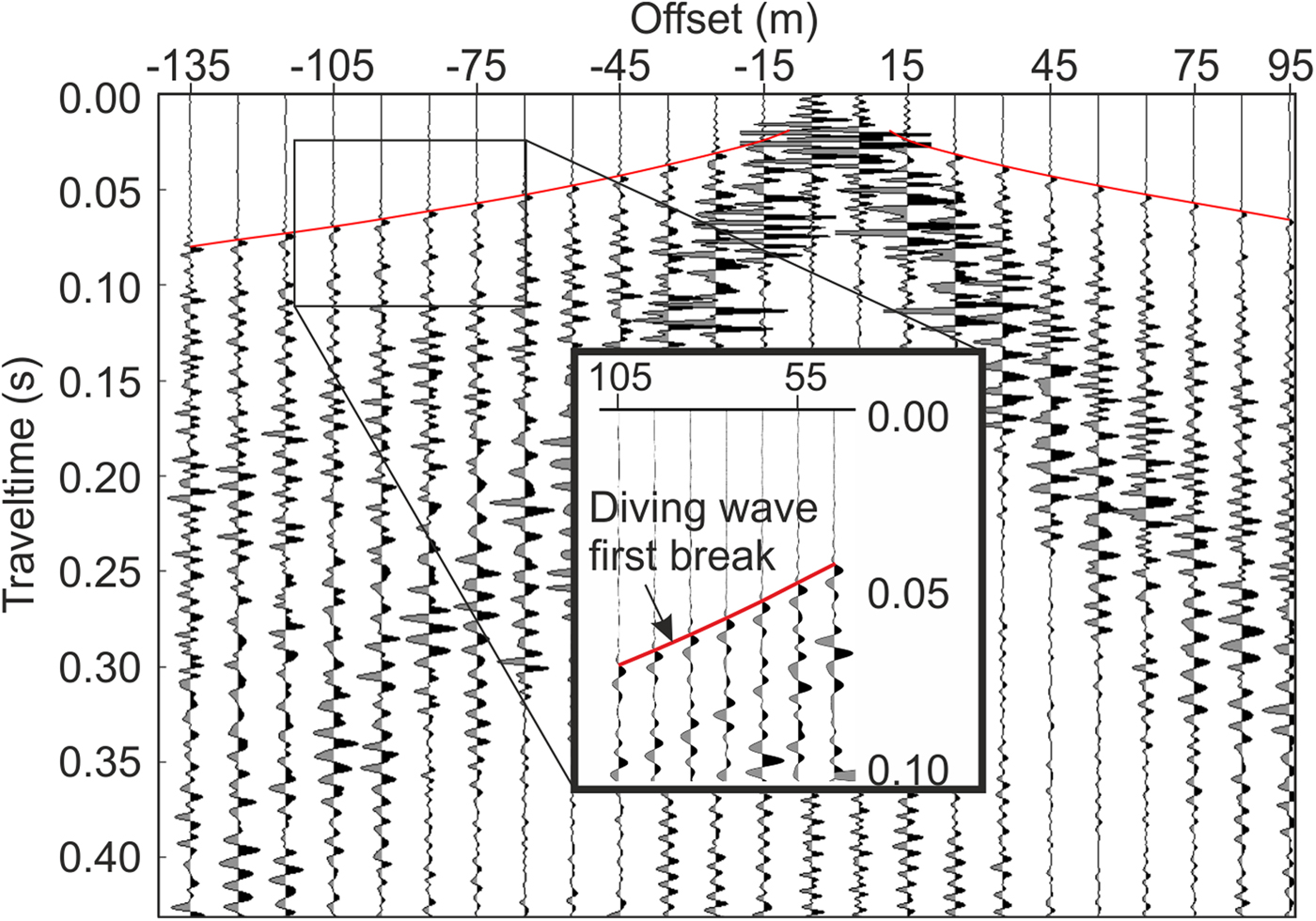
Fig. 2. Pick of the first breaks of the diving waves for the P-wave shot 60 of the parallel profile. Diving wave first arrivals have been picked on cross-correlated data at the zero-crossing of the upgoing part of the Klauder wavelet (red line).
Farrell and Euwema (Reference Farrell and Euwema1984) recommended picking the most dominant peak of the Klauder wavelet, as the Klauder wavelet is a zero-phase wavelet. The error we introduce by picking the more easily identifiable zero-crossing instead is ≤ 0.009 s. Further, the frequency for the first break is constant, so that picking the first break only introduces a constant offset within the uncertainty of our data. However, we recommend that the dominant peak should be picked in future studies using vibroseis data.
After picking the first breaks we fitted an exponential smoothing function
 $$t=a(1-\exp^{-bx})+c(1-\exp^{-{\rm d}x}) + ex,$$
to the offset–traveltime pairs using the Levenberg-Marquardt algorithm, where a, b, c, d, e are constants and t and x the traveltime and offset, respectively. The apparent velocity (v A) is then given by v A(x) = x/t. The velocity (v D) at the largest offset (D) is defined as the gradient of the offset–traveltime curve (Kirchner and Bentley, Reference Kirchner and Bentley1990):
 $$v_D={{d}x \over {d}t}.$$
Herglotz-Wiechert inversion
Diving waves are continuously refracted waves. At the deepest point of the travel path (sin(i = 90°)=1) the velocity v D at various offsets D (the gradient of this smoothed curve) is related to the inverse of the ray parameter p by
 $$v_D={1 \over p}$$
(Herglotz, Reference Herglotz1907; Wiechert, Reference Wiechert1910; Kirchner and Bentley, Reference Kirchner and Bentley1979; Nowack, Reference Nowack1990). Based on this relationship, depth values can be derived from the corresponding velocity–offset pairs. Following Slichter (Reference Slichter1932), we calculate the depth z from the corresponding velocity v D from
 $$z(v_{D})=-{1 \over \pi}\int_0^{D}(\cosh^{-1}({v_D \over v_{\rm A}(x)}))^{-1}\,{\rm d}x.$$
Firn-core density
The density distribution along the firn core was derived from radioscopic imaging of the firn core B40, performed by a 2-D XCT measurement at Alfred-Wegener-Institut, Bremerhaven (AWI). The firn core has a diameter of 0.1 m and was drilled without the use of drilling fluid during season 2012/13 to a depth of 200 m. For the 2-D XCT measurement, the sample is mounted and illuminated across the diameter of the sampling container. The transmitted radiation is captured and displayed in a greyscale-coded intensity image, from which porosity can be calculated. The vertical resolution for firn core B40 is 0.12 mm, the resulting densities have an accuracy of 2% (Freitag and others, Reference Freitag, Kipfstuhl and Laepple2013; Schaller and others, Reference Schaller, Freitag and Eisen2017). For further calculations we smoothed the firn-core density using a moving average, with a 2.5 m window. From now on the smoothed firn-core density is referred to as firn-core density.
Calculation of velocities from firn-core densities
Kohnen and Bentley (Reference Kohnen and Bentley1973) investigated the dependency of seismic velocities on temperature, anisotropy and density from seismic data acquired in 1970/71 near New Byrd Station in West Antarctica. The empirical formula by Kohnen (Reference Kohnen1972), stating a relation between density and P-wave velocity, was developed on the basis of these measurements. The atmospheric conditions (low air temperature, low accumulation, location of FIT) as well as firn structure and properties at Kohnen Station and New Byrd Station are expected to be comparable; therefore, we use the empirical formula of Kohnen (Reference Kohnen1972) to calculate P-wave velocities from densities:
 $$\rho (z) = \displaystyle{{\rho _{{\rm ice}}} \over {1 + {[(v_{{\rm p},{\rm ice}}-v_{\rm p}(z))/2250\; {\rm m}{\mkern 1mu} {\rm s}^{{\rm - 1}}]}^{1.22}}},$$
where ρ(z) is the density in the unit of kg m−3 and v p,ice are the P-wave velocities in ice in the unit of m s−1. The density–depth profile was also used to calculate S-wave velocities based on a formula stated by Diez and others (Reference Diez2014) for S-wave velocities:
 $$\rho (z) = \displaystyle{{\rho _{{\rm ice}}} \over {{\rm 1 + }{[(v_{{\rm s},{\rm ice}}{\rm - }v_{\rm s}(z)){\rm /950}\,{\rm m}{\mkern 1mu} {\rm s}^{{\rm - 1}}]}^{{\rm 1}.{\rm 17}}}},$$
where v s,ice are the S-wave velocities in ice in the unit of m s−1. We adopted ρice as suggested by Kohnen (Reference Kohnen1972) as 915 kg m−3. Elastic moduli, such as the bulk modulus, shear modulus and Poisson's ratio were calculated under the assumption of an isotropic medium using Eqns (2)–(4). In order to avoid uncertainties induced by converting velocities into densities we used measured firn-core densities.
Elasticity tensor from firn-core samples: 3-D structural data
Microstructural data were obtained from 3-D XCT. Here, the sample is illuminated from different angles, in contrast to the 2-D XCT measurement, to derive firn-core densities. The plate on which the sample is mounted rotates in a certain interval while the detector moves in vertical steps during scanning. More than 32 000 shadow images are captured during sampling one depth interval, which are then transformed into a series of horizontal cross-sections by a digital convolution algorithm. These represent the 3-D structure of the object based on the local differences in X-ray absorption (Freitag and others, Reference Freitag, Wilhelms and Kipfstuhl2004). The 3-D structural data were obtained for a sample volume of 12 × 12 × 12 mm3 at four different depths (10, 42, 71, 99 m) from the core B34 at the AWI.
The elasticity FEM code for voxel-based microstructure provided by the National Institute of Standards and Technology (Garboczi, Reference Garboczi1998) was employed (Srivastava and others, Reference Srivastava, Chandel, Mahajan and Pankaj2016; Gerling and others, Reference Gerling, Löwe and van Herwijnen2017). In the FEM code, isotropic elastic material properties are assigned to the two constituents (air and ice) to numerically solve the equations of linear elasticity in the heterogeneous material. The components of the homogenized elasticity tensor are given by the linear relations between volume averaged stresses and strains.
For the FEM we used the bulk and shear moduli G = 3.52 GPa and K = 8.9 GPa of polycrystalline ice (Schulson and Duval, Reference Schulson and Duval2009) to compute the components c 11, c 33, c 55, c 12, c 13 of the elasticity tensor for a transversely isotropic (TI) medium at the four depths at which 3-D XCT data was measured. Further details on the elastic homogenization problem can be found in Torquato (Reference Torquato2002). As no values could be determined from the seismic data for the deepest sample at 99 m, we focus on the three shallower sampling depths. For the comparison of the moduli from FEM and diving waves, we calculated an estimate of the bulk and shear modulus from the full elasticity tensor according to Eqns (1)–(4).
RESULTS
Offset–traveltime picking
We picked P- and S-wave offset–traveltimes for all data along the parallel and perpendicular profile. The offset–traveltime pairs of the perpendicular profile showed substantial scattering (±0.006 s), which increased the uncertainty of calculated moduli. We therefore discarded the results of the perpendicular profile in the following and focus on results and discussion of data from the parallel profile.
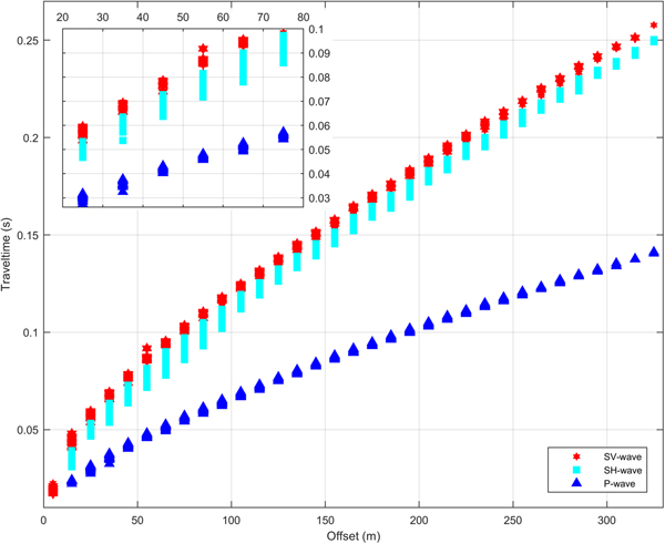
We find no traveltime differences between shots from the western and eastern ends of the profiles. The SV-wave shows smaller traveltimes compared to the SH-wave traveltimes, with a maximum time difference of 20 ms (20%) for an offset of 75 m (~15 m depth) and a maximum difference of 8 ms (3%) for the maximum offset of 325 m (~75 m depth). The fit of the exponential curve Eqn (6) to the offset–traveltimes converged for each wave type, irrespective of using traveltimes from all locations as well as using traveltimes from individual shots for all three wave types.
Seismic velocities
The calculated velocities for both wave types (P- and S-wave) increase continuously with depth (Fig. 4). P-wave velocity (blue solid line) increases from 2000 m s−1 at 10 m depth to 3400 m s−1 at 77 m depth. The P-wave velocities from diving waves and from velocities calculated using the empirical formula from Kohnen (Reference Kohnen1972, Eqn (10)) applied to firn-core densities, (black dashed line) deviate by 2% at 70 m depth.
SH- (cyan solid line) and SV-wave velocities (red solid line) increase from 1250 m s−1 at 10 m depth to 1700 m s−1 at 77 m depth. A difference in SH- and SV-wave velocities can be observed with a maximum difference of 140 m s−1 (16%) at a depth of 4.5 m and a difference of 41 m s−1 (2.5%) at a depth of 40 m. We compare this to S-wave velocity calculated from firn-core densities using Eqn (11; Diez and others, Reference Diez2014) (black solid line). The difference amounts to 26% at a depth of 10 m and a difference of 0.5% at a depth of 70 m.

Fig. 3. Distribution of all picked offset–traveltime values for the different wave types of the parallel profile. Inset shows a zoom on the offset–traveltime pairs from the shallow firn.
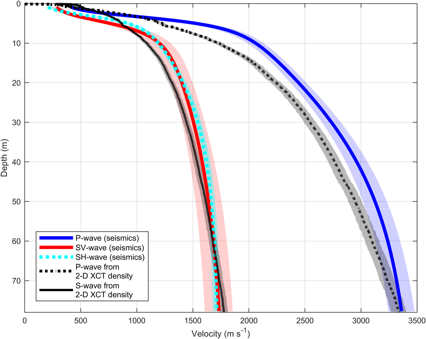
Fig. 4. Velocity–depth profile from seismic data and smoothed firn-core densities converted into seismic velocities using empirical formulas described in the main text. Shaded area in the background displays the range of uncertainties. Uncertainty is calculated by incorporating the picking uncertainty, fitting uncertainty and the uncertainty from firn-core density measurements, as described in the main text.
Elastic moduli
Elastic moduli from diving-wave inversion and firn-core densities
The densities obtained by 2-D XCT measurements from the firn core B40 down to a depth of ~90 m show small-scale density variations (10–15%, Fig. 5, see grey coloured values in the background).
At 87 m depth the density is 830 kg m−3 (2% uncertainty), which corresponds to the critical density for the FIT zone. Figure 6 shows the calculated bulk and shear moduli using P- and SH-wave velocities from diving-wave inversion and firn-core densities.
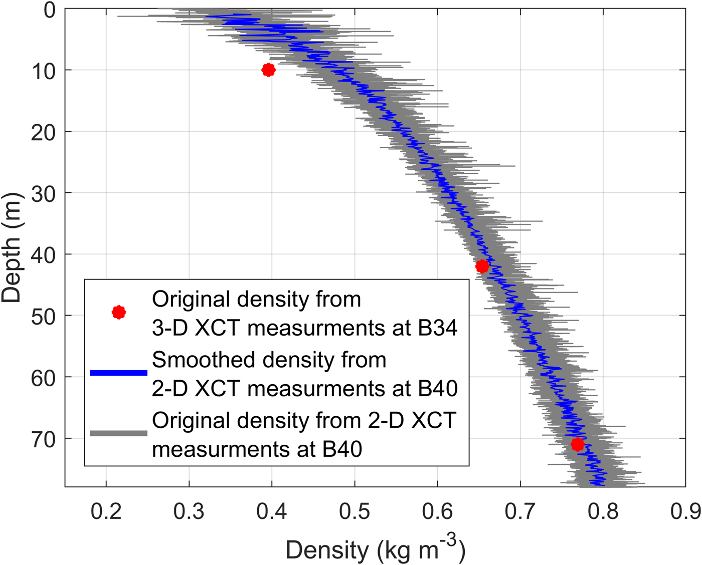
Fig. 5. Density–depth profile derived from 3-D XCT point measurements (red) and quasi-continuous radioscopic 2-D XCT measurement (blue). The blue line shows the smoothed density data (moving average with a window of 2.5 m), with the original data shown in grey in the background.
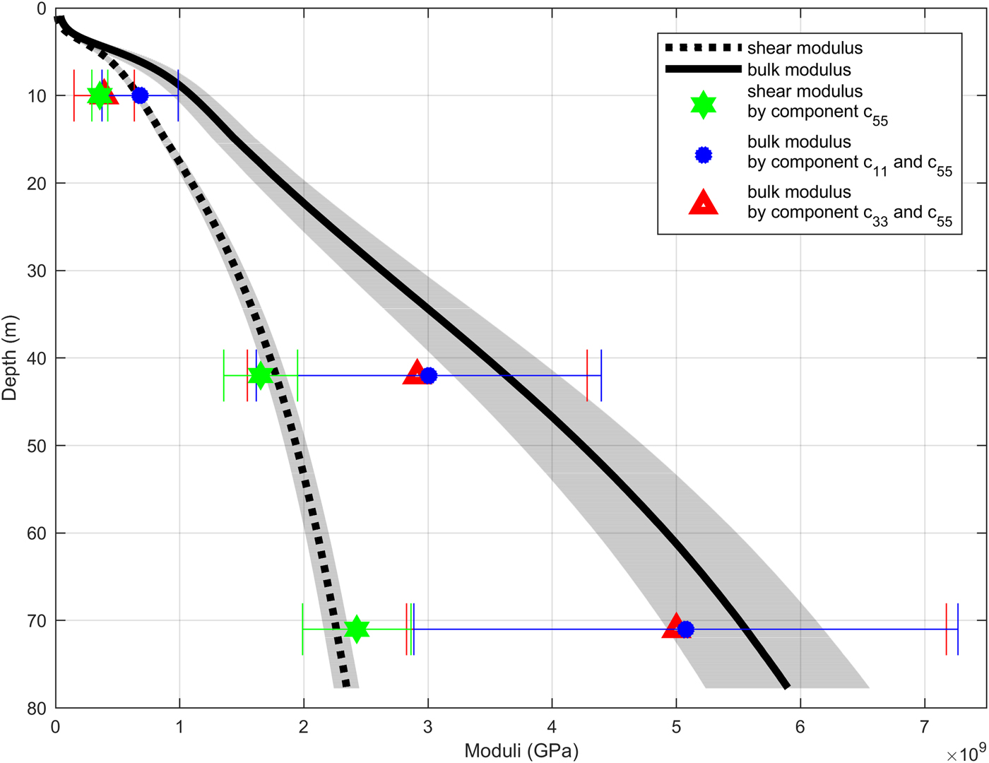
Fig. 6. Bulk (black solid line) and shear modulus (black dashed line) derived from diving-wave inversion combined with the firn-core densities. Red triangles and blue dots represent the bulk modulus derived from the components of the elasticity tensor c 33 and c 11, respectively. Green stars represent the shear modulus derived from the component of the elasticity tensor c 55. Shaded area in the background displays the range of uncertainties of the diving wave velocities. Error bars display the uncertainty range of FEM derived bulk and shear moduli. Calculated values for bulk and shear moduli, poisson's ratio and densities derived from 3-D XCT measurements and FEM are tabulated in Table 1 for comparison.
Table 1. Values from 3-D XCT and FEM for 10, 42 and 71 m depth. The values are displayed in Fig. 5, Fig. 6, Fig. 7
The shear modulus μ calculated from velocities inverted from SH-diving waves and firn-core densities increases from 0.66 GPa at 10 m depth to 2.35 GPa at 77 m depth (black dashed line, Fig. 6). The bulk modulus K calculated from firn-core densities and P-wave velocities from diving-wave inversion and shear modulus increases from 1.12 GPa at 10 m depth to 5.8 GPa at 77 m depth. The bulk moduli K and shear moduli μ calculated using SH- and SV-wave velocities differ only slightly (<5%), therefore, we do not investigate their difference further.
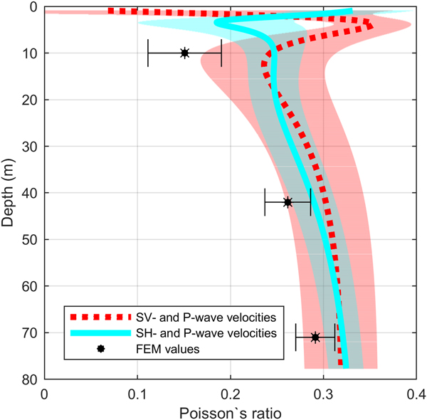
Poisson's ratios derived from seismic velocities is shown in Figure 7. The Poisson's ratio derived from SH- and P-waves (cyan solid line) increases from 0.247 at 10 m depth to 0.32 at 71 m depth, and for the SV- and P-wave (red dashed line) from 0.241 to 0.318, respectively.

Fig. 7. Comparison of Poisson's ratio derived from SH- and P-wave data (cyan solid line) and SV- and P-wave data (red dashed line). Black stars display FEM derived Poisson's ratio. Coloured area in the background displays the range of uncertainty of the diving wave velocities. Error bars display the uncertainty range of FEM derived Poisson's ratio.
Elastic moduli derived from FEM
Bulk and shear moduli calculated by the FEM derived components of the elasticity tensor are shown in Figure 6. The shear modulus derived from the component c 55 (green star) of the elasticity tensor in 10 m depth is 0.36 GPa and increases to 2.43 GPa at 71 m depth. A difference in bulk moduli derived from the components of the elasticity tensor c 33 (red triangle) and c 11 (blue dot) can be seen (Fig. 6). The bulk modulus derived from the component c 33 of the elasticity tensor in 10 m depth is 0.68 GPa whereas the bulk modulus derived from the component c 11 is 0.39 GPa. The difference between the two components decreases with depth to a minimum of 0.4%. The Poisson's ratio (Fig. 7) calculated using the components c 11 and c 55 (black star) of the elasticity tensor in 10 m depth is 0.15 and increases to 0.29 at 71 m depth.
Uncertainty ranges
The coloured area in the background of Figs 4, 6 and 7 indicates the uncertainty range of the calculated velocities, bulk and shear modulus and the Poisson's ratio, respectively, derived from seismic data. For moduli calculated from firn-core densities and seismic velocities the uncertainty is calculated using a 1-σ error band for the offset–traveltimes (2 ms), the uncertainty of fit of the exponential function to the offset–traveltimes (1-σ confidence bounds) and the uncertainty of the firn-core densities (2%). These uncertainty ranges were then incorporated into Gaussian error propagation. The uncertainty for seismic velocities calculated from firn-core densities is limited to the uncertainty of the 2-D XCT measurement of 2%. Uncertainties caused by the application of the Kohnen (Reference Kohnen1972) and the Diez and others (Reference Diez2014) formula to calculate velocities are not taken into account.
Traveltimes were only picked for offsets larger than 15 m for both wave types. Velocities calculated from diving waves for depths <10 m should not be considered, since these velocities are not based on measurements but on the fitted curve. Due to the scattering of the data, the uncertainty in shallow depth might be underestimated and care has to be taken when comparing the values to other data.
Error bars for the point values in the background of Figs 6 and 7 indicate a 1-σ uncertainty range for shear, bulk modulus and Poisson's ratio, respectively, derived from FEM. The uncertainty of these values depends on the uncertainty of the elastic properties in ice, assumed for the FEM, uncertainties in the segmentation and spatial variations in density. Gerling (Reference Gerling2016) investigated the uncertainty of the elasticity tensor and postulates a maximum uncertainty of 18.2% for the component c 33. This uncertainty was adopted for the other elasticity tensors as well since all were derived from the same FEM. Due to error propagation the error for the bulk modulus calculated from FEM values amounts to 42%. A better individual uncertainty for the components of the elastic tensor could only be obtained by the estimation and incorporation of lateral density variations and more accurate segmentation, for instance by analysing more sample segments in one depth.
DISCUSSION
Seismic velocities from firn-core densities and potential effect of anisotropy
The comparison of P-wave velocities calculated from diving waves and velocities calculated using firn-core densities and the Kohnen (Reference Kohnen1972) formula show a good fit (Fig. 4, 2% difference in 70 m depth). The same holds for the S-wave velocities from diving waves in comparison with velocities calculated with the relation postulated by Diez and others (Reference Diez, Eisen, Hofstede, Bohleber and Polom2013).
The differences between SH- and SV-wave traveltimes (Fig. 3), thus SH- and SV-wave velocities (Fig. 4), indicate anisotropy. At the deepest point of the ray path, where the wave bends upwards, the SH-wave particle motion oscillates purely in the horizontal plane, while the SV-wave induces a particle oscillation in the vertical plane, i.e. perpendicular to the SH-wave (Wendt, Reference Wendt and Bormann2002). In our case the particle velocity in the radial direction is faster than in the tangential direction (V SV > V SH), a difference in SH- and SV-wave velocity which is referred to as S-wave anisotropy (Bale and others, Reference Bale2009). The elastic moduli were calculated under the assumption of an isotropic medium, which is certainly not correct for firn. Indications for anisotropy in firn were for instance investigated by Fujita and others (Reference Fujita, Okuyama, Hori and Hondoh2009) based on measurements of relative dielectric permittivity, bulk density, 3-D pore space structure and crystal-orientation fabric of firn at Dome Fuji (East Antarctica). They found that the relative dielectric permittivity of the analysed samples was always greater or the same in the vertical component compared to the horizontal component. Furthermore, they determined a slight structural anisotropy within the firn.
Seismic anisotropy in firn can have different causes: (i) a structural anisotropy, (ii) an effective anisotropy and (iii) an intrinsic anisotropy. Structural anisotropy is caused by a preferred direction in the structure of the snow and firn matrix. This anisotropy can be determined by different methods due to the impact on thermal, dielectric or mechanical properties (Löwe and others, Reference Löwe, Riche and Schneebeli2013; Leinss and others, Reference Leinss2016; Srivastava and others, Reference Srivastava, Chandel, Mahajan and Pankaj2016). In case of isotropy, the component c 33 (derived from the FEM) equals the component c 11 as well as the component c 12 equals the component c 13 of the elasticity tensor. In our case this assumption seems not to be valid, since the components c 33 and c 11 derived from FEM differ by more than 33% at a depth of 10 m and <2% for the other measurements.
The effective bulk anisotropy is an anisotropy caused by layers with varying density and Lamé constants, i.e. layers with varying seismic velocities significantly thinner than the seismic wavelength (Backus, Reference Backus1962). The seismic wave experiences an effective, averaged medium due to the wavelength being significantly larger than the layer thickness. This leads to different effective elastic properties in vertical and horizontal direction and thus to an effective seismic anisotropy. This effective anisotropy due to thin layers was observed previously at the Ross Ice Shelf (Diez and others, Reference Diez2016). At Kohnen station the firn density varies as much as ±80 kg m−3 on a mm-scale (Hörhold and others, Reference Hörhold, Kipfstuhl, Wilhelms, Freitag and Frenzel2011; Freitag and others, Reference Freitag, Wilhelms and Kipfstuhl2004). These variations cause an effective bulk anisotropy.
The intrinsic anisotropy is an anisotropy caused by a preferred orientation of the anisotropic, hexagonal ice crystals and has been observed in seismic data previously (Picotti and others, Reference Picotti, Vuan, Carcione, Horgan and Anandakrishnan2015). The intrinsic anisotropy develops due to the stresses within the ice, which are comparatively small within the firn. Hence, the intrinsic anisotropy is expected to increase with depth as has been observed in ice cores (Montagnat and others, Reference Montagnat2014). We therefore assume that the intrinsic anisotropy is small within the firn column compared to the structural and effective anisotropy. Furthermore, we expect a decrease in the strength of the anisotropy with depth for the structural and effective anisotropy, which is caused by variations and structures within the firn that decrease with depth and the transformation from firn to ice. Attributing the observed anisotropy to a structural and effective anisotropy explains the observed difference between the values derived from seismic diving waves and the FEM with depth. The observed decreasing difference between the components c 33 and c 11 derived from FEM can be explained by decreasing structural anisotropy with depth.
Given the pilot character of our study for this type of investigation, we refrain from further analysing the overall effect of anisotropy on the data. Nevertheless, a refined set-up and careful deployment of seismic-data acquisition has the potential to identify anisotropic properties in the firn from the surface, as presented by Picotti and others (Reference Picotti, Vuan, Carcione, Horgan and Anandakrishnan2015). Using a factorised velocity model, for example comparable to the one described by Xu and others (Reference Xu, Stovas and Alkhalifah2016), anisotropy parameters can be determined. The isotropic velocity model (acquired from diving waves under the assumption of an isotropic medium) could thus be corrected for effects of a VTI medium. In our approach we assumed isotropy using the Herglotz-Wiechert inversion to analyse the data. Our results then show anisotropy within the firn. Hence, an error is introduced using the Herglotz-Wiechert inversion for isotropic material. In future this should be taken into account and an inversion scheme for diving waves in anisotropic material needs to be developed.
Comparison of elastic moduli
The method introduced by Gerling and others (Reference Gerling, Löwe and van Herwijnen2017) is the same as used here. They found that the elastic moduli derived from acoustic wave propagation are in agreement with the moduli derived from FEM (within the uncertainty range), as long as the Backus effect is taken into account. If neglected, FEM moduli are larger than their acoustic counterparts. In contrast to this, our results from the FEM have lower elastic moduli compared to the elastic moduli derived from seismic velocities (within the given range of uncertainties).
There are two possible reasons for these differences. First, the seismic wavelength used in our study (10 m) is large compared to Gerling and others (Reference Gerling, Löwe and van Herwijnen2017; 1.5–5 cm calculated for a frequency of 15 kHz and a wave speed of 230–850 m s−1) and this might influence the obtained elastic moduli (Marion and Coudin, Reference Marion and Coudin1992; Fjær, Reference Fjær2009). Secondly, our methods have different resolution. Figure 5 shows the densities from the 2-D XCT measurement and densities of the point measurement of the 3-D XCT measurement. Both have the same vertical resolution but a different horizontal resolution since the 3-D XCT illuminates the sample from different angles. The first two values of the 3-D XCT measurement (at 10 m and 42 m depth, Fig. 5) lie within an area of 15% density variation and represent a layer with a lower density compared to the layer above and below. We therefore consider this sample not to be fully representative of the mean properties at this depth range. In contrast, according to the 2-D XCT densities, the 3-D XCT density at a depth of 71 m is representative for this depth. This is also seen in the shear modulus derived for the components of the elasticity tensor, which agree with the shear modulus derived from seismics and firn-core densities within 7.8% (Fig. 6). The minimum seismic wavelength within the firn in our survey is roughly on the order of 10 m. Therefore, no individual layer but the average of properties within a 2.5 m column (which equals a quarter of the seismic wavelength) affect the seismic wave propagation. For further studies of this type, where the objective is to compare results from high-resolution firn-core structure with seismic data and 3-D XCT measurements, we recommend to first evaluate the density profile to make sure that the sample for the 3-D XCT measurement consists of a layer that is representative for the considered depth, as has been done by Gerling and others (Reference Gerling, Löwe and van Herwijnen2017).
The fact that the calculated elastic moduli fall within the uncertainty range of the FEM elastic moduli shows that diving waves are a useful method in combination with independent density estimates to derive reasonable elastic moduli. Deriving elastic moduli from diving waves is, compared to deriving elastic moduli using firn cores and the FEM, an excellent method to gain information in an efficient manner and beyond the location of the firn core, and involves lower uncertainties.
To achieve higher accuracy within the upper meters of the firn we recommend a modified acquisition geometry. A logarithmically increasing near-offset range would sample diving waves from the first few meters of the firn as well as from greater depth.
CONCLUSIONS
We successfully combined a dynamic method to acquire diving waves, and thus seismic velocities, and a static method to measure densities and components of the elasticity tensor. With this study we demonstrate that elastic moduli can be accurately determined using diving waves and firn-core densities. The elastic moduli derived from seismic-data analyses are within the range of uncertainties of the elastic moduli obtained from the FEM approach, in particular below a depth of ~10 m in the firn. Nevertheless, at the present degree of accuracy we cannot exclude that a systematic difference between the dynamic and static moduli, as observed in geomechanical literature, is still present. We cannot finally conclude whether the differences in velocities and elastic moduli calculated from differently polarised S-waves are caused by structural anisotropy in firn or not. Nevertheless, the visibility of the effects of seismic shear-wave anisotropy shows that the high-resolution vibroseis method with a defined source polarisation from the surface has a distinct advantage to determine elastic properties in firn over methods with less repeatable seismic source characteristics as obtained from hammer or explosive sources.
The performance of the 3-D XCT as well as the FEM is time consuming, whereas the analysis of firn-core density and diving-wave inversion can be achieved faster. As the latter analyses also represent rather spatially continuous values for the elastic moduli (with the limitation of values of density) in contrast to the local point measurements of elastic moduli from the FEM, the additional effort for seismic-data acquisition in the field is partly compensated. To overcome the need for firn-core retrieval to convert seismic velocities to elastic moduli, one could also envisage using common midpoint surveys with ground-penetrating radar as an independent source of a density–depth distribution (Arthern and others, Reference Arthern, Corr, Gillet-Chaulet, Hawley and Morris2013). Although those will still be obtained at higher resolution than the seismic velocities, the smoothing of radar-wave propagation will reduce the effect from layers with a particularly different density.
ACKNOWLEDGMENTS
Preparation of this work was supported by the Emmy Noether program of the Deutsche Forschungsgemeinschaft grant EI 672/5 to O.E. Discussions with G. Druivenga and U. Polom during vibroseismic survey design and analyses facilitated this study. We greatly acknowledge the assistance of AWI's logistic personnel at Kohnen station without whom the data acquisition would not have been possible. Finally, we are grateful for comments of the reviewers A. Brisbourne and G. Stuart, as well as the editor B. Kulessa that helped to improve the manuscript.
APPENDIX A.
A.1. Elastic moduli
The elasticity tensor for an isotropic medium is given as follows:
 $${\bf c}_{{\bf ij}}^{({\bf iso})} = \left( {\matrix{ {c_{33}} & {c_{12}} & {c_{12}} & 0 & 0 & 0 \cr {c_{12}} & {c_{33}} & {c_{12}} & 0 & 0 & 0 \cr {c_{12}} & {c_{12}} & {c_{33}} & 0 & 0 & 0 \cr 0 & 0 & 0 & {c_{55}} & 0 & 0 \cr 0 & 0 & 0 & 0 & {c_{55}} & 0 \cr 0 & 0 & 0 & 0 & 0 & {c_{55}} \cr } } \right){\rm }$$
with c 11=c 22=c 33= 2μ + λ, c 44 = c 55 = c 66 = 2μ and c 12 = c 21 = c 13 = c 31 = c 23 = c 32 = c 33 − 2c 55 = λ (Yilmaz, Reference Yilmaz2001).
In a VTI medium the phase and group velocity of P- and S-waves are defined as follows:
 $$\eqalign{& v_{\rm P}(\theta = 0) = \sqrt {\displaystyle{{c_{33}} \over \rho }} , \cr & v_{\rm SH}(\theta = 0) = \sqrt {\displaystyle{{c_{55}} \over \rho }} , \cr & v_{\rm SV}(\theta = 0) = \sqrt {\displaystyle{{c_{55}} \over \rho }} , \cr & v_{\rm P}(\theta = 90) = \sqrt {\displaystyle{{c_{11}} \over \rho }} , \cr & v_{\rm SH}(\theta = 90) = \sqrt {\displaystyle{{c_{66}} \over \rho }} , \cr & v_{\rm SV}(\theta = 90) = \sqrt {\displaystyle{{c_{55}} \over \rho }} .}$$
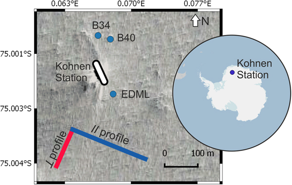


 Open access