


1. Introduction
The Earth’s ice sheets are of strong scientific interest (Reference SolomonSolomon and others, 2007). Improved remote monitoring underneath ice sheets would be useful for a number of reasons. For example, such monitoring would allow a better understanding of glacial motion at the ice-sheet bed, which helps determine ice fluxes to the ocean, ice-sheet mass balance and sea-level change (Reference Engelhardt, Humphrey, Kamb and FahnestockEngelhardt and others, 1990; Reference Rignot and ThomasRignot and Thomas, 2002). Water flow at the ice-sheet sole has an important influence on glacial motion via its effect on the friction between the ice sheet and the underlying sediments (Reference BellBell, 2008; Reference Winberry, Anandakrishnan, Wiens, Alley and ChristiansonWinberry and others, 2011). Also, subglacial environments are a viable habitat for microbial life (Reference Sharp, Parkes, Cragg, Fairchild, Lamb and TranterSharp and others, 1999; Reference Skidmore, Foght and SharpSkidmore and others, 2000; Reference FoghtFoght and others, 2004), despite the low temperatures and scarcity of food and energy sources. Subglacial lakes and sub-ice-stream sediments house significant populations of microorganisms which are adapted to the lack of sunlight, low temperature and sparsity of nutrients/organic carbon (Reference PriscuPriscu and others, 1999; Reference LanoilLanoil and others, 2009). These environments are a unique component of the Earth’s biosphere, and may play a key role in the Earth’s biogeochemical cycles (Reference SiegertSiegert and others, 2001; Reference WadhamWadham and others, 2010). Basal drainage is also a control on, for example, glacier surging (Reference BjörnssonBjörnsson, 1998), so monitoring is broadly relevant for glaciologists. Local subglacial monitoring offers the possibility of rapid scientific advance via the acquisition of high-temporal-resolution in situ datasets. However, the current understanding of subglacial processes is limited: difficulties of access, low temperatures, high pressure and abrasion limit in situ process measurements. This paper discusses the potential for acoustic communication of data from such measurements.
Deploying sensors beneath the ice sheets presents an engineering challenge, because the environment to be monitored is hostile and difficult to access. The Antarctic ice sheet ranges in thickness from hundreds of metres near the coast to 4 km in the centre (Reference Anandakrishnan and WinberryAnandakrishnan and Winberry, 2004). The Greenland ice sheet rises to >3km thickness (Reference Bamber, Layberry and GogineniBamber and others, 2001). At these thicknesses the base of the ice sheet is only accessible via expensive and time-limited drilling programmes, and the pressures, complex stresses and abrasion experienced by any sensor at the bed may be extreme. The ice moves by several metres per year in the interior of the ice sheets and on the order of 1 km a–1 in fast-moving ice streams (Reference BentleyBentley, 1987), which means that any tethered probe has a limited lifetime and in many cases is impractical.
Monitoring of the basal regions of ice sheets from the surface is typically conducted via radar (Reference Siegert, Carter, Tabacco, Popov and BlankenshipSiegert and others, 2005; Reference Woodward and BurkeWoodward and Burke, 2007) and acoustic techniques (Reference Anandakrishnan, Blankenship, Alley and StoffaAnandakrishnan and others, 1998). These, therefore, seem likely technologies for through-ice communications. Wireless devices offer the possibility of long-term local sensing, but present their own problems. Typical renewable power supplies for wireless sensors (e.g. solar, wave) are unavailable beneath the ice sheet, so an internal power supply is required. In addition, data have not historically been transmitted through thick ice, hence there is no clear guide for optimization of communications. Radio communications through ice have already been attempted, with successful transmission over ranges of the order of 100m (Reference Padhy, Martinez, Riddoch, Ong and HartPadhy and others, 2005) to 2500 m of dry, cold ice (Reference SmeetsSmeets and others, 2012). However, once the sensor is located in a wet environment (e.g. subglacial lake, water-saturated sediments, conduits or simply temperate ice), high radio attenuation in water limits communication to ranges of a few metres (hence the use of sonar for maritime communications). Many environments of interest (e.g subglacial lakes and ice streams) require communication through 10–100 m of water or wet sediments. Hence we focus here on an assessment of the feasibility of data transmission using acoustic techniques. Acoustic communications are well established. For example, fax machines send data over standard telephone lines.
We begin by considering the four major types of polar environment, summarized in Figure 1, from which one might wish to communicate data wirelessly. Data transmission may be required from a wireless sensor in any of the following scenarios:
-
1. embedded in ice (where a small local melt layer of several millimetres may be created by heat emitted from the device);
-
2. in a subglacial lake, where the acoustic energy is coupled directly into a large body of water;
-
3. buried in a water-saturated till layer (e.g. at the bed of an ice stream); or
-
4. buried in subglacial sediment beneath a subglacial water body (i.e. a combination of (2) and (3)).

Fig. 1. Schematic of transmission paths beneath an ice sheet (not to scale). Likely deployment scenarios include (a) transmitter embedded in ice, surrounded by local melt layer; (b) transmitter sits on base of subglacial lake; (c) transmitter buried in subglacial sediment; (d) transmitter buried in subglacial lake sediment.
We evaluate the potential for acoustic communications in each of these environments in turn, commencing with an evaluation of the general requirements for collecting data beneath the ice sheet and communicating them to the surface.
2. System Requirements
A system which can access, survive and transmit data from the four scenarios of Figure 1 must meet several design criteria. In concept the system should act as a subglacial oneway data conduit, such that data from any low-power sensor (e.g. pressure or pH sensors) can be logged, and the results relayed to the ice-sheet surface. One fairly simple initial application of the probe (i.e. the entire subglacial package of sensors and communications) would be to transmit local temperature and pressure, to better understand subglacial drainage characteristics and water flow over the ice-sheet bed. A more complex probe might measure the chemical and biological properties of in situ meltwaters, giving information about the subglacial biota and their activity.
Deep subglacial deployment is only possible via boreholes drilled through the ice cover, which limits the size of the probe and hence the available power supply. Typical borehole sizes are ∼100 mm, as used for ice coring, allowing a device of a few centimetres diameter; thus, a cylindrical device might allow an internal volume of the order 1 L (e.g. the WiSe (Wireless Sensor) project (Reference SmeetsSmeets and others, 2012), which deployed a radio transmitter package down the NEEM borehole in central Greenland, details a deployed internal volume of 1.5 L). Beneath the ice the probe may be subject to pressures above 100MPa and severe abrasion, so the physical structure will need to be robust, with a thick outer shell. The internal cavity is shared between instrumentation, power, communications and associated electronics. Typical energy densities for lithium ion technology are ∼1MJL–1 (this may be reduced with current self-discharge and at low temperatures). The total available stored energy is therefore of the order of 1 MJ. The available signal power is likely to be limited by acoustic cavitation at the transducer or by efficiency considerations. For now, we consider an available electrical power output of 1 W; later we will discuss the merits of varying the power output.
Successful communication of data from the ice-sheet bed to the ice-sheet surface depends on the signal-to-noise ratio (SNR) at the receiver. The signal strength at the receiver depends on the transmitted signal strength and the power lost along the transmission path. Power is lost due to:
-
transducer losses in converting electrical energy to acoustic energy at the source
-
coupling losses in transmitting acoustic energy from the source to its surrounding medium
-
path loss due to beam spreading
-
signal reflections at interfaces in transmission media
-
signal attenuation within media.
These components can be combined into a link budget, in which the lost signal power is summed and the received power predicted.
where P R is received power and P T is transmitted power (measured in dB m, i.e. relative to 1 mW), P is path loss, A is the attenuation loss in the transmission media, R is the reflection loss at the interfaces between media, T is transducer loss and C is the coupling loss (all measured in dB).
In the next section we discuss signal attenuation, with reference to new field experiments. We then present estimates of the other losses in the transmission path, and noise at the receiver. Finally we present these values in the context of Eqn (1), to estimate the range of acoustic communication from a subglacial transmitter.
3. Signal Attenuation
3.1. Attenuation in relevant transmission media
When sound propagates through any medium, the signal energy is reduced due to a combination of absorption (in which the signal energy is directly converted to heat) and scattering (where the signal is deviated by non-uniformities in the medium) (Reference PricePrice, 2006). For communication, the total attenuation is critical (since it determines the received signal strength). The attenuation of acoustic waves is dependent on the transmission medium, so we consider attenuation in the three media of interest: ice, water and sediment.
3.1.1. Ice
At low temperatures, the attenuation of ice is dominated by absorption (Reference PricePrice, 2006). In bubbly or heterogeneous ice, scattering may dominate over absorption. When scattering dominates, attenuation increases with frequency (Reference PricePrice 2006). Attenuation increases with ‘temperature, impurity content, crystal size and degree of randomness of crystal orientation’ (Reference PricePrice, 1993). Because of this variability, the feasibility of acoustic communications is likely to be highly geographically dependent. Relatedly, the acoustic wave speed in ice is known to be highly dependent on air and water inclusions, which affect the bulk compressibility (Reference RöthlisbergerRothlisberger, 1972; Reference Nolan and EchelmeyerNolan and Echelmeyer, 1999).
Reference PricePrice (2006) found from preliminary analytical modelling and laboratory experiments that the predicted attenuation length (the attenuation length is the length over which the acoustic intensity is reduced by a factor of 1/e) of sound in South Polar ice (temperature -55°C, grain size 2 mm) was 9 ± 3 km at 30 kHz, with the attenuation dominated by absorption. This corresponds to a power decrease of ∼1 dB km–1 through attenuation. This value is small compared to the spreading loss, and suggests that acoustic communications through South Polar ice should have a comparable range to maritime acoustic communication, i.e. 5-10 km. In any ice that matches these experimental predictions, acoustic communications will be suitable for bed-surface data transfer.
The experimental predictions by Reference PricePrice (2006) were made to inform the IceCube project (IceCube Collaboration, 2006). As part of IceCube, the South Polar Acoustic Test Setup (SPATS) has been operational since 2007. One of the core aims of the SPATS project (IceCube Collaboration, 2011) was to measure the attenuation of sound waves in South Polar ice in the range 10-100 kHz. Measuring the attenuation length in situ, they found an attenuation length of 300 m ±20%, independent of frequency (up to 30 kHz) and depth (up to 500 m). This corresponds to power ) attenuation of ∼30dBkm–1 , significantly higher than the predictions of Reference PricePrice (2006). The authors of the SPATS report suggest that the discrepancy may be due to ice grains being larger than anticipated, so that scattering, not absorption, is the dominant attenuation mechanism. However, the report’s authors note that this hypothesis would lead to a frequency dependence which is not evident in their results. There are no comparable field data at these frequencies to help resolve the issue. A better understanding of this variation between model and field results would help further constrain the applicability of acoustic glacial communications. We also note that the SPATS results are mainly based on horizontal transmission, and although they find no change in attenuation when moving off the horizontal, they do not specifically discuss attenuation in the bed-surface direction.
The SPATS experiments give us an attenuation value for cold, homogeneous South Polar ice. At the other end of the spectrum, experiments on a temperate valley glacier in Washington, USA, (Reference WestphalWestphal, 1965) found that attenuation was of the form
where a is attenuation, f is frequency, and A and B are empirically determined constants. Reference WestphalWestphal (1965) found constant attenuation, ∼150dBkm–1 , at frequencies up to 5 kHz, and that above 5 kHz attenuation increases rapidly with frequency. The ice in question was close to its pressure-melting point, and grain sizes were in three categories: coarse bubbly ice with crystal size 10-60 mm, coarse clear ice crystals up to 200 mm, and fine ice from 0.5 to 2 mm, with the ‘major population’ of the ice crystals 1-6cm in diameter. Based on these results, Reference WestphalWestphal (1965) suggests a maximum usable frequency of 7.5 kHz for seismic sounding through thick temperate glaciers.
To further improve our understanding of the nature of acoustic attenuation in ice, we conducted experiments in West Greenland, on Leverett Glacier (66°56’06’’N, 48°49’02"W), ∼60km east of Kangerlussuaq, in August 2011. An acoustic transmitter was made from a Neptune Sonar T257 transducer, powered by a 400 W Vibe Marine Space amplifier, with a Picotech Picoscope 2105 signal generator as the input source. Transmission frequencies of 10-30 kHz were used, as these are directly comparable to the previous studies cited above. A receiver was made from another T257 transducer, with a simple voltage amplifier, fed into another Picoscope 2105 software oscilloscope. The transducers were lowered into flooded holes drilled 1 m beneath the ice surface. Figure 2 shows views of the transmitter and receiver, and of the drilled holes and transducers.

Fig. 2. An acoustic link through the Greenland ice sheet. The left-hand image shows the transmitter and receiver pair; the centre image shows a typical experimental configuration, in which a row of holes are drilled and the signal attenuation between these holes is measured; and the rightmost image shows an acoustic transducer in a flooded drilled hole.
We can use such experiments to measure the attenuation of acoustic energy in Greenland surface ice. Holes were drilled along a south-north line, with a transmitter at the southern end, and the receiving transducer at 2.5, 5, 7.5, 10, 20 or 30 m north of the transmitter. A sound packet is transmitted, and its arrival time determined by cross-correlation of the input and output signals. We then find the root mean square (RMS) of the received voltage beginning at the calculated arrival time and ending 1 ms later (i.e. the received packet). The received voltage is proportional to the pressure at the transducer, so squaring this voltage gives a measure of the received intensity in W m 2, since

where I is the signal intensity, p is the pressure, p is the ice density and c is the speed of sound in the ice. We are unable to measure the fraction of the electrical power input that is transmitted as acoustic power in the ice, so we normalize by the signal intensity at 5 m.
Figure 3 shows the measured signal intensity as a function of distance from the source. The markers in Figure 3 show results from 10 kHz (the darkest markers) to 30 kHz (the lightest markers). Also shown are trends for zero attenuation (i.e. spreading loss only), 0.5 dB m–1 attenuation and 1 dB m–1 attenuation. To interpret the data in Figure 3, the logarithmic best-fit attenuation (i.e. the attenuation that minimizes the RMS logarithmic error between trend and measured data) is determined for each frequency. These best-fit attenuations are plotted in Figure 4.

Fig. 3. Measured received signal intensity, as a function of distance from the source, for frequencies from 10 to 30 kHz (markers) with attenuations of 0, 0.5 and 1 dB m–1 overlaid.

Fig. 4. Measured attenuation as a function of frequency. The linear fit shown is Attenuation = 0.4182+0.0191f, with R 2 = 0.34.
Figure 4 shows a slight increase in attenuation with frequency (the linear fit shown is Attenuation = 0.4182 + 0.0191 f; R 2 = 0.34). The spread of measured attenuation is from 0.35 dB m–1 at 14 kHz to 1.06 dB m–1 at 26 kHz, at least an order of magnitude higher than the SPATS measurements (∼0.03 dB m–1), so even the most optimistic projections are limited to communications ranges around 100 m. Figure 4 also shows clearly the variability in measured attenuation. We note that such variability would be highly disruptive to a communications link. Figure 5a shows a 20 kHz sent- and received-trace pair over 5 m (the lighter signal is the transmitted wave, and the dark signal the received wave. The dark signal seen from 0-1 ms is crosstalk). The 1 ms-long received signal is clearly visible shortly after the transmitted signal (beginning at ∼1.5ms), and then various echoes are observed later in the received signal. Figure 5b shows exactly the same experiment, with the transmitted signal at 22 kHz. Here we see no obvious 1 ms-long received trace. We believe this is due to reflected signals causing destructive interference at the receiver, and that the reflected signals are caused by inhomogeneities in the ice near the receiver. Figure 6 shows further evidence for the impact of variations in the ice fabric on the transmission and reception of ultrasound signals. As the signal path is varied through 90°, from south-north to west-east, the received signal power drops by two orders of magnitude, across all frequencies. We believe this is because the ice is moving east-west, and therefore cracking is oriented north-south. The signal attenuation is far higher when the signal path crosses cracks in the ice.

Fig. 5. Comparison of received signals at 20 and 22 kHz, with a 5 m transmission path. The two experiments are conducted with an identical configuration, 2 s apart (i.e. the only change is in the frequency of the transmitted pulse). The light-grey traces show the transmitted signal, and the dark-grey traces the received signal.

Fig. 6. Variation in received signal power with signal path orientation. The results shown are for transmission over 5 m, with the orientation of the path ranging from south–north (light squares) to west–east (dark circles).
From Figure 3, we find attenuation at 10-30 kHz of ∼1000dB km–1 (i.e. 1dBm–1), with a frequency dependence of ∼-0.02 dBm–1 kHz–1. This high attenuation can be attributed to a high degree of fracturing (i.e. visible crevasses) in the ice, oriented perpendicular to the signal path, which leads to high losses at ice/air interfaces and in the air in the gaps, and destructive interference at the receiver. The value of 1000 dBkm–1 presented here can be considered an effective attenuation, which incorporates the effects of large cracks as well as crystal-sized features which lead to power loss in the transmission path. The effects of cracking on vertical communications through ice will be lower (since the crevasses are vertically oriented). In regions where the surface ice is known to be highly fractured it may be most efficient to bury the acoustic receiver below the fractured zone, tens of metres deep (Reference WeissWeiss, 2003).
The available empirical studies, as listed in Table 1, therefore suggest wide variation in the feasibility of acoustic communications through ice. In warm ice, large-grain ice, or ice with significant cracking or other inhomogeneity, attenuation is >100dB km–1, and communication will be limited to tens or hundreds of metres. However, the results of the SPATS project in South Polar ice suggest that for communication at 30 kHz, acoustics is a reasonable choice for communication through ice thicknesses of the order of 1 km. In later discussion, we employ the SPATS value of 30 dBkm–1 to derive a link budget with the goal of determining overall communications ranges in typical cold, small-grain-size ice, such as might be expected in the Antarctic.
Table 1. Acoustic attenuation in ice

We now discuss equivalent attenuation values for sound in water and sediment. Since the SPATS project offers useful data centred on 30 kHz, we use this frequency to model our communications link. Later, we discuss the implications of varying the communication frequency.
3.1.2. Water
The attenuation of sound in fluids is described by Stokes’ law and variations thereon:

where α is the attenuation coefficient (and the reciprocal of the attenuation length), 77 is dynamic viscosity, ω is circular frequency 2πf, ρ is density and c is sound speed (Reference StokesStokes, 1845). In practice, the attenuation of sound in water is found to be higher than the value predicted by Stokes’ law: Kaye and Laby (2005) propose a more conservative attenuation a = 57 x 10–15 Npm–1 Hz–2. This value is used for the link budget that follows. For reference, at 30 kHz (cf. discussion of ice attenuation, above) this gives an attenuation of ∼0.5 dB km- 1 ; hence water is an efficient conductor of acoustic signals. The power attenuation of a 30 kHz signal through a water depth of even 500 m would be 6%, which is negligible compared to the spreading loss.
3.1.3. Sediment
No data exist on acoustic attenuation at communication frequencies in subglacial sediment. Marine sediments offer a reasonable point of comparison for water-saturated silt and mud. Reference HamiltonHamilton (1980) presents a range of attenuation data across frequencies and various grain sizes of silt and sand in marine environments. Sediments are likely to be considerably more attenuative than pure water, with attenuation ∼1000dB km- 1 at 30 kHz (Reference HamiltonHamilton, 1980).
It is illustrative to compare these acoustic attenuation values to the attenuation of radio waves in ice, sediment and water. We choose a frequency of 100MHz for radio attenuation as typical of radar experiments (Reference Gogineni, Chuah, Allen, Jezek and MooreGogineni and others, 1998), and find approximate attenuation values of 4.3 dBkm–1 in Antarctic ice (typical, although they list an observation of 29 dB km- 1 in one experiment) (Reference Barwick, Besson and Gorham Pand SaltzbergBarwick and others, 2005); 2170 dBkm–1 in water (Reference ButlerButler, 1987), based on a conductivity of 4 x 10⁻⁴ S (Reference Gorman and SiegertGorman and Siegert, 1999); and 870 dBkm–1 in sediment (Reference NealNeal, 2004). Table 2 summarizes the attenuation data presented in this section.
Table 2. Comparison of attenuation of acoustic and radio waves
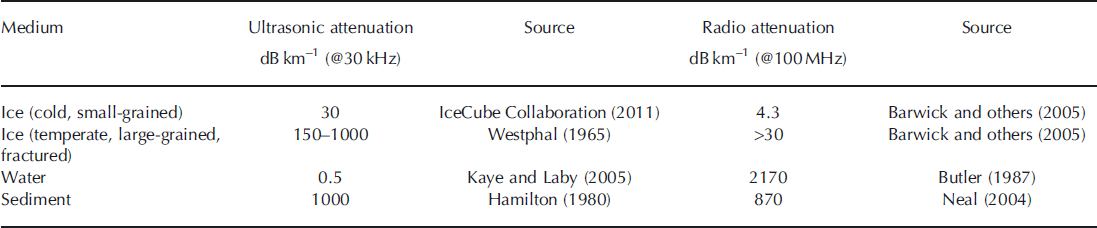
Table 2 gives insight into the scenarios of Figure 1. For transmission through ice alone (Fig. 1a), acoustic power decreases by 30 dB over 1 km, while radio signals are attenuated by only 4.3 dB over the same distance. All else being equal, then, radio is the preferred transmitter for communication through ice. However, when transmitting through ice and water (Fig. 1b) the situation is less clear, since the attenuation of radio waves in water is high (2170dB km–1).
3.2. Comparison of acoustic and radio attenuation
Figure 7a and b show the attenuation for both acoustic and radio signals, respectively, as contours of ice thickness and water depth. An attenuation of –60 dB (leftmost contour) means that a 1 W transmitter leads to a received power of 1 mW, which is well above the noise (see below), whereas the –120 dB contour (rightmost or uppermost) would give a received power of 1 pW, which is closer to the noise floor and therefore close to the range limit of the transmitter. The figure indicates that radio is unable to communicate through sufficient water depths to transmit from within subglacial lakes (which can be hundreds of metres deep) without a multi-sensor relay. Acoustic communications, in contrast, are limited by ice thickness. The water depth and ice thickness are shown for Subglacial Lake Whillans, Siple Coast, West Antarctica; Subglacial Lake Ellsworth, Pine Island Glacier catchment headwaters, West Antarctica; and Subglacial Lake Vostok, Vostok Station, East Antarctica. These three lakes are targeted for first-time entry within the next 3 years, and hence are illustrative of conditions where probes might be deployed. In all cases, we assume the wireless sensor is located at the base of the water column in the lakes. Either acoustics or RF might be suitable for wireless data transmission from Subglacial Lake Whillans (ice thickness 700 m, water depth ∼10 m) to the ice surface, whereas neither technology is sufficient to provide a full communications link from the other two subglacial lakes. However, Figure 7 does suggest the value of a dual system, where data are transmitted acoustically from the lake bed to a relay transmitter embedded within the ice sheet, at a distance of up to 1 km above the lake surface. The relay station then communicates via RF or cable with a receiving station on the ice surface.

Fig. 7. Comparison of attenuation levels of acoustic and radio communications from a wet subglacial environment. (a) Contours of acoustic attenuation for given water depth and ice thickness; (b) the same information for radio attenuation. The contours shown are for losses of 60, 90 and 120 dB: for a 1 W transmitter, these correspond to received signals of 1 μW, 1 nW and 1 pW respectively. Taking the 120 dB contour as a proxy for the limiting range of communication (i.e. the regions above and to the right of the 120 dB contour are out of range), acoustic attenuation is largely limited by the ice thickness, while radio attenuation is limited by water depth and becomes unfeasible through more than ∼50 m of water.
The communication scenarios described in Figure 7 do not account for the presence of sediment in the signal path. This may be applicable for a sensor resting on the bed of a subglacial lake, but not for communications from the lake sediments themselves or from the basal till layer of an ice stream (scenarios 3 and 4 in Section 1). Table 2 indicates that the presence of sediment in the signal path will have significant attenuative effects, and that these effects will be similar for both acoustic and RF communications. Figure 7 also does not account for any additional attenuative effect of ice fracturing, which might be present in the faster-flowing Whillans Ice Stream which overlies Sub-glacial Lake Whillans.
4. Non-Attenuation Losses in the Transmission Path
4.1. Transducer and coupling losses
Energy losses at the transducer depend upon the design of the acoustic transducer, and upon the efficiency of coupling to the surrounding medium. Typical commercial sonar transducers (e.g. Neptune Sonar T235) offer efficiencies of 50% when transmitting into water, i.e. half the electrical power input is converted into acoustic energy in the water. This 50% efficiency is equivalent to a 3 dB power loss from combined transducer and coupling losses.
4.2. Path loss
Path loss covers the energy lost due to beam spreading. For an isotropic source, from Huygens’ principle, the signal power intensity at any given radius is
where I is measured in W m–2 and P is the input power (Reference Kinsler, Frey, Cooppens and SandersKinsler and others, 1982).
It may be possible to reduce the path loss with a directional source, perhaps by up to 3 dB (Reference Kinsler, Frey, Cooppens and SandersKinsler and others, 1982). However, this would require the probe to be oriented correctly, which might be achieved in water by adjusting the internal mass distribution but is unlikely to be reliable in other media. In the rest of this work, therefore, the source is assumed to have an isotropic radiation pattern. Path loss is therefore a geometric effect, independent of transmission medium. Table 3 gives examples of power intensity, and path loss measured in decibels (relative to the received power at 1 m), as a function of distance from a 1 W source at r=0.
Table 3. Path loss values

4.3. Signal reflection
In pressurized (e.g. water-full) subglacial environments water directly contacts the ice. We assume a vertical signal path and a perpendicular ice/water interface (i.e. normal signal incidence). The intensity transmission coefficient Tat such an interface is given by

where r is the characteristic acoustic impedance, r=pc (Reference Kinsler, Frey, Cooppens and SandersKinsler and others, 1982). For pure water, r w=1.45x 10⁶kgm–2s–1 while for ice r i = 2.94 x 10⁶kgm–2s–1 (Reference Kaye and LabyKaye and Laby, 1995). Thus the intensity transmission coefficient T= 0.885, or equivalently ∼8 8% of the signal power is transmitted through the interface, a loss of ∼1 dB. If the surface is rough, scattering losses will lead to a lower transmission coefficient. For ice/air and water/air interfaces the transmission coefficients (calculated from Eqn (6)) are around T= 0.001, so any large air gaps in the transmission path (e.g. crevasses in ice near the surface) will reduce the signal by ∼30 dB at each interface. This is comparable to the path loss from increasing the range by a factor of 30 (see Table 3); large air gaps in the path cause sufficient attenuation to prohibit communications. It is worth noting that the empirical attenuation measurements listed above will include the effects of some interfacial reflections.
4.4. Noise
The coupling losses, path loss, reflections and attenuation control the signal strength at the receiver. In addition, this signal needs to be observable above background noise. Below the firn (and at the South Pole) absolute RMS noise values, integrated over the range 10-50 kHz, are less than p= 10mPa (Karg and others, 2009). Since acoustic intensity I = p2/pc, this corresponds to a noise level of 3.3 x 10⁻¹¹ Wm–2. Since the power consumption of the probe will determine its life-span, the surface receiver should be designed for maximum sensitivity. The receiver should therefore be deployed below the firn to minimize noise. We use a threshold for detection of 33 pW obtained in the following link budget calculations and note that the calculations could easily be repeated from other values.
5. Discussion
5.1. Link budget results and predicted communication range
One possible deployment scenario for a sub-ice-sheet probe might be to the base of a 2 m sediment layer in a 100 m deep subglacial lake, where ice thicknesses are ∼1 km. This is comparable to Subglacial Lake Whillans, although water depths here are of the order of tens of metres (Reference Fricker, Scambos, Bindschadler and PadmanFricker and others, 2007). Figure 8 shows the power requirements for communication in this scenario as a function of total ice-sheet thickness. This figure is derived from Eqn (1) using the various components stated or derived above. We assume a 30 kHz transmission frequency, as this is the centre point of the noise estimate given above. With a transmit power of 1 W, we can expect to receive unaveraged signals through 1 km of ice. Above 2 km of ice, power requirements can be considered prohibitive, since the required transmission power is several kilowatts.

Fig. 8. Power requirements for acoustic transmission through 2 m subglacial sediment, 100 m subglacial lake depth, and varying thickness of ice. 1W allows transmission through 1km of ice.
The link budget presented above suggests that acoustic techniques may be a useful means of retrieving data wirelessly from beneath the Earth’s ice sheets. The model contains various uncertain parameters, so it is helpful to conduct a sensitivity analysis to understand how these uncertainties affect our conclusions. Figure 9a shows the sensitivity of the link budget to variations in ice attenuation length (120, 150 and 180 m, i.e. attenuations of - 3 6 , - 2 9 and -24 dB km–1 respectively), noting that the attenuation quoted in IceCube Collaboration (2011) is given to an accuracy of ±20%. Within this range of ice attenuation, the transmission distance feasible with a 1 W source is still in the range 1-2 km. Figure 9b shows the effects of varying the lake depth (20, 100 and 500 m): we see that for small ice thicknesses, varying the lake depth changes the path length significantly, and hence the power requirements, whereas at large ice thicknesses the lake depth is less significant since the fractional change in path length is much lower. Figure 9c shows the effect of changing the transmitter efficiency (0.1, 0.5 and 1.0): since this is just a multiplier in the link budget, the effect is to move the entire graph up or down the vertical axis. Note that varying the reflection coefficient or receiver noise level would have similar effects. Figure 9d shows the effects of varying the sediment depth in which the probe is buried (0, 2 and 10 m). Overall, a general rule of thumb seems to hold: 1 W will allow communication through 1 km of ice.

Fig. 9. Sensitivity of acoustic power requirements to changes in ice attenuation length (top left), water depth (top right), transmitter efficiency (bottom left) and sediment thickness (bottom right).
5.2. System design and further work
Further data are needed on how noise levels in ice sheets might vary with geographic location and distance from the bed and the surface. Clearly some environments (i.e. those with flowing water close to the ice) might be significantly noisier than the South Pole. However, the noise bandwidth used for the discussion above is large (40 kHz), so the noise estimates are already somewhat conservative.
In cases where the limiting factor is the available transmitted power, averaging over n repeated signals improves the SNR by a factor of
![]() However, the subglacial probes discussed in this paper are likely to be limited by available energy (i.e. lifetime), so where possible it is more efficient to increase the transmission power than to repeat the transmission. For example, doubling the transmitted power increases the SNR by a factor of two, whereas transmitting a signal twice, and averaging, only increases the SNR by
However, the subglacial probes discussed in this paper are likely to be limited by available energy (i.e. lifetime), so where possible it is more efficient to increase the transmission power than to repeat the transmission. For example, doubling the transmitted power increases the SNR by a factor of two, whereas transmitting a signal twice, and averaging, only increases the SNR by
![]() although the total energy use is the same.
although the total energy use is the same.
The frequency chosen for communication will affect both the achievable data rate and the received signal strength. This work focuses on acoustic transmission frequencies around 30 kHz. It is useful to consider what limits there might be on the transmission frequency. Data rate requirements determine the minimum transmission frequency. The data rate required is determined by the number of sensors, the sampling sensitivity and the sampling rate. A typical specification might have five sensors, sampled with 12-bit analogue-to-digital conversion, once per minute, for a data requirement of 1 bits-1. Including a time stamp, identifying signature and data frame might raise this to 2 bitss–1. We can therefore, by the Nyquist-Shannon theory, modulate these data onto a 4 Hz signal. Note that, at this frequency, transmission must be continuous, whereas at higher frequencies transmission can be limited to short bursts, which will save power (e.g. doubling the frequency halves the required transmission period for a fixed data rate, and thus halves the power requirements). At frequencies up to 30 kHz, IceCube Collaboration (2011) find no frequency dependence of sound attenuation in South Polar ice, but results from Reference PricePrice (2006) suggest that, above ∼40kHz, scattering will dominate over absorption, and attenuation then increases rapidly with frequency. We therefore propose that communication is feasible over the band 4Hz–40kHz, but that increasing frequency within this range leads to a lower communications duty cycle and hence is likely to increase efficiency. Other factors affecting the choice of communications frequency are noise measurements at the receiver, and the efficiency of the transmitter and receiver. Further research into acoustic attenuation and noise in natural ice would allow us to determine whether a common standard frequency for through-ice communications is feasible, or if local variations require the choice of frequency to be made on a case-by-case basis, dependent on local geography (e.g. ice temperature and the level of fracturing).
Assuming the SPATS-measured attenuation length of ∼150 m (attenuation of ∼30 dB km–1), the range over which communications are possible is useful but not sufficient for all studies of interest. For example, Subglacial Lake Vostok, a large and well-studied lake, is up to 800 m deep and located beneath 4 km of ice (Reference Siegert, Carter, Tabacco, Popov and BlankenshipSiegert and others, 2005). Figure 8 suggests that even a 1 MW acoustic transmitter would be insufficient to transmit data from the lake bed to the ice surface. However, a series of relayed transmitters could conceivably be used to enable bed-to-surface wireless data transmission. A sensor/transmitter would communicate from the ice-sheet bed or lake bed to several hundred metres into the ice. A second transmitter here could then relay the data to the surface. In the absence of shear in the ice, a buried tethered receiver may be sustainable, and could greatly reduce transmission distances. In fast-flowing ice, one possibility is to use combined communications, with an acoustic relay through water into the ice, and then an RF transmission through the (relatively dry) ice to the surface. However, any relay-based system brings its own complications, as intermediate stages must listen as well as transmit, which leads to increased energy consumption.
6. Conclusions
Acoustic communications may be a useful technique for through-ice communication in situations where there is too much water present to permit effective RF communications. We find that acoustic communication is feasible, although highly dependent on through-ice attenuation, which varies with ice conditions. Estimates and measurements of acoustic attenuation in ice vary from 1 dBm–1, experimentally measured in Greenland ice sheet surface ice, to 1 dB km-1, predicted theoretically and experimentally for deep South Polar ice. In situ experiments on South Polar ice (200-500 m deep) indicate an attenuation of ∼30dBkm–1, and the link budget presented in Section 3 uses this value to predict a feasible communication length of 1 km through ice. Furthermore, inhomogeneities in the ice can lead to large, non-monotonic variations in the received signal strength, and cracks in the ice lead to severe attenuation, so any practical receiver should be tethered well beneath the ice surface. This work demonstrates that acoustic communication may be a useful tool for data communication through combinations of ice and water. The next step is to build and operate a working through-ice communications link.


