Introduction
In order to understand the relation between climate change and sea-level change, it is important to know the mass balance of the Antarctic ice sheet. Reference RobinRobin (1966) first suggested using a satellite-radar altimeter for ice-sheet surveying. Since then, the Seasat (Reference MacArthurMacArthur, 1978) and Geosat (Reference MacArthur, Marth and WallMacArthur and others, 1987) satellites have flown in orbits that reached latitudes of ±72.2°, thereby covering a major part of the Greenland ice sheet and a peripheral part of Antarctica. The Seasat and Geosat missions yielded an extensive set of radar-altimetric data that can be used for continental ice-sheet research, such as mapping the surface elevation (Reference Brooks, Campbell, Ramseier, Stanley and ZwallyBrooks and others, 1978; Reference Zwally, Brenner, Major, Martin and BindschadlerZwally and others, 1983), measuring surface-elevation changes (Reference ZwallyZwally, 1989; Reference Bentley and SheehanBentley and Sheehan, 1990) and mapping ice margins and grounding lines (Reference Thomas, Martin and ZwallyThomas and others, 1983; Reference Partington, Cudlip, Melntyre and King-HelePartington and others, 1987; Reference Zwally, Brenner, Major, Martin and BindschadlerZwally and others, 1987).
Because the Geosat and Seasat radar altimeters were designed for operation over the flat, relatively smooth ocean where the shapes of the return signals (“wave forms”) depend only on surface-scattering, the returns over the sloping, irregular ice sheet have to be re-analyzed, or "retracked" Reference Martin, Zwally, Brenner and Bindscharller(Martin and others, 1983). NASA's Goddard Space Flight Center retracked all the Seasat and Geosat altimeter data over the Greenland and Antarctic ice sheets to an overall precision of about 1.6m Reference Zwally, Brenner, Major, Martin and Bindschadler(Zwally and others, 1990). Their retracking algorithm estimated the peak power and the half-power point of the leading edge of the wave forms over the Greenland and the Antarctic ice sheets by fitting them with a five- or nine-parameter smoothing function that depended only on the shape of the return. The half-power point was taken as the indicator of the mean surface, a procedure that effectively neglects the volume back-scattering and topography, so is better suited to "ocean-like" wave forms than to wave forms from the high, cold interior of ice sheets. Reference Ridley and PartingtonRidley and Partington (1988) showed that volume-scattering as well as surface-scattering affects the wave forms over Antarctica and that neglecting volume scattering can introduce an error in elevation of as much as 3 m, depending on the retracking method and the location. In this paper, we present a retracking model that considers the surface- and volume-scattering, and apply it to a test area over East Antarctica. The surface elevations, according to our model, are about] m higher than those calculated by the NASA model (Reference Zwally, Brenner, Major, Martin and BindschadlerZwally and others, 1990).
Theoretical Model
The satellite-radar altimeter emits a pulse of electromagnetic radiation that is scattered back by the uppermost part of the ice sheet. To convert the two-way pulse delay time to distance, we need a realistic physical model of the interaction of the pulse with the ice sheet, i.e. with its upper surface and with its uppermost layers.
Surface back-scattering model
Reference Moore and WilliamsMoore and Williams (1957) showed that the mean return wave forms can be described as a function of time by the convolution of two terms:
where p r(t) is the received power at the satellite, p t(t) is the transmitted pulse profile and p m(t) is a term involving the distribution of scatterers, their back-scattering properties, and the effect of the antenna gain.
Reference BrownBrown (1977) generated an analytical solution for the mean ocean return under the approximation that the transmitted pulse shape, the altimeter's antenna pattern and the range distribution of scatterers obey a Gaussian distribution. The average surface-return power as a function of time (i.e. the surface-return "wave form"),Ps(δ),given byReference BrownBrown (1977, equation (13)), is
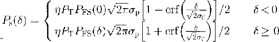
where ηis the pulse-compression ratio, PT is the peak transmitted power, σp=0.425τ,![]() and σ=t-2h/c. PFS is from Reference BrownBrown (1977), equation (9), modified to include the effect of the Earth's curvature (Rodriguez, 1988, equations (2), (3) and (4)).
and σ=t-2h/c. PFS is from Reference BrownBrown (1977), equation (9), modified to include the effect of the Earth's curvature (Rodriguez, 1988, equations (2), (3) and (4)).
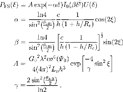
Here, PFS is the average impulse response from a smooth sphere, I0 is the zero-order Bessel function, of the second kind, δ is the reduced time, U(δ) represents the unit step function, t is time after emission of the pulse, h is the satellite height, Re is the radius of the Earth, c is the speed of light in vacuo, σp is the effective pulse resolution (based on the assumption of a Gaussian pulse shape), 7 is the altimeter's transmitted pulse width (3.125 ns),ξis antenna off-nadir angle, σs is the rms surface roughness,θ3dB is the angle at which the transmitted beam power is down by 3 dB, σ0(Ψ0) is the surface back-scattering cross section, Lp is the two-way free-space loss, G0 is the antenna bore-sight gain and λ is the radar wavelength. In this usage, σS is a measure of hath small-scale roughness and larger-scale surface topography; just how the effects are combined in σS cannot easily be ascertained.
Finally, we write
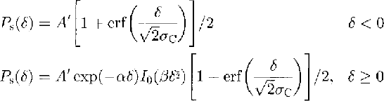
where![]() A' contains the quantities that do not vary in our study.
A' contains the quantities that do not vary in our study.
For a horizontal surface with a Gaussian distribution of scatterers, the mean surface height corresponds to the half-power point of the leading edge.
Volume back-scattering model
The average response [or a pulse back-scattered from within the fim, Pv(t), (assuming a horizontal, plane interface) has been given by Ridley and Partington (1988, equations (4) and (7)):
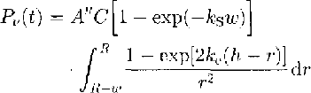
where R=h+v(t-(h/c)),v=2.35Ã-108 m s-l (the wave speed in the sub-surface layer) below the surface, and A"=2ΠPtT2G2λ2/(4Π)3.Pt. is the transmitted power, T is the surface-transmission coefficient, G is the gain of the transmitting antenna, A is the wavelength of the transmitted radiation, C is the Rayleigh phase function for back-scatter ![]() , kS is the scattering coefficient of firn, ω= vτis the pulse width and ke is the extinction coefficient in the firn. Since, to a very close approximation,
, kS is the scattering coefficient of firn, ω= vτis the pulse width and ke is the extinction coefficient in the firn. Since, to a very close approximation,

we can write

The depth of penetration d is defined by d = 1/ke for an extinction coefficient that is independent of the depth
Combined model
If we combine the surface- and volume-scattering models, we obtain
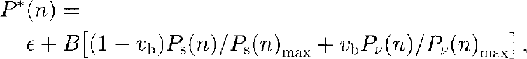
in which e is the noise level, Vb is the proportion of volume-scattering (0≤vb≤1),B is an amplitude coefficient (close to 1) adjusted to make P' (n) fit the normalized average wave form, n is the range-bin (gate) number, P'(n) is the modeled power that fits the normalized average wave form, Ps(n)max is the calculated maximum value of Ps(n), and Pv(n)max is the calculated maximum value of Pv(n). By taking the power ratios, we eliminate the effect of A′, A″ and the backscatter term C[l-exp(-kS w)].
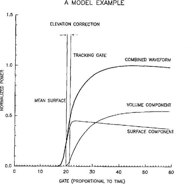
Figure 1 shows an example of a return-pulse shape according to the combined model. The mean surface is at the midpoint of the leading edge of the surface component and at the beginning of the volume component.

Fig. 1 An idealized radar-altimeter echo, showing the contributions of the surface and volume components. The “true” mean surface is defined by the mid-power point of the surface component, whereas the NASA-retracking defines the mean surface by the mid-power point of the combined wave form. The distance corresponding to the difference between the two is the elevation correction.
The primary assumptions of this model are:
-
(1) Volume-scattering above the mean surface is small and can be neglected.
-
(2) The scattering surface comprises a large number of random independent scattering elements that have a Gaussian distribution in heights.
-
(3) Scattering is a frequency-independent scalar process with no polarization effects.
-
(4) The firn has homogeneous scattering characteristics within the volume sampled by the altimeter.
-
(5) There is no multiple scattering.
-
(6) The ice grains are spherical.
In order to compare the model used in this paper with the model that only considers surface back-scattering, we define the elevation correction as the elevation calculated by the combined model minus the elevation calculated by the NASA model (Fig. 1)
Data Analysis
As a test of our method, we have applied it to several 1 month average Geosat wave forms over a small area of the ocean (55°-56° S, 80°–82° E). We found that the value of vb calculated by our program was sensitive to the mispointing angle on the order of a 0.1 change in vb for a 0.1° change in ξbut that vb could be reduced to only a few per cent by the proper choice of ξ(in the range of a few tenths of a degree). We interpret this as indicating a real mean mispointing angle and at the same time validating our procedure.
When our model is applied to returns from the interior ice sheet, the sensitivity to the pointing angle is much reduced, because of the large proportion of volume scattering. This is discussed further below.
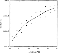
Our test area over the ice sheet lies in East Antarctica between 71.5° and 72° S and 80° and 90° E, divided into ten smaller blocks measuring 0.5° of latitude by 1° of longitude (Fig. 2). The surface height increases in the area from 2600 mat 80° E to 3100 mat 90° E (Fig. 3); the mean slope is slightly less than 0.2°. We used about 70000 wave forms from the Geosat Exact Repeat Mission collected between 9 November 1986 and 31 October 1987 for our test. The block-by-block average elevation profile for the whole area is shown in Figure 3.

Fig. 2 Map of part of East Antarctica showing the location of our test area (black rectangles). The map, with surface-elevation contours, is from Reference Zwally, Brenner, Major, Martin and BindschadlerZwally and others ( 1983). Latitudes and longitudes are in degrees south and east, respectively.

Fig. 3 Mean elevation in one-degree wide blocks across the test area (Fig. 2). Triangles are plotted at plus and minus one standard deviation.
To reduce the effect of the irregular shapes that arc characteristic of individual wave forms, averaging is necessary. There are two ways of averaging that we have considered. The first is to average a group of individual wave forms and then model the averaged wave forms. The averaged wave forms are easy to model but there is a difficulty in knowing how to align the wave forms correctly in the averaging process. The second way is to model the individual wave forms first, then average the model parameters. In this method, an elevation correction can be acquired for single points, but the effect of irregular topography on the individual wave forms makes model fitting difficult and the parameters less reliable. In this paper, the first method, which also consumes less computer time, was used.
Three wave-form-averaging methods were tried:(I)simple averaging of wave forms as they appeared in the gates without re-alignment,(2)aligning the wave forms at their “center of mass” as first described by Reference Wingsham, Rapley, Griffiths, Guyenne and HuntWingham and others (1986)and (3) aligning the wave forms at the midpoints of their first ramps (the NASA retracking; point).We found the smallest standard deviation in the power of the averaged wave forms for method (3),so we used that method in our analysis.
Because the average mispointing angle of the Geosat altimeter was 0.2° and the mean surface slope of the region concerned was also 0.2°, we have tested the combined effect by using different mispointing angles (0°,0.2°, 0.4°);the difference between the parameters calculated in the three cases was small- usually only a few per cent and always less than 10%. Because the effect is small and because, to a first approximation, mispointing angles that are less than the surface slope will have opposite effects, we have applied our analyses using ξ=0.2°, corresponding to the mean slope
The averaged wave forms vary with location and time. Figure 4 shows wave forms averaged monthly over a single 1° block and averaged for 1 month across the entire test region. We believe part of the variation shown is due to changing penetration. The density, temperature, grain-size and water content of the snow all affect the extinction coefficient and all can change with location and time.
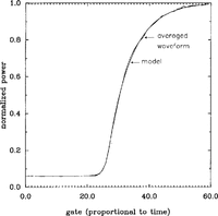
Our model fits the averaged wave forms very closely. An example is shown in Figure 5, wherein the smooth curve is from the model and the wiggly curve is the averaged wave form. We did not have difficulty fitting the data from 85° to 90° E as Reference Partington, Cudlip, Melntyre and King-HelePartington and others (1987) had. We do not know whether that is because of the differences in our models or differences in our averaged wave forms.

Fig. 4 Mean monthly wave forms for a single block (82°-830 E), for the months of November 1986 through October 1987. b. Mean July 1987 wave forms in one-degree-wide blocks for the ten blocks between 800 and 90° H.

Fig. 5 A sample of a mean wave form together with the fitted model curve.
Results And Discussion
From model fitting to the averaged wave forms, we have evaluated elevation corrections, extinction coefficients ke proportions of volume-scattering vb and surface roughnesses. To examine how these parameters vary with location and time, we have calculated mean values of each for the whole year within each 1° wide block (Fig. 6) and over the whole ten-block test region for each month (Fig. 7). We have plotted standard deviations in those figures; standard errors of the means would be smaller by a factor of about 3.3 (i.e. by √ n, where n is 12 (months) for Figure 6, and ten (blocks) for Figure 7).
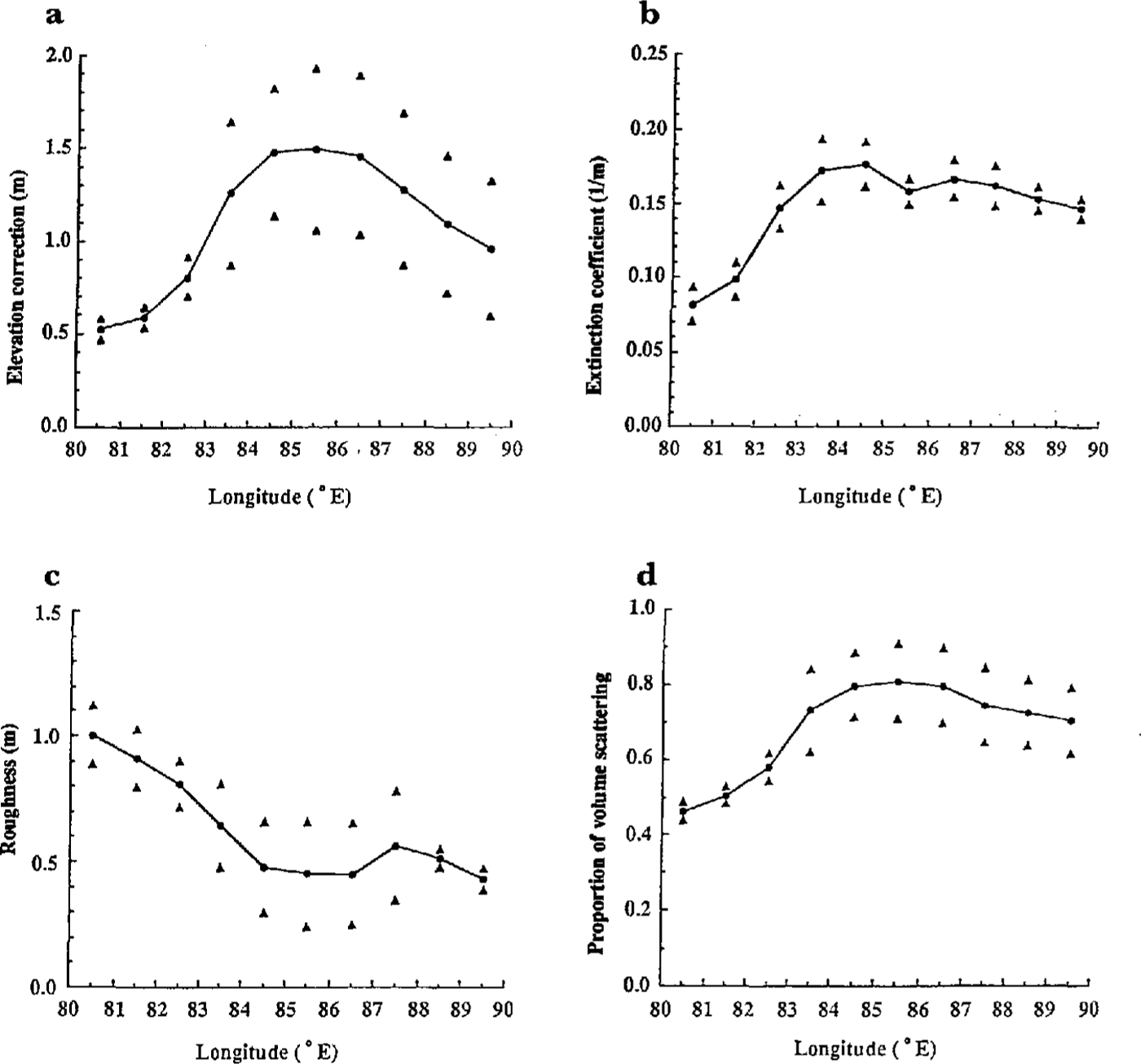
Fig. 6 Whole-year mean parameters in one-degree-wide blocks as a function of longitude. Triangles are plotted at Plus-and minus one standard deviation. a. Elevation corrections; b. Extinction coefficients (ke); c. Surface roughnesses; d. Fractions of volume-scattering, (vb).

Fig. 7 Whole-region mean monthly parameters as a function of time through one year (November 1986 through October 1987). Triangles are plotted at plus-and-minus one standard deviation. a. Elevation corrections; b. Extinction coefficients (ke); c. Surface roughnesses; d. Fractions of volume-scattering (vb).
Yearly averages show significant spatial variations (Fig. 6). The elevation correction, extinction coefficient and vb are all larger at the higher elevations in the eastern part of the test region, whereas the surface roughness decreases eastward. The first three parameters are strongly correlated. The maxima in vb and the elevation correction coincide, as do the minima. On the other hand, vb has its maximum when the depth of penetration is at a minimum. This is because, with deeper penetration, less volume-scattered signal arrives within the modeled part of the wave forms. The volume-scattering that most affects the measured elevation occurs at depths between 0 and 15 m. The extinction-coefficient values acquired here are similar to the value, 0.14m-1, measured by Reference Hofer and MatzlerHofer and Matzler (1980) on cold Alpine snow.
The seasonal changes in the mean monthly parameters (Fig. 7) are less significant than the spatial changes hut there still seem to be some real effects. In particular, the elevation correction appears to change by some tens of centimetres over the year; such a variability would be important in a search for real changes in surface elevation.
Future Work
At this point, our combined model includes the effects of the antenna pattern, the surface slope, and the Earth's curvature on the surface-scattered component of the return but not on the volume-scattered component. Although we believe the neglected effects are small, we plan to evaluate them further.
Our model has been applied only to a small test area. When we are fully satisfied with it, we will apply it over the whole East Antarctic region of our interest (80-140° E).
We hope to develop further application of the model to fit individual wave forms, so that it can be used as a retracker. Retracking in this way might be more precise than retracking based on a model of surface-scattering only.
Since, according to our analysis, the penetration depth is more than 12 m, sub-surface features might be detected in future studies
Conclusions
Penetration of the radar signal into the firn on the cold East Antarctic ice sheet causes an error, if the penetration is not taken into account, of the order of 1 m. The effect varies laterally, with changing surface elevation. Temperature and snow conditions also depend on surface elevation; we have no information on which parameters control the volume scattering. We have found small temporal variations that would affect measurements of the change in surface elevation with time.
Acknowledgements
This work was supported by NASA grant NAGW-1773. This is contribution No. 545 of the Geophysical and Polar Research Center, University of Wisconsin-Madison. We thank two anonymous referees for their helpful comments, which have led to substantial improvements in our paper.