


Introduction
Sea ice modifies the exchange of mass, energy and momentum in the planetary boundary layer, and therefore the local and regional climate as well as the general circulation of the atmosphere and the thermohaline oceanic circulation are influenced by sea-ice changes via complex feedbacks in the atmosphere-ocean-sea-ice system.
The seasonal variability of the sea-ice extent in the Arctic ranges from 15 × 106 km2 in March to 7.6 × 10⁶ km2 in September, showing extensive temporal and spatial variability. Data analyses show large inter- and intra-annual variabilities of the sea-ice extent (Reference Parkinson, Cavalieri, Gloersen, Zwally and ComisoParkinson and others, 1999). Based on consistent sea-ice concentration (SIC) time series (1979−96) from the Scanning Multichannel Microwave Radiometer (SMMR) and Special Sensor Microwave/Imager (SSM/I) passive-microwave radiometers, a continuous decrease of Arctic sea-ice cover of 2.9% ± 0.4% per decade can be found (Reference Cavalieri, Gloersen, Parkinson, Comiso and ZwallyCavalieri and others, 1997). The negative trend is largest during summer. It has strengthened since 1990 and is most pronounced in the East Siberian and Laptev Seas (Reference Serreze, Maslanik, Key, Kokaly and RobinsonSerreze and others, 1995; Reference Maslanik, Serreze and BarryMaslanik and others, 1996). A linear least-squares regression for May-August 1979−96 for the Laptev Sea ice area yields a negative trend of 66184 km2, i.e. a sea-ice area reduction of 36 768 km2 per decade (5.5% per decade) (Fig. 1).
Fig. 1. Time series of monthly anomalies for the Laptev Sea sea-ice area derived from SMMR and SSM/I data, May-October 1979−96. See Figure 2 for reference area. Note the breaks in the time series from October to May. The data for this plot were obtained by taking the monthly value for the individual month and subtracting the average value for that month over the 18 year period. The vertical bars mark the months May-August which were simulated with HIRHAM4; light/dark grey: positive/ negative sea-ice anomalies in the Laptev Sea.
Reference Walsh and JohnsonWalsh and Johnson (1979) and Reference Slonosky, Mysak and DeromeSlonosky and others (1997) find significant correlations between sea ice and the atmospheric circulation, based on data with a relatively coarse spatial and temporal resolution. In a simulation with a coupled ice-ocean model, Reference Proshutinsky and JohnsonProshutinsky and Johnson (1997) show, in agreement with observational data, that the Arctic Ocean’s circulation regime and sea-ice drift are primarily driven by the near-surface wind fields. Sea-ice anomalies in relatively small areas on time-scales of several days to weeks seem to be strongly coupled with cyclones (Reference Maslanik and BarryMaslanik and Barry, 1989; Reference Maslanik, Serreze and BarryMaslanik and others, 1996). The results of a high-resolution coupled regional climate model over the Arctic highlight the importance of regional atmospheric circulations in driving interannual variations in Arctic ice extent (Reference Maslanik, Lynch, Serreze and WuMaslanik and others, 2000). The focus in our paper is on the Laptev Sea ice variations and their relation to the atmospheric circulation.
Datasets
Four different datasets have been used in the study (see Table 1 for the dataset descriptions and Figure 2 for the locations of the data):
-
1. The sea-ice concentration data come from satellite observations of the SMMR and SSM/I passive microwave radiometers. They are derived from the brightness temperatures using the NASA-team algorithm with global tie points. Gaps in the SMMR data record (1 January 1979 to 20 August 1987) of every second day were closed by a linear interpolation between successive time-steps. The spatial coverage is reduced in relation to the original data as indicated in Figure 2. The sea-ice area anomaly time series is calculated without grid elements bordering on land pixels to exclude false sea-ice concentrations due to land-ocean spillover.
-
2. The daily mean sea-level pressures (SLPs) north of 50° N were obtained from the U.S. National Centers for Environmental Prediction/U.S. National Center for Atmospheric Research (NCEP/NCAR) re-analysis project (Reference KalnayKalnay and others, 1996).
-
3. Cyclone frequencies and intensities for the Laptev Sea area (70−85° N, 70−160° E) were extracted from the Arctic Cyclone Track Data Set, 1966−93, available from the U.S. National Snow and Ice Data Center (NSIDC) (Reference SerrezeSerreze, 1995).
-
4. The mesoscale atmospheric data were obtained through simulations of the regional climate model HIRHAM4, which is applied over the whole Arctic (Fig. 2, "HIR-HAM4 model domain") with a horizontal resolution of 0.5° in latitude and longitude corresponding to grid elements of about 50 km × 50 km and 19 vertical levels from ground up to 10 hPa. Simulations were performed in the summers (May-August) of four years (1983,1990,1991, 1995) with negative sea-ice anomalies and four years (1986, 1987, 1992, 1993) with positive sea-ice anomalies in the Laptev Sea. Several studies, such as Reference Dethloff, Rinke, Lehmann, Christensen, Botzet and MachenhauerDethloff and others (1996) and Reference Rinke, Dethloff, Spekat, Enke and ChristensenRinke and others (1999), show the performance of this atmospheric model over the Arctic which uses European Centre for Medium-range Weather Forecasts (ECMWF) analysis for the lower and lateral boundary forcing. The sea-surface temperature (SST) at the lower boundary is updated daily by ECMWF analysis. Sea ice covers an entire gridbox with a 2 m thickness when the SST is below −1.8°C For the present study, time series of SLP and 10 m wind speed for two years with negative and positive sea-ice area anomalies were extracted at a reference point (76.4° N, 125.8° E) in the Laptev Sea (Fig. 2).
Table 1. Datasets used in this study
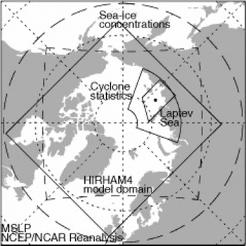
Fig. 2. Spatial distribution of the datasets. the dot symbol marks the reference point at approximately 76.4° N, 125.8° E, used for the laptev sea time series. dashed line at 50° N: NCEP/NCAR re-analysis data; dashed box: HIRHAM4 model domain; solid box: NSIDC sea-ice concentrations; solid semicircle: reference area for cyclone statistics.
Relationship between Large-Scale Circulation and Sea-Ice Concentrations
First, an empirical orthogonal function (EOF) analysis was applied to datasets 1 and 2, i.e. the anomalies of monthly mean SIC and SLPs, to extract the dominant spatial patterns and their temporal variability and strength. The relationship between these two datasets is examined with a canonical correlation analysis (CCA) based on the Reference Barnett and PreisendorferBarnett and Preisendorfer (1987) method. Input data for the CCA are the calculated EOFs whereby 8 SIC and 11 SLP EOFs were taken into account. The CCA finds a set of mutually uncorrelated canonical correlation patterns (CCPs) whose coefficients share a maximum correlation and indicate the temporal evolution and strength of the pattern.
Table 2 summarizes the results of the CCA. The first correlated mode of variation (the estimated canonical correlation is 0.84) represents about 53% and 40% of the total variability of the monthly mean SIC and SLP, respectively. The pattern of the SLP shows the polar vortex and the mass see-saw between the central Arctic and mid-latitudes, the so-called Arctic Oscillation (Reference Thompson and WallaceThompson and Wallace, 1998). The pattern of the SIC shows the seasonal decrease of SIC in the Arctic’s marginal seas, while the second correlated mode (the estimated canonical correlation is 0.7) shows a rather rare atmospheric circulation pattern (a small global variance of only about 3%). The latter suggests that cyclone activity can be a driving mechanism of the SIC anomalies (not shown).
Table 2. Summary of the CCA between 11 SLP and 8 sic dominant spatial patterns
The CCP pairs 3 and 4 seem to be important to explain the sea-ice anomalies in the Laptev Sea (the estimated canonical correlation is about 0.3 in each case). In CCP 3, an atmospheric pattern with 15.3% of explained global variance is coupled with a rather rare sea-ice pattern (Fig. 3). Parts of the northern and central Laptev Sea, the eastern Kara and Barents Seas account for the SIC global variance of only 2.1%, but local variances in these areas (not shown) are as high as 30%. A positive coefficient of the SLP pattern which corresponds to an anticyclonic circulation regime prevails especially in the period 1984−88. The SIC decreases at the same time. This is in accordance with the findings of, for example, Reference Proshutinsky and JohnsonProshutinsky and Johnson (1997) that during these regimes the Transpolar Drift Stream shifts towards the Eurasian Shelf seas, which might enhance sea-ice export out of the Siberian marginal seas.

Fig. 3. Third pair of CCPS of (a) sea-level pressure eofs (hpa) and (c) sea-ice concentration eofs (%). (b, d) time series of the corresponding canonical correlation coefficients, normals to variance 1. light/dark grey horizontal bars mark anticyclonic/cyclonic circulation regimes (Reference Polyakov, Proshutinsky and Johnsonpolyakov and others, 1999). note the breaks in the time series from august to may. base data: datasets 1 and 2.
Similar conditions are evident in CCP pair 4 (Fig. 4). Up to 10% of the local variance is explained by the SIC pattern east of the Taymyr peninsula, in areas which are part of the Taymyr ice massif In 1983, 1990 and 1995, years with strong negative SIC anomalies in the Laptev Sea, the canonical coefficients are negative, meaning a SIC decrease in these areas. The cyclonic circulation in the northern parts can lead to an increased ice import, but, on the other hand, should increase zonal transport north of 75° N and enhance warm-air advection. The coefficient of the SIC pattern remains positive most of the time during the anticyclonic regime in 1979 and 1984−88.

Fig. 4. As in figure 3 but relative to the fourth pair of CCPS and corresponding canonical correlation coefficients.
Summarizing, there is evidence that positive and negative sea-ice anomalies may originate from modifications of the sea-ice cover, especially in the central and northern parts of the Laptev Sea and the Taymyr ice massif. They are linked to atmospheric circulation patterns in the central Arctic as shown by CCPs 3 and 4. These findings are similar to those of Reference Deser, Walsh and TimlinDeser and others (2000), who conclude that summer sea-ice variations appear to be initiated by atmospheric anomalies over the high Arctic in late spring.
Influence of Synoptic Activity on Sea-Ice Concentration
In order to investigate the relationship between the sea-ice variations and the synoptic activity, we have chosen a twofold approach: First, the frequency and intensity of polar cyclones over the Laptev Sea (dataset 3) is compared with the anomalies of the total Laptev Sea sea-ice concentrations. Secondly, time series of local meteorological variables in the planetary boundary layer from the HIRHAM4 model simulations (dataset 4) are compared to the sea-ice concentrations at approximately the same positions in the datasets.
From May to August 1979−93 a total number of 1590 closed low-pressure systems is registered in the Laptev Sea area, 15.4% of which were cyclogenesis and 13.7% cyclolysis events. The average is 26.5 systems per month. The number of systems increases by 2.27 per season (May-August), while the mean central pressure decreases slightly. An increased cyclone activity can enhance warm-air advection and lead to a larger shear stress and sea-ice drift. Baroclinic instabilities can arise which in turn lead to an increased ice divergence (Reference Tansley and JamesTansley and James, 1999). This is what happened in May 1990, when a strong low-pressure system was located northwest of the Laptev Sea (Reference Serreze, Maslanik, Key, Kokaly and RobinsonSerreze and others, 1995).
We correlated sea-ice area anomalies and cyclone activity (numbers of low-pressure systems, mean central pressure as cyclone intensity, numbers of cyclones with pressure below 990 hPa) in the Laptev Sea, but a simple relationship between these parameters does not exist (Fig. 5). Both positive and negative ice anomaly years ― independent of the atmospheric circulation regime ― show a large cyclone activity (eg. 1986,1990).

Fig. 5. Time series, may-august 1979−93, of monthly means of (a) laptev sea ice area anomalies, (b) cyclone counts at 70−85° N, 70−160° E, (c) mean central pressure of these systems, and (d) the number of systems with a central pressure of <990 hpa.
In the next step we correlated Laptev Sea SIC data with meteorological parameters extracted from the high-resolution atmospheric model simulations. The time series for 1986 and 1990, plotted in Figure 6, are examples of years with positive and negative sea-ice anomalies in the central Laptev Sea at approximately 76.4° N, 125.8° E.
Fig. 6. Tine series of (a) sea-ice concentrations (NSIDC), (b) sea-level pressure and (c) 10 m wind speed (HIRHAM4) at approximately 76.4° N, 125.8° E, and (d) cyclone counts (arctic cyclone track data set) at 70−82° N, 90−145° E, for summers with positive (1986) and negative (1990) sea-ice area anomalies in the laptev sea. the temporal resolution of SLP is 6 hours. the 10m wind-speed components are averaged over 6 hours and low −pass filtered (with a filter width of 5 elements). the SIC and the number of all registered, closed cyclones between 70−82° N and 90−145° E have a temporal resolution of 1 day.
From May to July 1986, the SIC at the reference point remains above 80% with few exceptions. The measured SIC reduction around 5 June is probably caused by melt ponding. With no free drift conditions the cyclone activity in June is unlikely to have an immediate effect on the SIC. The SIC decrease at 8 August is accompanied by a pressure decrease to about 998 hPa and wind speeds of about 20 m s −1. After the slightly enhanced synoptic activity in mid-July and an increase in the system’s intensity (second spatial derivation, not shown), the SIC starts to drop by around 40% during the last 3 days in August and reaches open-water conditions 9 days later in early September.
During May 1990 the SIC is constantly above 90%. Cyclone activity is as high as 35 systems per month, with central pressures at a minimum of 976 hPa. Each time wind speed exceeds 20 ms−1, there follows a slight decrease in SIC. The reduced SIC in the first half of June is probably caused by melt ponding and a substantial meltwater buildup within and at the base of the snow cover (Reference Bareiss, Eicken, Helbig and MartinBareiss and others 1999). Cyclone activity decreases to 12 systems, and wind speed drops to a minimum of 1.6 m s−1. In the second half of June, SIC starts to decrease continuously until open water is reached, with a sharp decrease at the end of the month of approximately 10% SIC in 24 hours. This is not accompanied by anomalously intense atmospheric conditions. The spatial distribution of the SIC data shows that the West New Siberian polynya extends to this position. A distinction between dynamic and thermodynamic components is currently not possible.
The data suggest that atmospheric processes, especially Arctic cyclones, may predispose the ice cover by enhancing the shear stress on the sea ice, which facilitates ablation and drifting at a later stage. Reference Maslanik, Lynch, Serreze and WuMaslanik and others (2000) showed in a coupled model experiment for 1990 the importance of regional atmospheric circulation placement and strength of high- and low-pressure systems in driving patterns and velocity of sea-ice transport.
Summary
The influence of the atmospheric circulation on the SIC at different spatial and temporal resolutions has been investigated for May-August 1979−96 for the Laptev Sea. The major conclusions are the following:
-
1. The CCA shows SIC patterns statistically significantly correlated to large-scale SLP fields. The SIC anomalies in the Laptev Sea depend on relatively rare atmospheric circulation patterns which might be attributed to cyclone activity. Negative SIC anomalies in the central, northern and northwestern parts (Taymyr ice massif) seem to depend on ice drift caused either by a shift of the large-scale ocean currents or by wind-driven ice export, when cyclonic circulation dominates the northern Laptev Sea.
-
2. Short-term SIC variations seem to be connected to synoptic-scale low-pressure systems, but no simple relationship can be found between the SIC decrease and cyclone activity
A complex time-dependent combination of dynamic and thermodynamic processes, including sea-ice properties such as ice thickness and sea-ice drift to and from adjacent areas, must be taken into account. Further diagnostic studies of single events incorporating drift data and experiments with a coupled regional-scale model as started by Reference Maslanik, Lynch, Serreze and WuMaslanik and others (2000) are necessary.
Acknowledgements
We would like to thank: EOSDIS NSIDC Distributed Data Archive Center, University of Boulder, Colorado, for providing the SIC data record and the Arctic Cyclone Track Data Set; NCEP/NCAR for re-analysis data via U.S. National Oceanic and Atmospheric Administration Climate Diagnostics Center; Deutsches Klimarechenzentrum and Max Planck Institute for Meteorology Hamburg, for providing computational resources and software. The comments of two anonymous reviewers aided in the preparation of this paper.


