


Introduction
Driven by rising atmospheric temperatures, the Greenland ice sheet (GrIS) is losing mass at an accelerated rate (van den Broeke and others, Reference van den Broeke2009; Shepherd and others, Reference Shepherd2012; Hanna and others, Reference Hanna2013; van Angelen and others, Reference van Angelen, van den Broeke, Wouters and Lenaerts2014; Kjeldsen and others, Reference Kjeldsen2015; Bevis and others, Reference Bevis2019). The total mass loss of the GrIS over the 2010–18 period is estimated to be 286 ± 20 Gt a−1, with 49 ± 3 Gt a−1, coming from Southeast Greenland (Mouginot and others, Reference Mouginot, Rignot, Bjørk, Broeke, Millan, Morlighem, Noël, Scheuchl and Wood2019). In the remainder of the 21st century, it is expected that increased meltwater runoff, and the associated decrease in surface mass balance (SMB) will dominate solid ice discharge as the GrIS's largest contribution to sea level rise (e.g. Enderlin and others, Reference Enderlin2014). SMB is defined as snow accumulation and wind-driven snow redistribution (through erosion or redeposition), minus runoff, where accumulation is the difference between snowfall and evaporation/sublimation (Lenaerts and others, Reference Lenaerts, Medley, van den Broeke and Wouters2019). In this study, we ignore redistribution, as it is two orders of magnitude smaller than snowfall integrated across Southeast Greenland (Lenaerts and others, Reference Lenaerts, van den Broeke, van Angelen, van Meijgaard and Déry2012). Although it is not the focus of this study, redistribution likely explains a large portion of the small scale (<1 km) variability in accumulation (Dattler and others, Reference Dattler, Lenaerts and Medley2019). Additionally, there is little-to-no-runoff expected in the period we observed between the last peak melt and mid-spring. Therefore, we assume SMB to be equal to accumulation in this study.
Southeast Greenland, which we define as the region between 45° W to 33° W and 60° N to 67° N (Fig. 1), encompasses the area with the highest accumulation rates on the GrIS (Berdahl and others, Reference Berdahl2018; Shepherd and others, Reference Shepherd2019). Regional climate models (RCMs) suggest that Southeast GrIS receives ~30% of the total GrIS snowfall (Miège and others, Reference Miège2013). Therefore, interannual variations in this region strongly influence the total GrIS mass balance, even determining the sign of the total mass balance during some years (Burgess and others, Reference Burgess2010). However, evaluating the rate and pattern of accumulation in climate models is challenging, as there are very few in situ observations available on the Southeast GrIS (e.g. Ettema and others, Reference Ettema2009; Hanna and others, Reference Hanna2011; Lucas-Picher and others, Reference Lucas-Picher2012; van den Broeke and others, Reference van den Broeke2016; Fettweis and others, Reference Fettweis2017; Montgomery and others, Reference Montgomery, Koenig and Alexander2018).
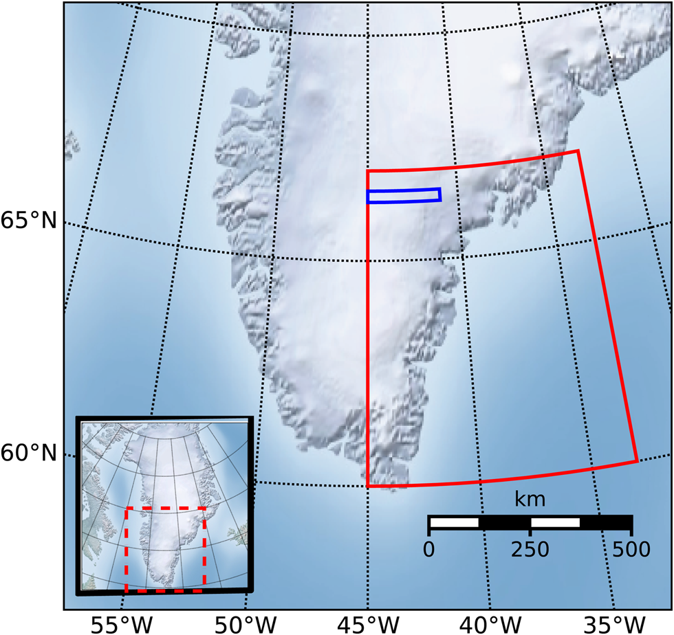
Fig. 1. Overview of our bounded study region in Southeast Greenland (red) and flight-line case study region (blue). Inlaid box is a map of Greenland with a box around the zoomed area (dashed red).
Using airborne observations, we can address the lack of in situ accumulation observations in Southeast Greenland. A first compilation of GrIS accumulation rates derived from NASA Operation IceBridge (OIB) airborne snow radar was presented by Koenig and others (Reference Koenig2016) for the period of 2009–12. Here, we extend the time series of radar-derived accumulation rates to 2017 focusing on Southeast Greenland, using observationally constrained, gridded firn density products to convert radar-derived depth to accumulation. In addition, we compare these radar-derived accumulations with two RCMs, the Modèle Atmosphérique Régional version 3.9 (MAR) and the Regional Atmospheric Climate Model version 2.3p2 (RACMO2). The goal of this work is to understand the magnitude, spatiotemporal variability and uncertainty of radar-derived accumulation in Southeast Greenland, and to provide an initial assessment of RCM performance in simulating Southeast Greenland SMB.
Observations, instruments and models
Operation IceBridge airborne snow radar data
From 2009 to 2019, the Center for Remote Sensing of Ice Sheets (CReSIS) at the University of Kansas operated the snow radar onboard the NASA P3-B and DC8 aircraft during OIB missions. We use the radar data from 2009 to 2017 due to data and model output availability at the time of the study. This radar maps internal annual accumulation layers ranging from 10 cm to >1 m (Panzer and others, Reference Panzer2013). These data, IceBridge snow radar L1B Geolocated Radar Echo Strength Profiles, Version 2, are available from the National Snow and Ice Data Center (NSIDC; Paden and others, Reference Paden, Leuschen, Rodriguez-Morales and Hale2014). The snow radar detects isochronal layers in the firn and are dated by assuming annual stratigraphy and counting each layer down from the surface (Medley and others, Reference Medley2013; Koenig and others, Reference Koenig2016). Annual layering of accumulation can be detected because radar reflection horizons represent contrasts in the material's dielectric permittivity, attributed to isochronous buried sequences, ice crusts and snow layers (Medley and others, Reference Medley2013). The radar uses a frequency-modulated continuous wave architecture that operates in the 2–6.5 GHz frequency range with a vertical resolution of ~5 cm (Medley and others, Reference Medley2013; Panzer and others, Reference Panzer2013). We chose this radar over the other radars aboard OIB because of its high vertical resolution and shallower penetration depth that allow the radar to measure recent accumulation rates (past ~1 to 20 years).
In-situ density observations
The SUMup (SUrface Mass balance and snow depth on sea ice working group) dataset provides snow and firn density profiles and accumulation measurements across the entire GrIS (Montgomery and others, Reference Montgomery, Koenig and Alexander2018). Density profiles from 306 locations on the GrIS are used to compare modeled with observed densities in the top meter of firn (Figs 2a and b; Renaud, Reference Renaud1959; Ohmura, Reference Ohmura1991, Reference Ohmura1992; Alley, Reference Alley1999; Bolzan and Strobel, Reference Bolzan and Strobel1999a, Reference Bolzan and Strobel1999b, Reference Bolzan and Strobel1999c, Reference Bolzan and Strobel1999d, Reference Bolzan and Strobel1999e, Reference Bolzan and Strobel1999f, Reference Bolzan and Strobel1999g, Reference Bolzan and Strobel2001a, Reference Bolzan and Strobel2001b; Miller and Schwager, Reference Miller and Schwager2000a, Reference Miller and Schwager2000b; Wilhelms, Reference Wilhelms2000a, Reference Wilhelms2000b, Reference Wilhelms2000c, Reference Wilhelms2000d; Bales and others, Reference Bales, McConnell, Mosley-Thompson and Csatho2001; Mosley-Thompson and others, Reference Mosley-Thompson2001; Conway, Reference Conway2003; Dibb and Fahnestock, Reference Dibb and Fahnestock2004; Dibb and others, Reference Dibb, Whitlow and Arsenault2007; Mayewski and Whitlow, Reference Mayewski and Whitlow2009a, Reference Mayewski and Whitlow2009b, Reference Mayewski and Whitlow2009c, Reference Mayewski and Whitlow2009d; Harper and others, Reference Harper, Humphrey, Pfeffer, Brown and Fettweis2012; Benson, Reference Benson2013, Reference Benson2017; Miège and others, Reference Miège2013; Hawley and others, Reference Hawley2014; Koenig and others, Reference Koenig, Miège, Forster and Brucker2014; Baker, Reference Baker2016; Chellman, Reference Chellman2016; Machguth and others, Reference Machguth2016; Schaller and others, Reference Schaller2016, Reference Schaller, Kipfstuhl, Steen-Larsen, Freitag and Eisen2017; Cooper and others, Reference Cooper and Cooper2018; MacFerrin and others, Reference MacFerrin2018a, Reference MacFerrin, Stevens, Abdalati and Waddington2018b). We use 35 density profiles from Southeast Greenland to compare with RCM density in the top 5 m. Most density profiles were retrieved from firn cores (98%) with average core depths >10 m while a small fractions were taken from snow pits (2%) with depths <2 m.
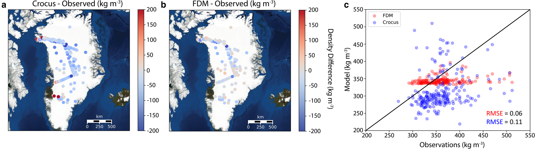
Fig. 2. Difference of average density (kg m−3) in the top meter between (a) Crocus or (b) FDM and SUMup observations across Greenland. (c) Scatterplot of Crocus and FDM densities vs observations.
MAR and RACMO2 simulated SMB
We use our radar-derived observations to evaluate the accumulation simulated by two RCMs (MAR and RACMO2) over Southeast Greenland. MAR and RACMO2 are forced at their lateral boundaries by a reanalysis dataset (ERA-Interim 1979–2018) (Noël and others, Reference Noël2016; Fettweis and others, Reference Fettweis2017; Delhasse and others, Reference Delhasse, Fettweis, Kittel, Amory and Agosta2018). Monthly gridded SMB from MAR (originally 15 km) and RACMO2 (originally 5.5 km) is downscaled to a 1-km spatial resolution, and provide the atmospheric input used to derive density profiles (see ‘Crocus and FDM modeled density' section). The RCM SMB products used here are downscaled based on the local regression to elevation from higher resolution digital elevation models (Noël and others, Reference Noël2016; personal communication from Fettweis, 2019). These downscaled accumulation model products are used to compare with our radar-derived accumulation. Previous studies have shown that both MAR and RACMO2 SMB products compare well with available in situ observations on the GrIS (Fettweis and others, Reference Fettweis2017; Noël and others, Reference Noël2018), although an evaluation of Southeast GrIS has so far been hampered by the paucity of observations in that region.
Crocus and FDM modeled density
Spatially gridded density profiles are taken from two firn models, Crocus and the Firn Densification Model of the Institute for Marine and Atmospheric research Utrecht (IMAU-FDM v2.3p2) (referred to hereafter as Crocus and FDM, respectively). Crocus model output, available at a horizontal resolution of 15 km, is forced with atmospheric data and mass fluxes from MAR (Fettweis and others, Reference Fettweis2017). Crocus is a snow model that simulates energy and mass evolution of a snow cover at a given location and provides vertical density profiles (Brun and others, Reference Brun, Martin, Simon, Gendre and Coléou1989, Reference Brun, David, Sudul and Brunot1992). The FDM model output, available at a 5.5 km spatial and 10-daily (instantaneous) temporal resolution, is a time-dependent, 1-D model that keeps track of the density and temperature in a vertical firn column, and is driven by atmospheric input originating from another RCM, RACMO2 (Kuipers Munneke and others, Reference Kuipers Munneke2015; Ligtenberg and others, Reference Ligtenberg, Kuipers Munneke, Noël and van den Broeke2018). Model output prior to our study period is used to understand density differences across the GrIS since the majority of observations from SUMup are not from 2009 to 2017 (Fig. 2). Both densification models can simulate liquid water content, percolation, layer saturation and refreezing in firn. The FDM can store liquid water through capillary forces, which best simulates the processes occurring in the percolation zone in Southeast Greenland (Ligtenberg and others, Reference Ligtenberg, Helsen and van den Broeke2011). The FDM densification rate in Southeast Greenland is tuned to density observations from 22 dry firn cores (Kuipers Munneke and others, Reference Kuipers Munneke2015).
Methods
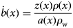
To derive accumulation rates ($\dot{b}$ ) from radar observed firn layers we use a combination of two equations following standard methods (Medley and others, Reference Medley2013; Das and others, Reference Das, Scambos, Koenig, van den Broeke and Lenaerts2015; Koenig and others, Reference Koenig2016). Equation (1) shows the w.e. accumulation rate, $\dot{b}$
 , in m w.e. a−1 at along-track location, x, using a snow density profile, ρ(x), in kg m−3, with a as the age of the layer in years from the date of radar data collection, and ρ w as the density of water in kg m−3:
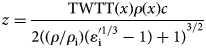
The two way travel time of the radar (TWTT) in seconds is converted to depth, z, using a dielectric mixing model for ice–air mixture from Looyenga (Reference Looyenga1965) in Eqn (2), where c is the speed of light in m s−1, ρ i is the ice density in kg m−3 and ${\varepsilon} ^{\prime}_{\rm i}$ is the dielectric permittivity of pure ice:
Equations (1) and (2) are combined to Eqn 3:
Selecting flight tracks
Any flight tracks that were included our study area, 45° W to 33° W and 60° N to 67° N, were downloaded from NSIDC and run through semiautomated layer picker software (detailed in Koenig and others, Reference Koenig2016). The flight track missions that were most often used included ‘Southeast Coastal’, ‘Southeast Glaciers’, ‘Helheim-Kangerdlugssuaq’, but vary depending on the year. Often, accumulation rates could not be derived because the layers were not clearly identifiable due to topography, flight maneuvers or meltwater percolation disrupting firn stratigraphy. There are no annual accumulation measurements available in SUMup coincident in space and time to compare with our new OIB-derived accumulation. Instead, radar-derived accumulation rates are directly compared with modeled accumulation, because our observations reflect all of the individual components of SMB throughout the winter season (when melt and runoff are absent), i.e. snowfall and sublimation/evaporation.
Density profiles and associated uncertainties
In Southeast Greenland, only 35 observed density profiles, ρ(x), are available from SUMup. Therefore, we seek to increase the coverage of this region using the FDM and Crocus firn models that have gridded density products available. A simple model, such as a semiempirical firn densification model that assumes a dry firn column, as described by Herron and Langway (Reference Herron and Langway1980), cannot be used to approximate density profiles in Southeast Greenland, because it is a region where liquid water is commonly found in the firn. To assess how these models perform and which to use for our study, we compare their output against observations at corresponding times and locations. The FDM density profiles were linearly interpolated in time to find daily values, since the original data are only output every 10 days. There is no FDM model output available beyond 2016, so an average the 2009–16 density profile was used to derive accumulation for 2017, which provides a conservative estimate. If no day was associated with the measurement in the SUMup dataset, we assigned the date to be 1st May, as in Koenig and others (Reference Koenig2016).
To determine which gridded density product to use to derive accumulation and its associated uncertainty, we examine densities from models compared with observations in the top meter and 5 m of snow across Greenland spatially. The comparison of observed and modeled density in the top meter of snow shows us how well surface processes are being represented. In the top meter across all of Greenland for 306 unique locations from the SUMup dataset (Fig. 2a), Crocus underestimates densities by 50 kg m−3, similar to the results of a 60 kg m−3 underestimation from Alexander and others (Reference Alexander, Tedesco, Koenig and Fettweis2019). In Southeast Greenland specifically, densities are being underestimated by an average of 80 kg m−3 in the top meter of firn, with an average observed value of 362 ± 45 kg m−3 and an average Crocus output value 294 ± 29 kg m−3. The FDM shows only a slight overestimation of densities within the top meter by 20 kg m−3 across all of Greenland (Fig. 2b). In Southeast Greenland, the FDM agrees well with observations, with densities overestimated by 30 kg m−3 and an average density value of 343 ± 24 kg m−3. The FDM has less variability than Crocus as well as a lower root mean squared error (RMSE) (0.06 for FDM vs 0.11 for Crocus, Fig. 2c) showing that it better represents densities in the top meter of the GrIS. However, neither model is capturing small scale variation in observed densities likely due to grid resolution (Fig. 2c). Our uncertainty is defined as the absolute difference between the modeled density and observed density in the top meter, which is determined to be 19 and 5% for Crocus and FDM, respectively. We use these errors as a measure for the final radar-derived accumulation uncertainty, because this layer comprises most (if not all) of the winter accumulation.
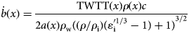
Further, we analyze the density profiles of both observations and models to the depth of the highest radar-derived accumulation rates we have observed, ~5 m snow w.e. The average density of the top 5 m of snow/firn from SUMup observations in Southeast Greenland (representing 35 unique cores) is 437 ± 59 kg m−3 (Fig. 3). Below the top meter in Crocus, the densification rate slows because there is less pore space available to compact and it is compensating for the excessive densification rate above. This compensation of density values allows Crocus to have a low bias for the top 5 m with an average value of 432 ± 90 kg m−3. The FDM density profile agrees better with the observations overall, showing a similar densification rate, although it still slightly underestimates the average density values (404 ± 50 kg m−3). We use the FDM density profiles to derive accumulations and in our analysis because they are within the uncertainty range of the observations, i.e. ±1 std dev., though we also derive accumulations using the Crocus profiles only to quantify the total uncertainty.
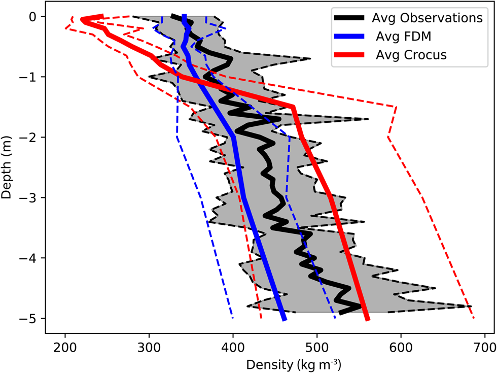
Fig. 3. Average density profile of the top 5 m of all observed SUMup (N = 35) cores (black) in Southeast Greenland and co-located FDM (blue), and Crocus (red) in space and time. The std dev. is shown in the dashed line of the same color.
Determining layer age and total accumulation uncertainty
Depth or layer ages, a, are determined by assuming that spatially continuous isochronal layers are annually resolved. An automated layer picker (Koenig and others, Reference Koenig2016) was used to find the peak density gradients to determine layer ages that were verified and adjusted manually as necessary using a graphical user interface. The first layer would represent 10 months instead of the full year in our study. This is because it encompasses the springtime measurement from the snow radar aboard OIB (often taken in April/May) back to the previous year's melt, causing a peak in the density gradient in July ± 1 month (Koenig and others, Reference Koenig2016). The second source of error occurs during manual adjustment of the picked layers and is estimated to be a maximum of ±3 range bins, or ~8 cm (Koenig and others, Reference Koenig2016). In our study, this accounts for a range of 7–13% errors (10% on average) depending on accumulation rates, which is similar to the mean error of 7% found in Koenig and others (Reference Koenig2016). Combining this with the errors from the density models we get a total error range on the radar-derived accumulation of 11% (FDM) to 21% (Crocus) depending on the firn model used. The results we show are only representative of the radar-derived accumulations using the FDM density profiles.
Results
Radar-derived accumulation rates
A time series of accumulation rates and their uncertainties were derived from OIB snow radar from 2009 to 2017 (Fig. 4). Average radar-derived accumulation across all of Southeast Greenland for each year ranges from 0.5 to 1.2 m w.e. with higher values near the coast and decreasing values as you move inland. The year-to-year variable acquisition of observations is due to the variations in flight lines and data quality. An increase in spatial coverage from 2009 to 2011 can be explained by a greater number of flights and adjustments to the radar antenna leading to better data quality (Koenig and others, Reference Koenig2016). Resulting from the improved data quality, the percentage of measurements that were able to be derived from all flight lines increased from ~40 to 70% in those years. From 2012 to 2014, there was less coverage, with only one flight line obtained in 2013 and three in 2014, likely due to unfavorable flying conditions in those seasons, along with only ~22–46% of the data of sufficient quality. Years 2015 and 2017 provide more complete spatial coverage, with more consistent flight paths as well as ~58–65% of the radar data containing discernible layers. In 2016, there was reduced radar performance on many flights leading to a lack of quality data (36%). The number of flights and area covered varies by year (Supplementary Table 1, Fig. 4), with peak coverage in 2011 (70%) and 2015 (65%).
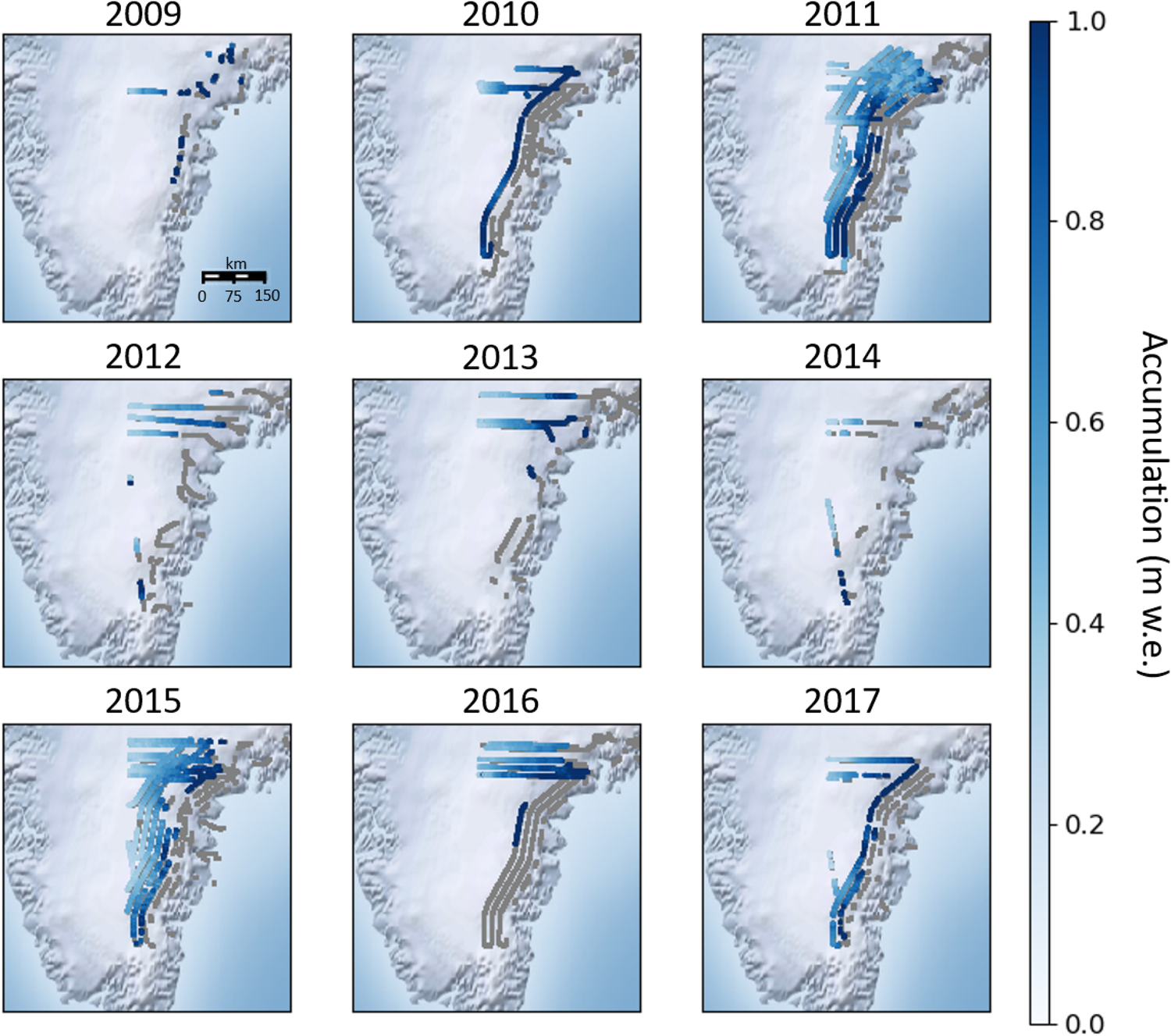
Fig. 4. Annual accumulation (m w.e.) derived from OIB snow radar, from 2009 to 2017. Flight tracks that were not discernible for accumulation layers are shown in gray.
Comparison with RCMs: interannual variability
With a dataset of radar-derived accumulation rates spanning almost 10 years, we can analyze the interannual variability and compare that with RCMs (Fig. 5). Since there is no single OIB flight line that is consistently flown every year from 2009 to 2017, we focus our analysis on an area (45° W to 41° W and 66.3° N to 66.55° N, Fig. 1) that contains a partial set of flight lines each year (except for 2009), and match these observations in space and time with the closest MAR and RACMO2 grid points. Accumulation from RACMO2 follows a similar pattern of interannual variations, although it had a relatively large bias of −0.18 m w.e (44%). In contrast, MAR shows a more constant accumulation rate from 2010 to 2017. However, its multi-annual mean is closer to the observations, with an average bias of −0.13 m w.e. (29%). Over this time period, RACMO2 captures the interannual trends (r 2 = 0.86) while MAR does not (r 2 = 0.08), showing very little interannual variability. To assess how representative the 2010–17 period is for the longer-term accumulation record (1979–2017), and considering the above model biases, we analyze the 30-year mean and variability in accumulation across the same area from RCMs (Fig. 5b). For both RACMO2 and MAR, the std dev. of the 2010–17 accumulation (RACMO2: 0.408 ± 0.039; MAR: 0.45 ± 0.024) fall within the 1979–2017 variability (RACMO2: 0.43 ± 0.063; MAR: 0.47 ± 0.068). This implies that the RCM analysis in this study area is consistent with interannual patterns spanning multiple decades.
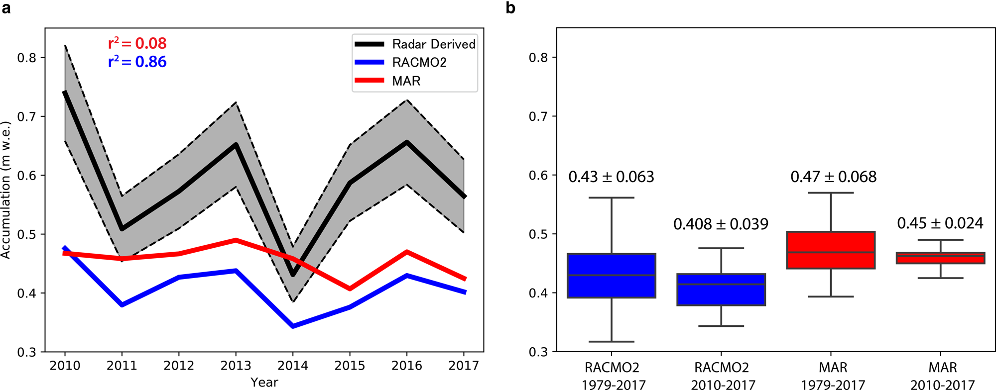
Fig. 5. (a) Inter-annual variability of radar-derived accumulation rates (black) from 2010 to 2017 of area overflown each year compared with MAR (red) and RACMO2 (blue). Uncertainty of observations (11%) shown in dashed lines of the same color. (b) Box plot of RACMO2 and MAR accumulations from 1979 to 2017 showing the middle 50% of data (second and third quartiles), the line inside the box represents the median values, and the whiskers show the greatest/least values within 1.5 times the interquartile range of the upper and lower quartiles.
Comparison with RCMs: spatial variability
Radar-derived accumulation rates from each 10-month period were compared with downscaled 1 km MAR and RACMO2 accumulation covering the same period. The years of 2011 and 2015 had the best spatial coverage and are shown in Figure 6i. RACMO2 underestimates accumulation rates in Southeast Greenland with a mean bias of −0.51 m w.e. across the entire region in 2011 and −0.41 m w.e. in 2015. In 2011, accumulation is overestimated toward the lower elevations (<1500 m) but this is dominated by accumulation underestimation everywhere else. MAR closely matches accumulation rates in 2011 with a mean bias of −0.09 m w.e. and in 2015 the mean bias is −0.22 m w.e. averaged across Southeast Greenland. This good agreement in 2011 reflects the low spatial heterogeneity compared with observations. Scatterplots show a similar pattern to the difference plots, showing that both MAR and RACMO2 underestimate accumulation in Southeast Greenland (Fig. 6ii). The RMSE for RACMO2 during 2011 (0.26) and 2015 (0.29) are greater than those from MAR for the same years (0.17 and 0.23). When considering the 11% uncertainty of the radar-derived accumulation, the RMSE of each year decreases, except for MAR in 2011 where the RMSE is the same (RACMO2 2011: 0.18, RACMO2 2015: 0.12; MAR 2011: 0.17, MAR 2015: 0.08). However, the uncertainty does not fully account for the difference in radar-derived vs modeled accumulation and therefore it must be attributed to a physical process in the models.
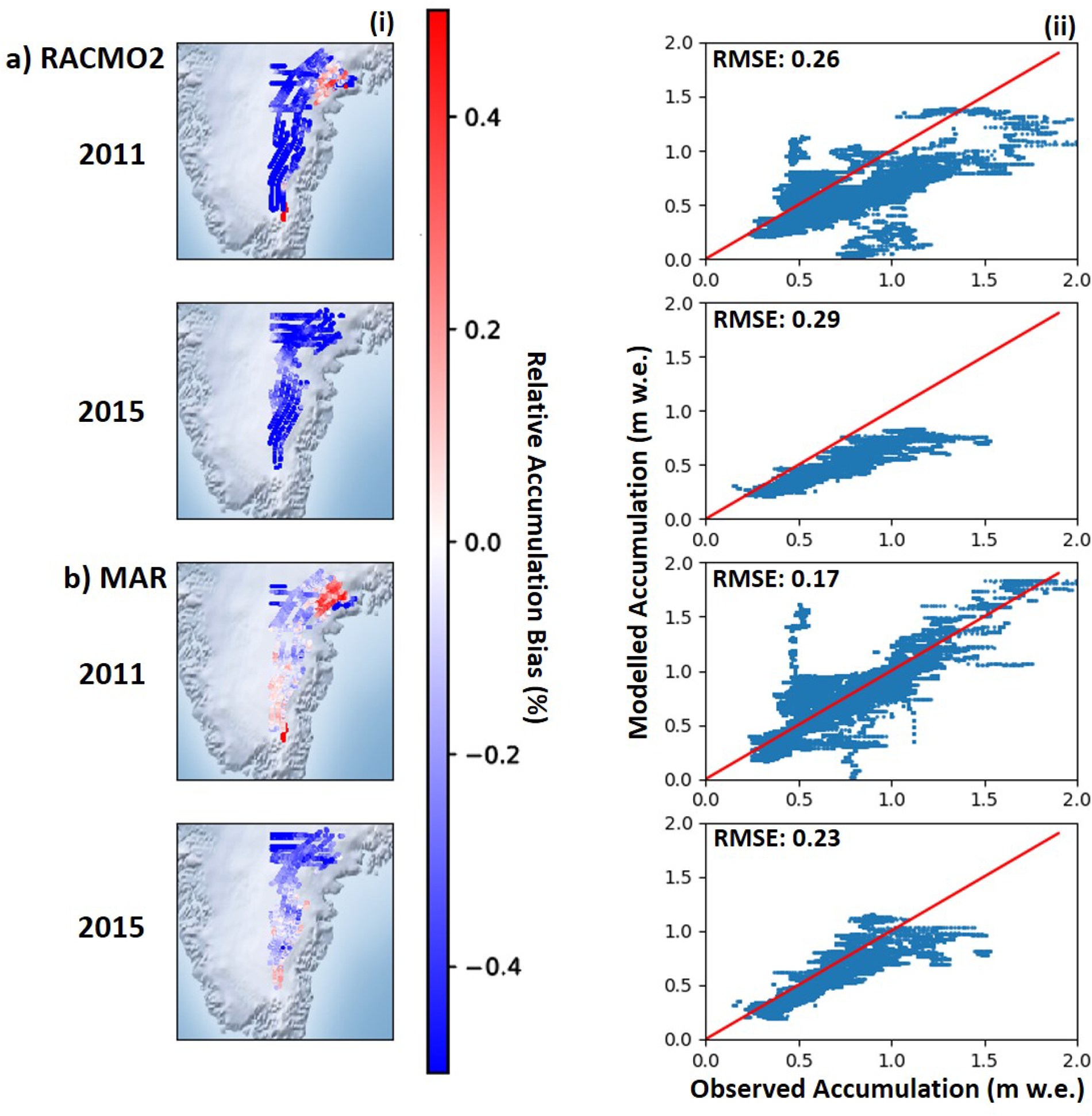
Fig. 6. (a) (i) Relative difference between OIB derived accumulation and RACMO2 for 2011 and 2015, and (ii) scatterplots showing radar-derived accumulation vs RACMO2. (b) The same analysis except with MAR.
Discussion
Annual accumulation can be derived from OIB-airborne radar in Southeast Greenland. However, in general, only the most recent layer or ~10 months can be detected in the percolation zone where melt and refreezing obscures the stratigraphy below the last year's snowfall. A future increase and inland progression of surface melt on the GrIS implies that this technique's potential to yield reliable long-term accumulation records will be progressively more challenging in the future. We can reduce the spatial uncertainty of these derived measurements by attaining more in situ observations along OIB flight-line tracks.
This study provides a record of OIB radar-derived accumulation in Southeast Greenland that has been extended from Koenig and others (Reference Koenig2016) to include 2009 to 2017. Compared with that earlier study, we have also updated some of the methods and datasets. First, we use an updated version of MAR (v3.9.2) as well as RACMO2 to compare RCM accumulation with OIB radar-derived accumulation. Second, we use FDM density profiles to derive accumulation, which best represent Southeast Greenland. The resulting differences between our results and Koenig and others (Reference Koenig2016) illustrate that realistic density profiles are essential to convert radar-derived depth to accumulation. This is highlighted by our comparison of Crocus and FDM with observations, yielding a total uncertainty associated only with a density choice of 5% (FDM) to 19% (Crocus). The FDM density profiles show better agreement with observations, likely because the FDM physics are designed for use over ice sheets, while the Crocus model is developed for Alpine snow conditions. FDM profiles are also tuned to measurements from the GrIS (Kuipers Munneke and others, Reference Kuipers Munneke2015). Along with the density estimate, layer picking software is a source of uncertainty in deriving accumulation rates and has been quantified by Koenig and others (Reference Koenig2016) to be ~8 cm from manual adjustment of layers or an average of 10% uncertainty in our study. Our overall uncertainty of 11% on radar-derived accumulation is reasonable compared with other studies, which yield uncertainties of 14–15% (Medley and others, Reference Medley2013; Koenig and others, Reference Koenig2016). The biases between models and observations as well as the uncertainties can be constrained by collecting additional coincident observations of accumulation and density in Southeast Greenland. These observations are also necessary to provide an independent estimate of Southeast Greenland accumulation, as RCMs are currently the only tool available to provide GrIS SMB at this spatial resolution.
To assess future changes in accumulation and SMB, we must be able to differentiate between interannual variability and longer-term trends in RCMs. Interannual variability of accumulation in Southeast Greenland is driven by synoptic patterns associated with the strength and location of the Icelandic Low situated to the east of Greenland (Berdahl and others, Reference Berdahl2018). On average, the large-scale southwesterly atmospheric circulation brings moisture to the southern coast of Greenland, where the steep slopes of the ice sheet act as efficient barriers to the flow, and orographic precipitation is abundant. Over the 2010–17 time period (2009 is excluded because no flight lines overlap our case study region in that year), our case study shows that RACMO2 captures the interannual trends better than MAR, while MAR better represents the absolute magnitude of radar-derived accumulation. Over a 30 year period from 1979 to 2017, accumulation is examined from MAR and RACMO2 to show that variability of the study period (2010–17) is within that of the longer-term from both RCMs (Fig. 5b). On the other hand, the 8-year time period we observe is too short to discern a significant long-term trend. We would need OIB data from a longer time period, similar to that of the RCMs (>30 years), to attempt to isolate long-term trends from interannual variability.
In order to quantify how much accumulation Southeast Greenland contributes to the GrIS's total SMB, and how it may impact changes in SMB in the future, spatial variability of accumulation in RCM's is vital to understand. When comparing modeled mean bias with observations in our flight-line case study (Fig. 5a), accumulation is underestimated by both MAR and RACMO2. This result could be due to the specific to this study area chosen, and unfortunately we are unable to expand this assessment to other regions, since this is the only region that has coverage in most years. However, our comparison of the spatial variability in models and observations (Fig. 6i) suggests that this result is valid for the larger Southeast Greenland region. As other SMB components (including melt, sublimation and blowing snow redistribution) are at least two orders of magnitudes smaller than snowfall (mm vs m) in Southeast Greenland (Box and Steffen, Reference Box and Steffen2001; Lenaerts and others, Reference Lenaerts, van den Broeke, van Angelen, van Meijgaard and Déry2012), the biases in the RCMs must be attributed to biases in snowfall.
RACMO2 has a high snowfall bias near the coast, while MAR has a larger bias in the interior (Fig. 7). These patterns are consistent with the relative differences shown in Figure 6, where RACMO2 shows underestimation inland and MAR shows an overestimation. Our MAR results contrast with those of Koenig and others (Reference Koenig2016), who found that an earlier version of MAR (MAR3.5.2) overestimated accumulation in all of Southeast Greenland. With updated physics (increase in the cloud life time (Fettweis and others, Reference Fettweis2017; Delhasse and others, Reference Delhasse, Fettweis, Kittel, Amory and Agosta2018) and employed at higher resolution (15 vs 25 km)), MARv3.9 shows good agreement across most of the region, though still slightly underestimates accumulation. The majority of the radar-derived accumulations are taken closer inland than where RACMO2 has dominant snowfall events, closer to the coast (Fig. 7). These biases are due to the fact that we are working with model accumulation downscaled to 1 km, which better resolves accumulation than the original grids, but still cannot take into account the mountainous topography in Southeast Greenland. The bias toward higher snowfall on the coast in RACMO2 is likely due to the representation of orographic precipitation in the model, i.e. when moist easterly air masses collides with coastal mountains and precipitate as they are lifted, resulting in high coastal precipitation and drier conditions further inland. RACMO2 resolves topographical features that have to do with orographic precipitation, while MAR cannot, because downscaled 1 km RACMO2 has a higher original horizontal resolution (5.5 km) than downscaled 1 km MAR (15 km).
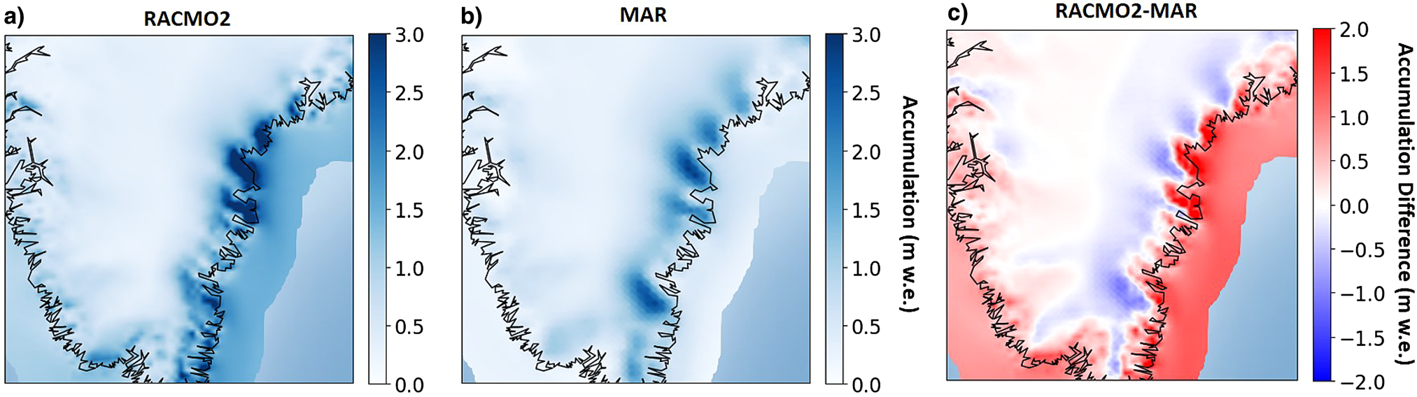
Fig. 7. Average annual snowfall (m w.e.) from 2009 to 2017 in (a) RACMO2, (b) MAR and (c) RACMO2–MAR.
Our results corroborate previous work, which has shown that RACMO2 overestimates accumulation at lower elevations and MAR overestimates accumulation at higher elevations. On the Q-transect on the Qagssimiut ice lobe in South Greenland, RACMO2 shows a wet bias toward the coast that is likely the dominant source of error (Hermann and others, Reference Hermann2018). Similarly, in RACMO2, Antarctica has a bias of orographic precipitation in coastal areas, likely because it does not compute precipitation prognostically (i.e. snow falls in the same gridcell that it is created) (Lenaerts and others, Reference Lenaerts2018). Schmidt and others (Reference Schmidt2018) emphasized the same concern about overestimation of accumulation due to high orographic forcing in RCMs and attributes some of the error to the precipitation scheme in hydrostatic models, recommending the use of WRF or HARMONIE as a non-hydrostatic alternative. Our results further verify these model biases, leading to the conclusion that RCMs must be improved to be better representative of the current climatological conditions since observations will continue to be sparse across the majority of the ice sheet. We propose future work of comparing radar-derived accumulations using a diagnostic, non-hydrostatic, high resolution model to diagnose the different precipitation schemes and see if we can reduce the error in accumulation. Additionally, we recommend that model development target orographically forced precipitation at the coast, as it is a large source of error in SMB calculations that could influence total SMB of the GrIS.
Conclusions
A dataset of annual accumulation was derived from OIB snow radar for 2009–17 in Southeast Greenland where there were very few in situ measurements available. Our estimated uncertainty of this new dataset is 11%, which results from the uncertainty associated with semiautomated layer picking software, and uncertainty in the FDM density profiles used to derive the accumulation. We find that density profiles vary widely in the top meter of firn and can widely affect accumulation rates, especially in the high-accumulation area of Southeast Greenland. This dataset can be used to validate RCMs in Southeast Greenland, an area of high variability and uncertainty. RACMO2 consistently underestimates accumulation rates across the entire region in 2011 and 2015 (the years with the best spatial coverage), but was able to capture interannual variability in a case study region. MAR shows better agreement with accumulation rates in 2011 and 2015 across Southeast Greenland, though shows little interannual variability. The pattern observed in the relative differences can be explained by the snowfall component of each model which is biased higher toward the coast in RACMO2 and inland in MAR. In situ observations in this region will always be sparse, so we must rely on RCMs in the future to assess changing SMB. This study points to the need of focused model development of precipitation schemes to more accurately portray high accumulation regions on the GrIS.
Supplementary material
The supplementary material for this article can be found at https://doi.org/10.1017/aog.2020.8
Data
This new accumulation dataset is available at the Arctic Data Center (doi: https://doi.org/10.18739/A2J96095Z).
Acknowledgements
Lynn Montgomery and Lora Koenig acknowledge the National Science Foundation (PLR 1603407) and the NASA Earth and Space Science Fellowship (80NSSC17K0383). Peter Kuipers Munneke is funded by the Netherlands Earth System Science Centre (NESSC). We thank Xavier Fettweis for assistance with MAR model output and Brice Noël for discussion about RACMO2 output. We also thank the Associate Chief Editor Dustin Schroeder, the Scientific Editor Michelle Koutnik, and the two anonymous reviewers for their comments and suggestions, which greatly helped us in improving our paper.


 Open access