


1 Introduction
With the development of risk management strategies, the study of optimal reinsurance has been explored from many different perspectives. Insurers would like to buy reinsurance contracts to protect themselves from large losses. Reinsurers receive premiums from the insurers and earn profits by undertaking risks. In the literature of optimal reinsurance, different premium principles and optimality criteria have been considered to explore the optimal structure of reinsurance contracts from the insurers’ point of view. However, there has been little research investigating the optimal reinsurance from the reinsurer’s perspective. In this paper, we fill that gap by deriving optimal safety loading of reinsurance contracts from the reinsurer’s perspective.
In the early age of the research in optimal reinsurance, researchers tried to find the optimal form of reinsurance contract within the expected utility framework, which is based on the assumption that the decision makers will always try to maximise their expected utility. Borch (Reference Borch1960) and Arrow (Reference Arrow1963) investigated the problem under the expectation premium principle by maximising the expected utility of the reinsurer’s wealth, and they concluded that stop-loss reinsurance is optimal. Recently, Guerra & Centeno (Reference Guerra and Centeno2008) considered the optimal reinsurance from the cedent company’s perspective to derive the optimal form by studying the relationship between maximising the adjustment coefficient and maximising the expected utility. The authors assumed that the premium principle is a convex functional, and the results show that both stop-loss reinsurance contract and a formulated non-linear function could be optimal under different premium principles.
In Cai & Tan (Reference Cai and Tan2007), the authors derived the optimal retention for a stop-loss reinsurance under the value-at-risk (VaR) and conditional tail expectation (CTE) risk measures. In Cai et al. (Reference Cai, Tan, Weng and Zhang2008), the optimal reinsurance problem from the insurers’ perspective was reconsidered and the optimal ceded loss functions were derived using the VaR and CTE risk measures. The results show that the optimal ceded loss function only depends on the insurer’s risk tolerance level and the safety loading of the reinsurance, and the optimal reinsurance contract could be in the form of stop-loss, quota-share and change-loss under different conditions. We now describe their model and result here.
Let X be the initial loss of the insurer, which is an integrable non-negative random variable. We assume that its survival function S
X
is strictly decreasing and continuous on (0, ∞), with a possible jump at 0. We also assume
 $$f\,\colon\,\def\Bbb{\tf="Macopen"} {\Bbb R}^{\!{\plus}}\!\!\to\!{\Bbb R}^{\!{\plus}} $$
is the ceded loss function, so that f(x) is the amount of money that the reinsurer has to pay to the insurer when the insurer suffers loss x. It is required that f(x) is increasing, convex, and 0≤f(x)≤x for all x. The collection of all such functions is denoted as
$$f\,\colon\,\def\Bbb{\tf="Macopen"} {\Bbb R}^{\!{\plus}}\!\!\to\!{\Bbb R}^{\!{\plus}} $$
is the ceded loss function, so that f(x) is the amount of money that the reinsurer has to pay to the insurer when the insurer suffers loss x. It is required that f(x) is increasing, convex, and 0≤f(x)≤x for all x. The collection of all such functions is denoted as
 $${\cal F}$$
.
$${\cal F}$$
.
Let δ
f,ρ
(X) be the associated reinsurance premium, where
 $$f\!\!\in\!{\cal F}$$
and ρ>0 is the safety loading. Here we suppose that ρ is a constant determined by the reinsurer. Following Cai et al. (Reference Cai, Tan, Weng and Zhang2008), we suppose that expectation premium principle holds so that
$$f\!\!\in\!{\cal F}$$
and ρ>0 is the safety loading. Here we suppose that ρ is a constant determined by the reinsurer. Following Cai et al. (Reference Cai, Tan, Weng and Zhang2008), we suppose that expectation premium principle holds so that
 $$\delta _{{f,\rho }} \left( X \right)\,{\equals}\,\left( {1{\plus}\rho } \right)\def\Bbb{\tf="Macopen"}{\Bbb E}\left[ {f\left( X \right)} \right]$$
. The retained loss of the insurer is I
f
(X)=X−f(X), and the total loss of the insurer is T
f
(X)=I
f
(X)+δ
f,ρ
(x). In order to be consistent with the aforementioned literature, we simplify the notations by introducing the following taken from Cai et al. (Reference Cai, Tan, Weng and Zhang2008) and Cheung (Reference Cheung2010):
$$\delta _{{f,\rho }} \left( X \right)\,{\equals}\,\left( {1{\plus}\rho } \right)\def\Bbb{\tf="Macopen"}{\Bbb E}\left[ {f\left( X \right)} \right]$$
. The retained loss of the insurer is I
f
(X)=X−f(X), and the total loss of the insurer is T
f
(X)=I
f
(X)+δ
f,ρ
(x). In order to be consistent with the aforementioned literature, we simplify the notations by introducing the following taken from Cai et al. (Reference Cai, Tan, Weng and Zhang2008) and Cheung (Reference Cheung2010):
 $$\rho ^{{\asterisk}} \,\colon\!{\equals}\,{1 \over {1{\plus}\rho }},\,d^{{\asterisk}} \,\colon\!{\equals}\, S_{X}^{{{\minus}1}} \left( {\rho ^{{\asterisk}} } \right)$$
 $$g(x)\,\colon\!{\equals}\,x{\plus}{1 \over {\rho ^{{\asterisk}} }}{\int}_x^\infty S_{X} (t)dt$$
 $$u(x)\,\colon\!{\equals}\,S_{X}^{{{\minus}1}} (x){\plus}{1 \over {\rho ^{{\asterisk}} }}{\int}_{S_{X}^{{{\minus}1}} (x)}^\infty S_{X} (t)dt$$
 $$a\,\colon\!{\equals}\,S_{X}^{{{\minus}1}} (\alpha )$$
Finally, we assume that 0<α<S X (0). Because when α≥S X (0), we obtain VaR X (α)=0, which is trivial.
The optimal reinsurance problems based on VaR and CTE risk measures can be stated as follows:
VaR-minimisation problem:
 $$\:{\rm VaR}_{{T_{{f^{{\asterisk}} }} \left( X \right)}} (\alpha )\,{\equals}\,\mathop {{\rm min}}\limits_{f\in{\cal F}} \big\{ {{\rm VaR}_{{T_{{f(X)}} }} (\alpha )} \big\}$$
CTE-minimisation problem:
 $$\:{\rm CTE}_{{T_{{f^{{\asterisk}} }} (X)}} \left( \alpha \right)\,{\equals}\,\mathop {{\rm min}}\limits_{f\in{\cal F}} \:\big\{ {{\rm CTE}_{{T_{{f(X)}} }} \left( \alpha \big)} \right\}$$
The following theorem, taken from Cheung (Reference Cheung2010), described the solutions to the above VaR-minimisation problem.
Theorem 1 For a given α∈(0, S X (0)), the following statements hold true:
-
(a) If ρ*<S X (0) and a>u(ρ*), the optimal ceded loss function is f*(x)=(x−d*)+.
-
(b) If ρ*<S X (0) and a=u(ρ*), the optimal ceded loss function is f*(x)=c(x−d*)+ for any constant c∈[0, 1].
-
(c) If ρ*≥S X (0) and a>g(0), the optimal ceded loss function is f*(x)=x.
-
(d) If ρ*≥S X (0) and a=g(0), the optimal ceded loss function is f*(x)=cx for any constant c∈[0, 1].
-
(e) For all other cases, the optimal ceded loss function is f*(x)≡0.
Extensive research has been conducted following Cai et al. (Reference Cai, Tan, Weng and Zhang2008) from insurers’ perspective, for example, see Bernard & Tian (Reference Bernard and Tian2009), Tan et al. (Reference Tan, Weng and Zhang2011), Chi & Lin (Reference Chi and Lin2014) and Cheung et al. (Reference Cheung, Sung, Yam and Yung2014). In this paper, it is assumed that the insurer will choose the form of the reinsurance contract by following the results derived in Cai et al. (Reference Cai, Tan, Weng and Zhang2008). By applying optimality criteria from the reinsurer’s perspective, the optimal safety loading that the reinsurer should set in the reinsurance pricing is studied, which is novel in the literature. The paper is organised as follows. In section 2, we derive the optimal safety loading of the reinsurance contracts with the assumption that the reinsurer only faces one risk. In section 3, we generalise the model in section 2 from one risk to two risks. In section 4, two numerical examples are provided to illustrate the results derived in sections 2 and 3. In section 5, we make a conclusion for this paper and indicate some possible applications as well as further research directions.
2 Optimal Safety Loading with One Risk
2.1 Introduction
Suppose that the reinsurer is facing one risk (one insurer) only, and this single insurer will apply Theorem 1 to choose the optimal function f* as the reinsurance contract. In this case, we have to derive five different cases for the value range of the safety loading based on the inequalities stated in Theorem 1. For each case, the insurer chooses the relative ceded loss function to cover part of its loss. Three optimisation models from the reinsurer’s point of view: maximising expected profit, maximising expected utility and minimising VaR of the total loss, will be established and the optimal safety loading for each model will be derived based on the five cases. Here we assume that the initial loss of the insurer X follows a zero-modified exponential distribution with survival function S X (t)=γe −λt , λ>0, 0<γ<1, t>0. The motivation to have that assumption is that if the claims are assumed to be independent and identically distributed random variables with common exponential distribution and the number of the claims is geometric distributed, then the initial loss of the insurer, which is the sum of the claims, can be proved to be zero-modified exponential distributed. For detailed proof, we refer to Panjer & Willmot (Reference Panjer and Willmot1992). Closed-form results can also be obtained when the loss follows other distributions, for example, the zero-modified Pareto distribution assumption, see Appendix A for more details.
2.2 The value range of the safety loading
Case 1: If the insurer would like to choose the stop-loss reinsurance in the form of f(x)=(x−d*)+, according to Theorem 1 (a), the safety loading ρ has to fulfil the following two conditions:
-
i. ρ*<S X (0). Then we have
(1) $$\rho \,\gt\,{1 \over \gamma }{\minus}1$$
-
ii. a>u(ρ*). We derive

 $$a\,\gt\,u\left( {\rho ^{{\asterisk}} } \right)\Leftrightarrow\rho \,\lt\,{1 \over \gamma }e^{{a\lambda {\minus}1}} {\minus}1$$
From (1) and (2) we have the following conclusion.
-
∙ If aλ≤1, ρ does not exist.
-
∙ Otherwise, if aλ>1, we have
$$\rho \in\big( {{1 \over \gamma }{\minus}1,{1 \over \gamma }e^{{a\lambda {\minus}1}} {\minus}1} \big)$$
.
So in Case 1 we only need to consider the situation where aλ>1.
Case 2: If the insurer would like to choose the change-loss reinsurance in the form of f(x)= c(x−d*)+, c∈[0, 1], according to Theorem 1 (b), the safety loading ρ has to fulfil the following two conditions:
-
i. ρ*<S X (0) and we have the following result which is the same with that in Case 1:
(3)
$$\rho \,\gt\,{1 \over \gamma }{\minus}1$$
-
ii. a=u(ρ*), from which we can derive the value range of ρ as follows by applying the result in Case 1:

 $$\rho \,{\equals}\,{1 \over \gamma }e^{{a\lambda {\minus}1}} {\minus}1$$
From (3) and (4) we obtain the following conclusion:
-
∙ If aλ≤1, ρ does not exist.
-
∙ Otherwise, if aλ>1, we have
$$\rho \,{\equals}\,{1 \over \gamma }e^{{a\lambda {\minus}1}} {\minus}1$$
.Again, in Case 2 we only need to consider the situation when aλ>1.
Case 3: If the insurer would like to choose the full reinsurance in the form of f(x)=x, according to Theorem 1 (c), the safety loading ρ has to fulfil the following two conditions:
-
i. ρ*≥S X (0), and we have the following deduction:
(5)
$$\rho \leq {1 \over \gamma }{\minus}1$$
-
ii. a>g(0), and we have the following deduction:
-


 $$\rho \,\lt\,{{a\lambda } \over \gamma }{\minus}1$$
Combining (5) and (6), we conclude that
-
∙ If aλ>1, we have
$$0\,\lt\,\rho \leq {1 \over \gamma }{\minus}1$$
. -
∙ If γ<aλ≤1, we have
$$0\,\lt\,\rho \,\lt\,{{a\lambda } \over \gamma }{\minus}1$$
. -
∙ Otherwise aλ≤γ, we have
$$\rho \,\lt\,{{a\lambda } \over \gamma }{\minus}1\leq 0$$
, which is impossible.Therefore, in Case 3 we only consider the situation when γ<aλ.
Case 4: If the insurer would like to choose the quota-share reinsurance in the form of f(x)=cx, c∈[0, 1], according to Theorem 1 (d), the safety loading ρ has to fulfil the following two conditions:
-
i. ρ*≥S X (0). By applying the result derived in Case 3, we have
(7)
$$\rho \leq {1 \over \gamma }{\minus}1$$
-
ii. a=g(0), and we have the following deduction.
-


 $$\rho \,{\equals}\,{{a\lambda } \over \gamma }{\minus}1$$
From (7) and (8) we have the following results.
-
∙ If aλ>1, ρ does not exist.
-
∙ If γ<aλ≤1, we have
$$\rho \,{\equals}\,{{a\lambda } \over \gamma }{\minus}1$$
-
∙ Otherwise, if aλ≤γ, we have
$$\rho \,{\equals}\,{{a\lambda } \over \gamma }{\minus}1\leq 0$$
, which is impossible.


Hence in Case 4 we only consider the situation when γ<aλ≤1.
Case 5: According to Theorem 1 (e), for all other cases, the optimal ceded loss function is given by f*(x)≡0.
2.3 Optimisation models
2.3.1 Maximising the expected profit of the reinsurer
We denote the profit of the reinsurer by A, so that
 $$A{\equals}\,(1{\plus}\rho )\def\Bbb{\tf="Macopen"}{\Bbb E}[f(X)]{\minus}f(X)$$
Denote the objective function of this model by
 $$l(\rho )\,{\equals}\,\def\Bbb{\tf="Macopen"}{\Bbb E}[A]{\equals}\,\rho {\Bbb E}[f(X)]$$
Then the optimal reinsurance problem can be stated as
 $$\mathop {{\rm max}}\limits_\rho l(\rho ){\equals}\,\mathop {{\rm max}}\limits_\rho \rho \def\Bbb{\tf="Macopen"}{\Bbb E}[f(X)]$$
We remark that f in (9) implicitly depends on ρ as described by Theorem 1, so that l(ρ) is indeed a complicated non-linear function of ρ.
We now apply the results about the value range of the safety loading ρ derived in section 2.2 and solve the optimisation problem (9) accordingly.
Case 1: For aλ>1, we have
 $$\rho \in\big( {{1 \over \gamma }{\minus}1,{1 \over \gamma }e^{{a\lambda {\minus}1}} {\minus}1} \big)$$
and the ceded loss function should be f(x)=(x−d*)+. we can write the objective function in this case as
$$\rho \in\big( {{1 \over \gamma }{\minus}1,{1 \over \gamma }e^{{a\lambda {\minus}1}} {\minus}1} \big)$$
and the ceded loss function should be f(x)=(x−d*)+. we can write the objective function in this case as
 $$l_{1} (\rho ){\equals}\,\rho \def\Bbb{\tf="Macopen"}{\Bbb E}\left[ {X\,{\minus}\,d^{{\asterisk}} } \right]_{\!{\plus}} {\equals}\,{\rho \over {\lambda (1{\plus}\rho )}}$$
where we can see l
1(ρ) is increasing and concave over ρ. Hence l
1(ρ) will go to its supremum value as ρ goes to
 $${1 \over \gamma }e^{{a\lambda {\minus}1}} {\minus}1$$
. Since ρ cannot reach
$${1 \over \gamma }e^{{a\lambda {\minus}1}} {\minus}1$$
. Since ρ cannot reach
 $${1 \over \gamma }e^{{a\lambda {\minus}1}} {\minus}1$$
, the maximum of l
1(ρ) cannot be achieved. Thus
$${1 \over \gamma }e^{{a\lambda {\minus}1}} {\minus}1$$
, the maximum of l
1(ρ) cannot be achieved. Thus
 $$l_{1} (\rho )\in\left( {{{1{\minus}\gamma } \over \lambda },{1 \over \lambda }{\minus}{\gamma \over \lambda }e^{{1{\minus}a\lambda }} } \right)$$
, where
$$l_{1} (\rho )\in\left( {{{1{\minus}\gamma } \over \lambda },{1 \over \lambda }{\minus}{\gamma \over \lambda }e^{{1{\minus}a\lambda }} } \right)$$
, where
 $$\rho \in\big( {{1 \over \gamma }{\minus}1,{1 \over \gamma }e^{{a\lambda {\minus}1}} {\minus}1} \big)$$
. To conclude, we have
$$\rho \in\big( {{1 \over \gamma }{\minus}1,{1 \over \gamma }e^{{a\lambda {\minus}1}} {\minus}1} \big)$$
. To conclude, we have
 $$\mathop {{\rm sup}\,}\limits_\rho l_{1} (\rho )\,{\equals}\,{1 \over \lambda }{\minus}{\gamma \over \lambda }e^{{1{\minus}a\lambda }} $$
 $${\rm as}\quad \rho \nearrow{1 \over \gamma }e^{{a\lambda {\minus}1}} {\minus}1$$
Case 2: For aλ>1, we have
 $$\rho \,{\equals}\,{1 \over \gamma }e^{{a\lambda {\minus}1}} {\minus}1$$
and the ceded loss function should be f(x)=c(x−d*)+, c∈[0.1]. We write the objective function in this case as
$$\rho \,{\equals}\,{1 \over \gamma }e^{{a\lambda {\minus}1}} {\minus}1$$
and the ceded loss function should be f(x)=c(x−d*)+, c∈[0.1]. We write the objective function in this case as
 $$l_{2} (\rho )\,{\equals}\,cl_{1} (\rho )\,{\equals}\,c\rho \def\Bbb{\tf="Macopen"}{\Bbb E}\left[ {X{\minus}d^{{\asterisk}} } \right]_{{\plus}} {\equals}\,{{c\rho } \over {\lambda (1{\plus}\rho )}}$$
In this case, the safety loading ρ has only one possible value, so we have the maximum l 2(ρ) as follows:
 $$\mathop {{\rm max}\,}\limits_\rho l_{2} (\rho )\,{\equals}\,c\left( {{1 \over \lambda }{\minus}{\gamma \over \lambda }e^{{1{\minus}a\lambda }} } \right)$$
 $${\rm at}\;\;\rho \,{\equals}\,{1 \over \gamma }e^{{a\lambda {\minus}1}} {\minus}1$$
Now we compare the supremum or maximum values in Case 1 and Case 2. In both cases we have aλ>1, and c∈[0, 1], so
 $$c\left( {{1 \over \lambda }{\minus}{\gamma \over \lambda }e^{{1{\minus}a\lambda }} } \right)\leq {1 \over \lambda }{\minus}{\gamma \over \lambda }e^{{1{\minus}a\lambda }} $$
. Then we obtain that
$$c\left( {{1 \over \lambda }{\minus}{\gamma \over \lambda }e^{{1{\minus}a\lambda }} } \right)\leq {1 \over \lambda }{\minus}{\gamma \over \lambda }e^{{1{\minus}a\lambda }} $$
. Then we obtain that
 $$\mathop {{\rm max}\,}\limits_\rho l_{2} (\rho )\leq \mathop {{\rm sup}}\limits_\rho \,l_{1} (\rho )$$
Case 3: If aλ>1, we have
 $$0\,\lt\,\rho \leq {1 \over \gamma }{\minus}1$$
. If γ<aλ≤1, we have
$$0\,\lt\,\rho \leq {1 \over \gamma }{\minus}1$$
. If γ<aλ≤1, we have
 $$0\,\lt\,\rho \,\lt\,{{a\lambda } \over \gamma }{\minus}1$$
. The ceded loss function chosen by the insurer in this case is given by f(x)=x, x≥0. We can write the objective function in this case as
$$0\,\lt\,\rho \,\lt\,{{a\lambda } \over \gamma }{\minus}1$$
. The ceded loss function chosen by the insurer in this case is given by f(x)=x, x≥0. We can write the objective function in this case as
 $$l_{3} (\rho ){\equals}\,\rho \def\Bbb{\tf="Macopen"}{\Bbb E}[X]{\equals}\,{\gamma \over \lambda }\rho $$
which is linear and increasing over ρ. If aλ>1, l
3(ρ) achieves its maximum at
 $$\rho \,{\equals}\,{1 \over \gamma }{\minus}1$$
, and we have
$$\rho \,{\equals}\,{1 \over \gamma }{\minus}1$$
, and we have
 $$l_{3} (\rho )\in\left( {\left. {0,{{1{\minus}\gamma } \over \lambda }} \right]} \right.$$
for
$$l_{3} (\rho )\in\left( {\left. {0,{{1{\minus}\gamma } \over \lambda }} \right]} \right.$$
for
 $$\rho \in\big( {\left. {0,{1 \over \gamma }{\minus}1} \big]} \right.$$
. On the other hand, if γ<aλ≤1, l
3(ρ) will go to its supremum as ρ approaches
$$\rho \in\big( {\left. {0,{1 \over \gamma }{\minus}1} \big]} \right.$$
. On the other hand, if γ<aλ≤1, l
3(ρ) will go to its supremum as ρ approaches
 $${{a\lambda } \over \gamma }{\minus}1$$
, and we have s
$${{a\lambda } \over \gamma }{\minus}1$$
, and we have s
 $$l_{3} (\rho )\in\left( {0,{{a\lambda {\minus}\gamma } \over \lambda }} \right)$$
when
$$l_{3} (\rho )\in\left( {0,{{a\lambda {\minus}\gamma } \over \lambda }} \right)$$
when
 $$\rho \in\big( {0,{{a\lambda } \over \gamma }{\minus}1} \big)$$
. To sum up
$$\rho \in\big( {0,{{a\lambda } \over \gamma }{\minus}1} \big)$$
. To sum up
 $$\mathop {{\rm sup}\,}\limits_\rho l_{3} (\rho )\left\{ {\matrix{ {\equals}\, \hfill & {{{1{\minus}\gamma } \over \lambda },\quad a\lambda \,\gt\,1} \hfill \cr {\equals}\, \hfill & {{{a\lambda {\minus}\gamma } \over \lambda },\quad \gamma \,\lt\,a\lambda \leq 1} \hfill \cr } } \right.$$
 $${\rm when}\quad \rho \left\{ {\matrix{ {\equals}\, \hfill & {{1 \over \gamma }{\minus}1,\quad a\lambda \,\gt\,1} \hfill \cr \nearrow \hfill & {{{a\lambda } \over \gamma }{\minus}1,\quad \gamma \,\lt\,a\lambda \leq 1} \hfill \cr } } \right.$$
Case 4: For γ<aλ≤1, we have the safety loading
 $$\rho \,{\equals}\,{{a\lambda } \over \gamma }{\minus}1$$
. The ceded loss function used in this case should be in the form of f(x)=cx, c∈[0, 1]. We denote the objective function in this case by
$$\rho \,{\equals}\,{{a\lambda } \over \gamma }{\minus}1$$
. The ceded loss function used in this case should be in the form of f(x)=cx, c∈[0, 1]. We denote the objective function in this case by
 $$l_{4} (\rho ){\equals}\,cl_{3} (\rho ){\equals}\,c\rho \def\Bbb{\tf="Macopen"}{\Bbb E}[X]{\equals}\,{{c\rho \gamma } \over \lambda }$$
Since the safety loading can only equal
 $${{a\lambda } \over \gamma }{\minus}1$$
, we have
$${{a\lambda } \over \gamma }{\minus}1$$
, we have
 $$\mathop {{\rm max}}\limits_\rho \,l_{4} (\rho )\,{\equals}\,{{c(a\lambda {\minus}\gamma )} \over \lambda }$$
 $${\rm at}\quad \rho \,{\equals}\,{{a\lambda } \over \gamma }{\minus}1$$
Now we compare the results derived in Case 3 and Case 4 when γ<aλ≤1. Since c∈[0, 1], we have
 $${{c(a\lambda {\minus}\gamma )} \over \lambda }\leq {{a\lambda {\minus}\gamma } \over \lambda }$$
. Then we can state that
$${{c(a\lambda {\minus}\gamma )} \over \lambda }\leq {{a\lambda {\minus}\gamma } \over \lambda }$$
. Then we can state that
 $$\mathop {{\rm max}\,}\limits_\rho l_{4} (\rho )\leq \mathop {{\rm sup}}\limits_\rho \,l_{3} (\rho )$$
Case 5: For other cases, the ceded loss function should be f(x)≡0. Consequently, the corresponding objective function l 5(ρ)≡0, and hence the maximum value of l 5(ρ) will also be 0:
 $$\mathop {{\rm max}\,}\limits_\rho l_{5} (\rho )\,{\equals}\,0$$
 $${\rm for}\,{\rm all}\,{\rm other}\,\rho $$
Now we have solved the optimisation problem based on the five different cases and we have also compared the maximum objective functions. Figure 1 shows the relationship between the safety loading ρ and the objective function l(ρ) by combining the results obtained for these five cases.
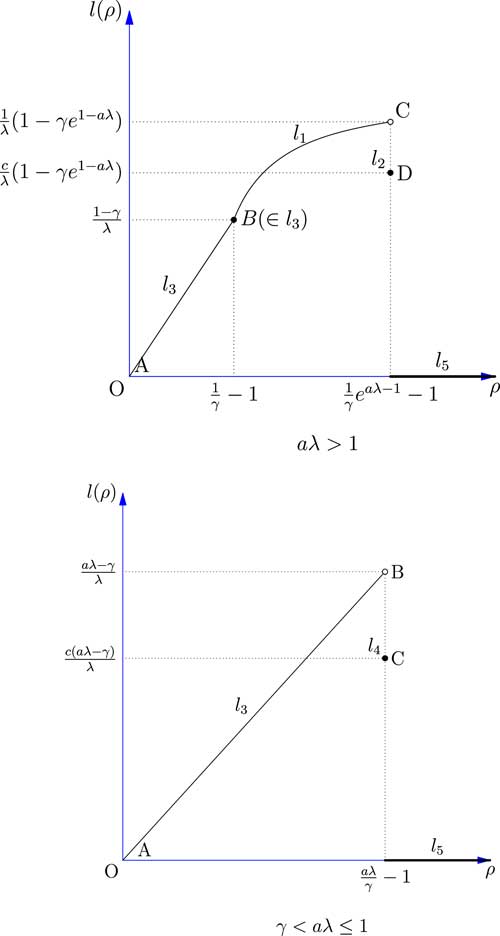
Figure 1 The expected profit of the reinsurer facing one risk.
The results shows that when aλ>1, the optimal expected profit of the reinsurer may not be attainable: as ρ goes to
 $${1 \over \gamma }e^{{a\lambda {\minus}1}} {\minus}1$$
, the expected profit will increase accordingly but may not reach a maximum value. The reason is that in Case 2, the insurer is indifferent to any constant c∈[0, 1], and hence the reinsurer cannot precisely predict which c the insurer will choose. This creates a possible jump between l
1 and l
2 at
$${1 \over \gamma }e^{{a\lambda {\minus}1}} {\minus}1$$
, the expected profit will increase accordingly but may not reach a maximum value. The reason is that in Case 2, the insurer is indifferent to any constant c∈[0, 1], and hence the reinsurer cannot precisely predict which c the insurer will choose. This creates a possible jump between l
1 and l
2 at
 $$\rho \,{\equals}\,{1 \over \gamma }e^{{a\lambda {\minus}1}} {\minus}1$$
.
$$\rho \,{\equals}\,{1 \over \gamma }e^{{a\lambda {\minus}1}} {\minus}1$$
.
When γ<aλ≤1, the optimal expected profit of the reinsurer again may not be obtainable. As ρ goes to
 $${{a\lambda } \over \gamma }{\minus}1$$
, the expected profit of the reinsurer will increase accordingly but there could be a jump between l
3 and l
4 because of the arbitrariness of the constant c in Case 4.
$${{a\lambda } \over \gamma }{\minus}1$$
, the expected profit of the reinsurer will increase accordingly but there could be a jump between l
3 and l
4 because of the arbitrariness of the constant c in Case 4.
2.3.2 Maximising expected utility of the reinsurer
For this optimisation model, we suppose that the utility function of the reinsurer is exponential:
 $$U(x){\equals}\,{\minus}e^{{{\minus}\theta x}} ,\theta \,\gt\,0$$
which is commonly used in financial economics because of its analytical tractability. The analysis works for other utility functions as well, such as linear utility, quadratic utility. An example using the quadratic utility is provided in Appendix B. The profit of the reinsurer is again denoted by A, so that
 $$A{\equals}\,(1{\plus}\rho )\def\Bbb{\tf="Macopen"}\def\Bbb{\tf="Macopen"}{\Bbb E}[f(X)]\,{\minus}\,f(X)$$
We denote the objective function by
 $$k(\rho ){\equals}\,\def\Bbb{\tf="Macopen"}{\Bbb E}[U(A)]$$
The optimisation problem we want to solve in this subsection is the following:
 $$\mathop {{\rm max}}\limits_\rho \,k(\rho ){\equals}\,\mathop {{\rm max}}\limits_\rho \,\def\Bbb{\tf="Macopen"}{\Bbb E}[U(A)]$$
To solve this problem, we apply the results about the value range of the safety loading ρ derived in section 2.2.
Case 1: For aλ>1, we have
 $$\rho \in\big( {{1 \over \gamma }{\minus}1,{1 \over \gamma }e^{{a\lambda {\minus}1}} {\minus}1} \big)$$
and the ceded loss function chosen by the insurer is given by f(x)=(x−d*)+. The profit of the reinsurer hence can be stated as
$$\rho \in\big( {{1 \over \gamma }{\minus}1,{1 \over \gamma }e^{{a\lambda {\minus}1}} {\minus}1} \big)$$
and the ceded loss function chosen by the insurer is given by f(x)=(x−d*)+. The profit of the reinsurer hence can be stated as
 $$A_{1} {\equals}\,(1{\plus}\rho )\def\Bbb{\tf="Macopen"}{\Bbb E}\left[ {X\,{\minus}\,d^{{\asterisk}} } \right]\!_{{\plus}} \,{\minus}\,\left( {X\,{\minus}\,d^{{\asterisk}} } \right)_{\!{\plus}} {\equals}\,{1 \over \lambda }\,{\minus}\,\left( {X\,{\minus}\,d^{{\asterisk}} } \right)_{\!{\plus}} $$
Fact 1.
We introduce a random variable Y given by Y=(X−d*)+, then Y|X>d* follows the exponential distribution with its density function
 $$f_{{\left. Y \right|X\,\gt\,d^{{\asterisk}} }} (y){\equals}\,\lambda e^{{{\minus}\lambda y}} $$
.
$$f_{{\left. Y \right|X\,\gt\,d^{{\asterisk}} }} (y){\equals}\,\lambda e^{{{\minus}\lambda y}} $$
.
We derive the objective function as follows:
 $$\eqalignno{ k_{1} (\rho ){\equals}\, & \def\Bbb{\tf="Macopen"}{\Bbb E}\left[ {U\left( {A_{1} } \right)} \right] \cr {\equals}\, & \left[ {1{\minus}\rho ^{{\asterisk}} } \right]\def\Bbb{\tf="Macopen"}{\Bbb E}\big[ {{\minus}e^{{{\minus}{\theta \over \lambda }}} } \big]{\plus}\rho ^{{\asterisk}} \def\Bbb{\tf="Macopen"}{\Bbb E}\left[ {{\minus}e^{{{\minus}\theta \left[ {{1 \over \lambda }{\minus}\left( {X{\minus}d^{{\asterisk}} } \right)_{{\plus}} } \right]}} \left| {X\,\gt\,d^{{\asterisk}} } \right.} \right] \cr {\equals}\, & \left( {1{\minus}\rho ^{{\asterisk}} } \right)\big( {{\minus}e^{{{\minus}{\theta \over \lambda }}} } \big){\minus}\rho ^{{\asterisk}} \lambda e^{{{\minus}{\theta \over \lambda }}} {\int}_0^\infty e^{{(\theta {\minus}\lambda )y}} dy $$
From this equation, we have the following conclusion:
-
∙ If θ<λ,
$$k_{1} (\rho ){\equals}\,{\minus}e^{{{\minus}{\theta \over \lambda }}} {\plus}{\theta \over {\theta {\minus}\lambda }}e^{{{\minus}{\theta \over \lambda }}} {1 \over {1{\plus}\rho }}$$
. -
∙ Otherwise, if θ≥λ, k 1(ρ)=−∞, which is the worst possible result and hence could be ignored.
When θ<λ, k 1(ρ) is increasing and concave. The value range of k 1(ρ) is given by
 $$k_{1} (\rho )\in\left( {\left( {{{\gamma \theta } \over {\theta {\minus}\lambda }}{\minus}1} \right)e^{{{\minus}{\theta \over \lambda }}} ,{\minus}e^{{{\minus}{\theta \over \lambda }}} {\plus}{{\gamma \theta } \over {\theta \,{\minus}\,\gamma }}e^{{1{\minus}a\lambda {\minus}{\theta \over \lambda }}} } \right)$$
when
 $$\rho \in\big( {{1 \over \gamma }{\minus}1,{1 \over \gamma }e^{{a\lambda {\minus}1}} {\minus}1} \big)$$
. Since the end points of the interval of ρ cannot be achieved, k
1(ρ) will go to its supremum as ρ goes to
$$\rho \in\big( {{1 \over \gamma }{\minus}1,{1 \over \gamma }e^{{a\lambda {\minus}1}} {\minus}1} \big)$$
. Since the end points of the interval of ρ cannot be achieved, k
1(ρ) will go to its supremum as ρ goes to
 $${1 \over \gamma }e^{{a\lambda {\minus}1}} {\minus}1$$
. To sum up
$${1 \over \gamma }e^{{a\lambda {\minus}1}} {\minus}1$$
. To sum up
 $$\mathop {{\rm sup}}\limits_\rho \,k_{1} (\rho ){\equals}\,{\minus}e^{{{\minus}{\theta \over \lambda }}} {\plus}{{\gamma \theta } \over {\theta \,{\minus}\,\gamma }}e^{{1{\minus}a\lambda {\minus}{\theta \over \lambda }}} $$
 $${\rm when}\quad \rho \nearrow{1 \over \gamma }e^{{a\lambda {\minus}1}} {\minus}1$$
Case 2: For aλ>1, we have
 $$\rho \,{\equals}\,{1 \over \lambda }e^{{a\lambda {\minus}1}} {\minus}1$$
and the ceded loss function used in this case is f(x)= c(x−d*)+, c∈[0, 1]. The profit of the reinsurer is denoted by A
2, then A
2=cA
1. The corresponding objective function k
2 can be derived as follows:
$$\rho \,{\equals}\,{1 \over \lambda }e^{{a\lambda {\minus}1}} {\minus}1$$
and the ceded loss function used in this case is f(x)= c(x−d*)+, c∈[0, 1]. The profit of the reinsurer is denoted by A
2, then A
2=cA
1. The corresponding objective function k
2 can be derived as follows:
 $$\eqalignno{ k_{2} (\rho ){\equals}\, & \def\Bbb{\tf="Macopen"}{\Bbb E}\left[ {U\left( {A_{2} } \right)} \right] \cr {\equals}\, & \left( {1{\minus}\rho ^{{\asterisk}} } \right)\big( {{\minus}e^{{{\minus}{{c\theta } \over \lambda }}} } \big){\minus}\rho ^{{\asterisk}} \lambda e^{{{\minus}{{c\theta } \over \lambda }}} {\int}_0^\infty e^{{(c\theta {\minus}\lambda )y}} dy $$
From (14), we have the following conclusion:
-
∙ If cθ<λ,
$$k_{2} (\rho ){\equals}\,{\minus}e^{{{\minus}{{c\theta } \over \lambda }}} {\plus}{{c\theta } \over {c\theta {\minus}\lambda }}e^{{{\minus}{{c\theta } \over \lambda }}} {1 \over {1{\plus}\rho }}$$
. -
∙ Otherwise, if cθ≥λ, k 2(ρ)=−∞, which is the worst possible result and hence could be ignored.

Since in this case the safety loading ρ only have one possible value, we can write down the maximum value k 2(ρ) directly as follows:
 $$\mathop {{\rm max}\,}\limits_\rho k_{2} (\rho ){\equals}\,{\minus}e^{{{\minus}{{c\theta } \over \lambda }}} {\plus}{{c\theta } \over {c\theta \,{\minus}\,\lambda }}e^{{{\minus}{{c\theta } \over \lambda }}} {1 \over {1{\plus}\rho }}$$
 $${\rm at}\quad \rho \,{\equals}\,{1 \over \gamma }e^{{a\lambda {\minus}1}} {\minus}1$$
Now we compare the results in Case 1 and Case 2. Define
 $$q(\theta ){\equals}\,{\minus}e^{{{\minus}{\theta \over \lambda }}} {\plus}{{\gamma \theta } \over {\theta \,{\minus}\,\gamma }}e^{{1{\minus}a\lambda {\minus}{\theta \over \lambda }}} $$
Since θ<λ, we have q(θ) is increasing in θ. Since cθ≤θ, with c∈[0, 1], we find that q(cθ)≤q(θ). Hence we have the following comparison holds:
 $$\mathop {{\rm max}}\limits_\rho \,k_{2} (\rho )\leq \mathop {{\rm sup}}\limits_\rho \,k_{1} (\rho )$$
Case 3: If aλ>1, we have
 $$0\,\lt\,\rho \leq {1 \over \gamma }{\minus}1$$
. If γ<aλ≤1, we have
$$0\,\lt\,\rho \leq {1 \over \gamma }{\minus}1$$
. If γ<aλ≤1, we have
 $$0\,\lt\,\rho \,\lt\,{{a\lambda } \over \gamma }{\minus}1$$
. The ceded loss function used in this case is full insurance f(x)=x. The profit of the reinsurer is denoted by A
3, and we have
$$0\,\lt\,\rho \,\lt\,{{a\lambda } \over \gamma }{\minus}1$$
. The ceded loss function used in this case is full insurance f(x)=x. The profit of the reinsurer is denoted by A
3, and we have
 $$A_{3} {\equals}\,(1{\plus}\rho )\def\Bbb{\tf="Macopen"}{\Bbb E}[X]{\minus}X{\equals}\,(1{\plus}\rho ){\gamma \over \lambda }{\minus}X$$
The objective function can be derived as follows:
 $$\eqalignno{ k_{3} (\rho ){\equals}\, & \def\Bbb{\tf="Macopen"}{\Bbb E}\left[ {U\left( {A_{3} } \right)} \right] \cr & \vskip-5pt{\equals}\,{\minus}\gamma \lambda e^{{{\minus}\theta (1{\plus}\rho ){\gamma \over \lambda }}} {\int}_0^\infty e^{{(\theta {\minus}\lambda )x}} dx $$
We then have the following conclusion by analysing (16):
-
∙ If θ<λ,
$$k_{3} (\rho ){\equals}\,{{\lambda \gamma } \over {\theta {\minus}\lambda }}e^{{{\minus}\theta (1{\plus}\rho ){\gamma \over \lambda }}} $$
. -
∙ Otherwise, if θ≥λ, k 3(ρ)=−∞, which is the worst possible result and hence could be ignored.
So we assume that θ<λ, and it is easy to see that k
3(ρ) is increasing and concave over ρ. Therefore, if aλ>1, the maximum of k
3(ρ) will be achieved at the largest possible safety loading
 $$\rho \,{\equals}\,{1 \over \gamma }{\minus}1$$
, and we have
$$\rho \,{\equals}\,{1 \over \gamma }{\minus}1$$
, and we have
 $$k_{3} (\rho )\in\big( {\left. {{{\gamma \lambda } \over {\theta {\minus}\lambda }}e^{{{\minus}{{\theta \gamma } \over \lambda }}} ,{{\gamma \lambda } \over {\theta {\minus}\lambda }}e^{{{\minus}{\theta \over \lambda }}} } \big]} \right.$$
when
$$k_{3} (\rho )\in\big( {\left. {{{\gamma \lambda } \over {\theta {\minus}\lambda }}e^{{{\minus}{{\theta \gamma } \over \lambda }}} ,{{\gamma \lambda } \over {\theta {\minus}\lambda }}e^{{{\minus}{\theta \over \lambda }}} } \big]} \right.$$
when
 $$\rho \in\big( {\left. {0,{1 \over \gamma }{\minus}1} \big]} \right.$$
. On the other hand, if γ<aλ≤1, k
3(ρ) will go to its supremum as ρ goes to
$$\rho \in\big( {\left. {0,{1 \over \gamma }{\minus}1} \big]} \right.$$
. On the other hand, if γ<aλ≤1, k
3(ρ) will go to its supremum as ρ goes to
 $${{a\lambda } \over \gamma }{\minus}1$$
, and we have
$${{a\lambda } \over \gamma }{\minus}1$$
, and we have
 $$k_{3} (\rho )\in\big( {{{\gamma \lambda } \over {\theta {\minus}\lambda }}e^{{{\minus}{{\theta \gamma } \over \lambda }}} ,{{\gamma \lambda } \over {\theta {\minus}\lambda }}e^{{{\minus}a\theta }} } \big)$$
when
$$k_{3} (\rho )\in\big( {{{\gamma \lambda } \over {\theta {\minus}\lambda }}e^{{{\minus}{{\theta \gamma } \over \lambda }}} ,{{\gamma \lambda } \over {\theta {\minus}\lambda }}e^{{{\minus}a\theta }} } \big)$$
when
 $$\rho \in\big( {0,{{a\lambda } \over \gamma }{\minus}1} \big)$$
. To sum up, we have
$$\rho \in\big( {0,{{a\lambda } \over \gamma }{\minus}1} \big)$$
. To sum up, we have
 $$\mathop {{\rm sup}\,}\limits_\rho k_{3} (\rho )\left\{ {\matrix{ {\equals}\, \hfill & {k_{3} \big( {{1 \over \gamma }{\minus}1} \big){\equals}\,{{\gamma \lambda } \over {\theta \,{\minus}\,\lambda }}e^{{{\minus}{\theta \over \lambda }}} ,\quad a\lambda \,\gt\,1} \hfill \cr {\equals}\, \hfill & {k_{3} \big( {{{a\lambda } \over \gamma }{\minus}1} \big){\equals}\,{{\gamma \lambda } \over {\theta \,{\minus}\,\lambda }}e^{{{\minus}a\theta }} ,\quad \gamma \,\lt\,a\lambda \leq 1} \hfill \cr } } \right.$$
 $${\rm when}\quad \rho \left\{ {\matrix{ {\equals}\, & \hskip-20pt{{1 \over \gamma }{\minus}1,\quad a\lambda \,\gt\,1} \cr \nearrow & {{{a\lambda } \over \gamma }{\minus}1,\quad \gamma \,\lt\,a\lambda \leq 1} \cr } } \right$$
Now we compare the results obtained in Case 1 and Case 3 when aλ>1. We have
 $${{\rm inf}}_\rho k_{1} (\rho ){\equals}\,{{\rm lim}}_{\rho \,\to\,{1 \over \gamma }{\minus}1} k_{1} (\rho ){\equals}\,\left( {{{\gamma \theta } \over {\theta \,{\minus}\,\lambda }}{\minus}1} \right)e^{{{\minus}{\theta \over \lambda }}} $$
and
$${{\rm inf}}_\rho k_{1} (\rho ){\equals}\,{{\rm lim}}_{\rho \,\to\,{1 \over \gamma }{\minus}1} k_{1} (\rho ){\equals}\,\left( {{{\gamma \theta } \over {\theta \,{\minus}\,\lambda }}{\minus}1} \right)e^{{{\minus}{\theta \over \lambda }}} $$
and
 $${{\rm max}}_\rho k_{3} (\rho ){\equals}\,k_{3} \big( {{1 \over \gamma }{\minus}1} \big){\equals}\,{{\gamma \lambda } \over {\theta \,{\minus}\,\lambda }}e^{{{\minus}{\theta \over \lambda }}} $$
. To compare this two values, we have
$${{\rm max}}_\rho k_{3} (\rho ){\equals}\,k_{3} \big( {{1 \over \gamma }{\minus}1} \big){\equals}\,{{\gamma \lambda } \over {\theta \,{\minus}\,\lambda }}e^{{{\minus}{\theta \over \lambda }}} $$
. To compare this two values, we have
 $$\mathop {{\rm inf}\,}\limits_\rho k_{1} (\rho ){\minus}\mathop {{\rm max}\,}\limits_\rho k_{3} (\rho ){\equals}\,(\gamma {\minus}1)e^{{{\minus}{\theta \over \lambda }}} \,\lt\,0$$
Therefore, it is concluded that
 $$\mathop {{\rm inf}\,}\limits_\rho k_{1} (\rho )\,\lt\,\mathop {{\rm max}}\limits_\rho \,k_{3} (\rho )$$
Case 4: For γ<aλ≤1, we have
 $$\rho \,{\equals}\,{{a\lambda } \over \gamma }{\minus}1$$
. The ceded loss function applied in this case should be f(x)=cx, c∈[0, 1]. The profit of the reinsurer is denoted by A
4, and we have A
4=cA
3. The objective function can be derived as follows:
$$\rho \,{\equals}\,{{a\lambda } \over \gamma }{\minus}1$$
. The ceded loss function applied in this case should be f(x)=cx, c∈[0, 1]. The profit of the reinsurer is denoted by A
4, and we have A
4=cA
3. The objective function can be derived as follows:
 $$\eqalignno{ k_{4} (\rho ){\equals}\, & \def\Bbb{\tf="Macopen"}{\Bbb E}\left[ {U\left( {A_{4} } \right)} \right] \cr \vskip-2pt{\equals}\, & \vskip-2pt{\minus}\gamma \lambda e^{{{\minus}c\theta (1{\plus}\rho ){\gamma \over \lambda }}} {\int}_0^\infty e^{{(c\theta {\minus}\lambda )x}} dx $$
Similar to the argument used in Case 3, we have the following conclusion upon analysing (18):
-
∙ If cθ<λ,
$$k_{4} (\rho ){\equals}\,{{\gamma \lambda } \over {c\theta {\minus}\lambda }}e^{{{\minus}c\theta (1{\plus}\rho ){\gamma \over \lambda }}} $$
. -
∙ Otherwise, if cθ≥λ, we have k 4(ρ)=−∞, which is the worst possible result and hence could be ignored.
Since in this case the safety loading ρ only has one possible value, we can write down the maximum value of k 4(ρ) directly as follows:
 $$\mathop {{\rm max}}\limits_\rho \,k_{4} (\rho ){\equals}\,{{\gamma \lambda } \over {c\theta \,{\minus}\,\lambda }}e^{{{\minus}ac\theta }} $$
 $${\rm at}\quad \rho \,{\equals}\,{{a\lambda } \over \gamma }{\minus}1$$
Next we compare the results in Case 3 and Case 4, when γ<aλ≤1. Define
 $$r(\theta )\,{\equals}\,{{\gamma \lambda } \over {\theta \,{\minus}\,\lambda }}e^{{{\minus}a\theta }} $$
Then
 $${{\rm sup}}_\rho k_{3} (\rho ){\equals}\,r(\theta )$$
, and
$${{\rm sup}}_\rho k_{3} (\rho ){\equals}\,r(\theta )$$
, and
 $${\rm max}_{\rho } k_{4} (\rho ){\equals}\,r(c\theta )$$
. As we have assumed that θ<λ, r(θ) is decreasing in θ. Since cθ≤θ, with c∈[0, 1], we find that r(cθ)≥r(θ) . Hence the following comparison holds:
$${\rm max}_{\rho } k_{4} (\rho ){\equals}\,r(c\theta )$$
. As we have assumed that θ<λ, r(θ) is decreasing in θ. Since cθ≤θ, with c∈[0, 1], we find that r(cθ)≥r(θ) . Hence the following comparison holds:
 $$\mathop {{\rm max}}\limits_\rho \,k_{4} (\rho )\geq \mathop {{\rm sup}\,}\limits_\rho k_{3} (\rho )$$
Case 5: For all other cases, the ceded loss function should be f(x)≡0. Consequently, the corresponding objective function k 5(ρ)≡−1, and the maximum value of k 5(ρ) is also −1:
 $$\mathop {{\rm max}}\limits_\rho \,k_{5} (\rho )\,{\equals}\,{\minus}\!1$$
Figure 2 shows the relationship between the safety loading ρ and the objective function k(ρ). The results of all five cases discussed above are combined and compared. Since the comparison between k 1, k 3 and k 5 partly depends on the value of the parameter θ involved in the exponential utility function, we use two black arrows to indicate the uncertain vertical locations of the curves.
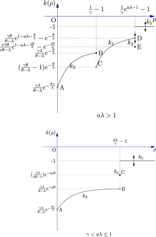
Figure 2 The expected utility of the reinsurer facing one risk.
The results show that if aλ>1, the comparison between point B, point D, and k 5 partly depends on the value of the parameter θ involved in the exponential utility function. So when aλ>1, point D might be lower than point B; point C might be lower than point A; and k 5(ρ) might be lower than point D. Moreover, discontinuity between point D and point E may or may not exist, due to arbitrariness of the constant c in Case 2.
When γ<aλ≤1, k
5(ρ) might be lower than C, in this case the optimal expected exponential utility is obtained in Case 4 and value is
 $${{\gamma \lambda } \over {c\theta \,{\minus}\,\lambda }}e^{{{\minus}ac\theta }} $$
, when ρ is equal to
$${{\gamma \lambda } \over {c\theta \,{\minus}\,\lambda }}e^{{{\minus}ac\theta }} $$
, when ρ is equal to
 $${{a\lambda } \over \gamma }{\minus}1$$
. It should also be remarked that the apparent discontinuity between point B and point C may or may not exist, depending how the insurer chooses the arbitrary constant c in Case 4.
$${{a\lambda } \over \gamma }{\minus}1$$
. It should also be remarked that the apparent discontinuity between point B and point C may or may not exist, depending how the insurer chooses the arbitrary constant c in Case 4.
2.3.3 Minimising VaR of the total loss of the reinsurer
Let Y denote the total loss of the reinsurer, which is given by
 $$Y\,{\equals}\,f(X)\,{\minus}\,\delta _{{f,\rho }} (X)$$
The optimal safety loading problem at confidence level 1−β∈(0, 1) can be stated as
 $$\mathop {{\rm min}}\limits_\rho \:{\rm VaR}\:_{Y} (\beta )$$
Here we assume β≤α because in general the reinsurer’s risk tolerance level is higher. To simplify our notation, we set
 $$b\,\colon\!{\equals}\,S_{X}^{{{\minus}1}} (\beta )$$
. Because of the assumption β≤α, we further have b≥a.
$$b\,\colon\!{\equals}\,S_{X}^{{{\minus}1}} (\beta )$$
. Because of the assumption β≤α, we further have b≥a.
We denote the objective function as j(ρ)=VaR Y (β), and have the following deduction:
 $$\eqalignno{ j(\rho ){\equals}\, & {\rm VaR}_{Y} (\beta ) \cr {\equals}\, & {\rm VaR}_{{f(X)}} (\beta )\,{\minus}\,(1{\plus}\rho )\def\Bbb{\tf="Macopen"}{\Bbb E}[f(X)] \cr {\equals}\, & f[{\rm VaR}\:_{X} (\beta )]\,{\minus}\,(1{\plus}\rho )\def\Bbb{\tf="Macopen"}{\Bbb E}[f(X)] \cr {\equals}\, & f(b)\,{\minus}\,(1{\plus}\rho )\def\Bbb{\tf="Macopen"}{\Bbb E}[f(X)] $$
Here, the second equality comes from the translational invariance of VaR, and the third equality follows from Theorem 1(a) of Dhaene et al. (Reference Dhaene, Denuit, Goovaerts, Kaas and Vyncke2002).
As in previous sections, we assume that X follows a zero-modified exponential distribution with survival function given by
 $$S_{X} (t){\equals}\,\gamma e^{{{\minus}\lambda t}} ,\lambda \,\gt\,0,0\,\lt\,\gamma \,\lt\,1,\:t\,\gt\,0$$
Case 1: For aλ>1, we have
 $$\rho \in\big( {{1 \over \gamma }{\minus}1,{1 \over \gamma }e^{{a\lambda {\minus}1}} {\minus}1} \big)$$
and the ceded loss function is f(x)=(x−d*)+. In this case, our objective function is given by
$$\rho \in\big( {{1 \over \gamma }{\minus}1,{1 \over \gamma }e^{{a\lambda {\minus}1}} {\minus}1} \big)$$
and the ceded loss function is f(x)=(x−d*)+. In this case, our objective function is given by
 $$\eqalignno{ j_{1} (\rho )\,{\equals}\, & f(b){\minus}(1{\plus}\rho )\def\Bbb{\tf="Macopen"}{\Bbb E}[f(X)] \cr {\equals}\, & b{\minus}{1 \over \lambda }{\minus}{1 \over \lambda }{\rm ln}[\gamma (1{\plus}\rho )] $$
Since j
1 is decreasing, j
1(ρ) will go to its infimum as ρ goes to
 $${1 \over \gamma }e^{{a\lambda {\minus}1}} {\minus}1$$
. We can then derive the value range of j
1(ρ):
$${1 \over \gamma }e^{{a\lambda {\minus}1}} {\minus}1$$
. We can then derive the value range of j
1(ρ):
 $$j_{1} (\rho )\in\left( {b{\minus}a,b{\minus}{1 \over \lambda }} \right)$$
when
 $$\rho \in\big( {{1 \over \gamma }{\minus}1,{1 \over \gamma }e^{{a\lambda {\minus}1}} {\minus}1} \big)$$
. Hence we have
$$\rho \in\big( {{1 \over \gamma }{\minus}1,{1 \over \gamma }e^{{a\lambda {\minus}1}} {\minus}1} \big)$$
. Hence we have
 $$\mathop {{\rm inf}}\limits_\rho j_{1} (\rho ){\equals}\,j_{1} \left( {{1 \over \gamma }e^{{a\lambda {\minus}1}} {\minus}1} \right){\equals}\,b{\minus}a$$
 $${\rm when}\quad \rho \nearrow{1 \over \gamma }e^{{a\lambda {\minus}1}} {\minus}1$$
Case 2: If aλ>1, we have
 $$\rho \,{\equals}\,{1 \over \lambda }e^{{a\lambda {\minus}1}} {\minus}1$$
and the ceded loss function is f(x)=c(x−d*)+, c∈[0.1]. Then objective function equals
$$\rho \,{\equals}\,{1 \over \lambda }e^{{a\lambda {\minus}1}} {\minus}1$$
and the ceded loss function is f(x)=c(x−d*)+, c∈[0.1]. Then objective function equals
 $$j_{2} (\rho ){\equals}\,cj_{1} (\rho ){\equals}\,c\left\{ {b{\minus}{1 \over \lambda }{\minus}{1 \over \lambda }{\rm ln}\left[ {\gamma (1{\plus}\rho )} \right]} \right\}$$
In this case, the safety loading ρ only has one possible value, hence we write down the minimum j 2(ρ) as follows:
 $$\mathop {{\rm min}\,}\limits_\rho j_{2} (\rho ){\equals}\,c(b{\minus}a)$$
 $${\rm at}\;\;\rho \,{\equals}\,{1 \over \gamma }e^{{a\lambda {\minus}1}} {\minus}1$$
Now we compare the results derived in Case 1 and Case 2. Since c∈[0, 1], we have c(b−a)≤b−a. Then we have the following comparison holds:
 $$\mathop {{\rm min}}\limits_\rho \,j_{2} (\rho )\leq \mathop {{\rm inf}}\limits_\rho \,j_{1} (\rho )$$
This could be a strict inequality or simply an equality, depending on how the insurer chooses the constant c∈[0, 1].
Case 3: If aλ>1, we have
 $$0\,\lt\,\rho \leq {1 \over \gamma }{\minus}1$$
. Otherwise, if γ<aλ≤1, we have
$$0\,\lt\,\rho \leq {1 \over \gamma }{\minus}1$$
. Otherwise, if γ<aλ≤1, we have
 $$0\,\lt\,\rho \,\lt\,{{a\lambda } \over \gamma }{\minus}1$$
. In this case, the insurer prefers full insurance such that f(x)=x. The corresponding objective function j
3(ρ) in this case is given by
$$0\,\lt\,\rho \,\lt\,{{a\lambda } \over \gamma }{\minus}1$$
. In this case, the insurer prefers full insurance such that f(x)=x. The corresponding objective function j
3(ρ) in this case is given by
 $$\eqalignno{ j_{3} (\rho ){\equals}\, & f(b)\,{\minus}\,(1{\plus}\rho )\def\Bbb{\tf="Macopen"}{\Bbb E}[f(x)] \cr {\equals}\, & b\,{\minus}\,(1{\plus}\rho ){\gamma \over \lambda } $$
Since
 $$j_{3}^{\,'} (\rho ){\equals}\,{\minus}{\gamma \over \lambda }\,\lt\,0$$
, j
3 is decreasing over ρ. If aλ>1, j
3(ρ) will achieve its minimum value at
$$j_{3}^{\,'} (\rho ){\equals}\,{\minus}{\gamma \over \lambda }\,\lt\,0$$
, j
3 is decreasing over ρ. If aλ>1, j
3(ρ) will achieve its minimum value at
 $$\rho \,{\equals}\,{1 \over \gamma }{\minus}1$$
, and we have
$$\rho \,{\equals}\,{1 \over \gamma }{\minus}1$$
, and we have
 $$j_{3} (\rho )\in\left( {\left. {b{\minus}{1 \over \lambda },b{\minus}{\gamma \over \lambda }} \right]} \right.$$
when
$$j_{3} (\rho )\in\left( {\left. {b{\minus}{1 \over \lambda },b{\minus}{\gamma \over \lambda }} \right]} \right.$$
when
 $$\rho \in\big( {\left. {0,{1 \over \gamma }{\minus}1} \big]} \right.$$
. If γ<aλ≤1, j
3(ρ) will go to its infimum as ρ goes to
$$\rho \in\big( {\left. {0,{1 \over \gamma }{\minus}1} \big]} \right.$$
. If γ<aλ≤1, j
3(ρ) will go to its infimum as ρ goes to
 $${{a\lambda } \over \gamma }{\minus}1$$
, and we have
$${{a\lambda } \over \gamma }{\minus}1$$
, and we have
 $$j_{3} (\rho )\in\left( {b{\minus}a,b{\minus}{\gamma \over \lambda }} \right)$$
when
$$j_{3} (\rho )\in\left( {b{\minus}a,b{\minus}{\gamma \over \lambda }} \right)$$
when
 $$\rho \in\big( {0,{{a\lambda } \over \gamma }{\minus}1} \big)$$
. To sum up,
$$\rho \in\big( {0,{{a\lambda } \over \gamma }{\minus}1} \big)$$
. To sum up,
 $$\mathop {{\rm inf}}\limits_\rho \,j_{3} (\rho )\left\{ {\matrix{ {\equals}\, \hfill & {j_{3} \big( {{1 \over \gamma }{\minus}1} \big){\equals}\,b{\minus}{1 \over \lambda },\quad a\lambda \,\gt\,1} \hfill \cr {\equals}\, \hfill & {j_{3} \big( {{{a\lambda } \over \gamma }{\minus}1} \big){\equals}\,b{\minus}a,\quad \gamma \,\lt\,a\lambda \leq 1} \hfill \cr } } \right.$$
 $${\rm when}\quad \rho \left\{ {\matrix{ {\equals}\, \hfill & {{1 \over \gamma }{\minus}1,\quad a\lambda \,\gt\,1} \hfill \cr \nearrow \hfill & {{{a\lambda } \over \gamma }{\minus}1,\quad \gamma \,\lt\,a\lambda \leq 1} \hfill \cr } } \right.$$
Case 4: When aλ≤1, we have
 $$\rho \,{\equals}\,{{a\lambda } \over \gamma }{\minus}1$$
and the ceded loss function is f(x)=cx, c∈[0, 1]. The objective function j
4(ρ) could be derived as follows:
$$\rho \,{\equals}\,{{a\lambda } \over \gamma }{\minus}1$$
and the ceded loss function is f(x)=cx, c∈[0, 1]. The objective function j
4(ρ) could be derived as follows:
 $$\eqalignno{ j_{4} (\rho ){\equals}\, & cj_{3} (\rho ) \cr {\equals}\, & cb\,{\minus}\,c(1{\plus}\rho ){\gamma \over \lambda } $$
As the safety loading ρ can only take on one possible value, we can write down the minimum j 4(ρ) as follows:
 $$\mathop {{\rm min}\,}\limits_\rho j_{4} (\rho ){\equals}\,c(b{\minus}a)$$
 $${\rm at}\quad \rho \,{\equals}\,{{a\lambda } \over \gamma }{\minus}1$$
Now we compare the results derived in Case 3 and Case 4, when γ<aλ≤1. Since c∈[0, 1], we have c(b−a)≤b−a. Then we have the following comparison:
 $$\mathop {{\rm min}\,}\limits_\rho j_{4} (\rho )\leq \mathop {{\rm inf}}\limits_\rho \,j_{3} (\rho )$$
Case 5: For all other cases, the ceded loss function should be identically 0. Consequently, the objective function j 5(ρ)≡0. We can state the result under this circumstance as follows:
 $$\mathop {{\rm max}}\limits_\rho \,j_{5} (\rho ){\equals}\,0$$
Figure 3 shows the relationship between the safety loading ρ and the objective function j(ρ). The results of all five cases discussed above are combined and compared.
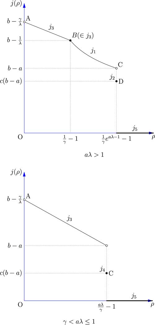
Figure 3 The value-at-risk of the total loss of the reinsurer facing one risk.
The result shows that in both cases aλ>1 and γ<aλ≤1 if we set ρ to be as large as possible, VaR will go to 0 which is optimal. This analysis makes sense in the real insurance and reinsurance markets, because if the reinsurer set its safety loading ρ as large as possible, then the insurer will buy less and less reinsurance for the price is too high. Once the safety loading ρ is larger than some threshold, the insurer will not seek reinsurance at all, and so the ceded loss function f(x) becomes 0. Although the result itself is not too interesting, we will nevertheless demonstrate how it can be applied in some more realistic optimisation problems in section 5.
3 Optimal Safety Loading with Two Risks
3.1 Introduction
When the reinsurer is facing two risks X 1 and X 2 (from insurer 1 and insurer 2), we assume that both insurers are VaR-minimisers: they will apply Theorem 1 to choose the optimal ceded loss function f 1 and f 2, respectively. Since the two insurers might choose different ceded loss functions to cover part of their losses, there will be a total of seven different cases to consider and we need derive the corresponding value range of the safety loading ρ for each case. Three optimisation models: maximising expected profit of the insurer, maximising expected utility of the reinsurer and minimising VaR of the total loss of the reinsurer will be formulated and the optimal safety loading for each model will be derived based on the seven cases.
We suppose the initial losses of the two insurers X 1 and X 2 have unknown dependency structure. We also assume that the two risks X 1 and X 2 follow the same zero-modified exponential distribution:
 $$S_{{X_{i} }} (t){\equals}\,S_{X} (t){\equals}\,\gamma e^{{{\minus}\lambda t}} ,\lambda \,\gt\,0,0\,\lt\,\gamma \,\lt\,1,t\,\gt\,0,i\,{\equals}\,1,2$$
Let α
1 and α
2 be the confidence levels of the two insurers. To simplify the notations, define
 $$a_{1} \,\colon\!{\equals}\,S_{X}^{{{\minus}1}} (\alpha _{1} )$$
and
$$a_{1} \,\colon\!{\equals}\,S_{X}^{{{\minus}1}} (\alpha _{1} )$$
and
 $$a_{2} \,\colon\!{\equals}\,S_{X}^{{{\minus}1}} (\alpha _{2} )$$
. Without loss of generality, we suppose α
1≤α
2, which can derive a
1≥a
2 directly. The reason of assuming the same distribution for both risks is to keep the exposition simple. The method used in the analysis can easily be extended to the situation where X
1 and X
2 have different zero-modified exponential distributions, see Appendix C for an example.
$$a_{2} \,\colon\!{\equals}\,S_{X}^{{{\minus}1}} (\alpha _{2} )$$
. Without loss of generality, we suppose α
1≤α
2, which can derive a
1≥a
2 directly. The reason of assuming the same distribution for both risks is to keep the exposition simple. The method used in the analysis can easily be extended to the situation where X
1 and X
2 have different zero-modified exponential distributions, see Appendix C for an example.
3.2 The value range of the safety loading
Case 1: If both the two insurers would like to choose the stop-loss reinsurance in the form of f(x)=(x−d*)+, we have f 1(x 1)=(x 1−d*)+, f 2(x 2)=(x 2−d*)+. According to Theorem 1 (a), the safety loading ρ has to fulfil the following conditions:
 $$\rho \,\lt\,S_{X} (0)$$
 $$a_{1} \,\gt\,u(\rho ^{{\asterisk}} )$$
 $$a_{2} \,\gt\,u(\rho ^{{\asterisk}} )$$
By applying (1) and (2), we have
 $$\rho \,\lt\,S_{X} (0)\Leftrightarrow\rho \,\gt\,{1 \over \gamma }{\minus}1$$
 $$a_{1} \,\gt\,u(\rho ^{{\asterisk}} )\Leftrightarrow\rho \,\lt\,{1 \over \gamma }e^{{a_{1} \gamma {\minus}1}} {\minus}1$$
 $$a_{2} \,\gt\,u(\rho ^{{\asterisk}} )\Leftrightarrow\rho \,\lt\,{1 \over \gamma }e^{{a_{2} \gamma {\minus}1}} {\minus}1$$
From these results, we obtain
-
∙ If a 2 λ≤1, then ρ does not exist.
-
∙ Otherwise, if a 2 λ>1, we have
$$\rho \in\big( {{1 \over \gamma }{\minus}1,{1 \over \gamma }e^{{a_{2} \lambda {\minus}1}} {\minus}1} \big)$$
.

Hence in this case we will only consider the situation when a 2 λ>1.
Case 2: If both the two insurers would like to choose the change-loss reinsurance in the form of f(x)=c(x−d*)+, c∈[0, 1], we have f 1(x 1)=c(x 1−d*)+, f 2(x 2)=c(x 2−d*)+, c∈[0, 1]. According to Theorem 1 (b), the safety loading ρ has to fulfil the following conditions:
 $$\rho ^{{\asterisk}} \,\lt\,S_{X} (0)$$
 $$a_{1} {\equals}\,a_{2} {\equals}\,u(\rho ^{{\asterisk}} )$$
By applying (3) and (4), we have
 $$\rho ^{{\asterisk}} \,\lt\,S_{X} (0)\Leftrightarrow\rho \,\gt\,{1 \over \gamma }{\minus}1$$
 $$a_{1} {\equals}\,a_{2} {\equals}\,u(\rho ^{{\asterisk}} )\Leftrightarrow\rho \,{\equals}\,{1 \over \gamma }e^{{a_{2} \lambda {\minus}1}} {\minus}1$$
From these results, we have
-
∙ If a 2 λ≤1, ρ does not exist.
-
∙ Otherwise, if a 2 λ>1, we have
$$\rho \,{\equals}\,{1 \over \gamma }e^{{a_{2} \lambda {\minus}1}} {\minus}1$$
.

Hence in this case we will only consider the situation when a 2 λ>1.
Case 3: If both the two insurers would like to choose full reinsurance, then f 1(x 1)=x 1, f 2(x 2)=x 2. According to Theorem 1 (c), the safety loading ρ has to fulfil the following conditions:
 $$\rho ^{{\asterisk}} \geq S_{X} (0)$$
 $$a_{1} \,\gt\,g(0)$$
 $$a_{2} \,\gt\,g(0)$$
From (5) and (6), we have
 $$\rho ^{{\asterisk}} \geq S_{X} (0)\Leftrightarrow\rho \leq {1 \over \gamma }{\minus}1$$
 $$a_{1} \,\gt\,g(0)\Leftrightarrow\rho \,\lt\,{1 \over \gamma }a_{1} \lambda {\minus}1$$
 $$a_{2} \,\gt\,g(0)\Leftrightarrow\rho \,\lt\,{1 \over \gamma }a_{2} \lambda {\minus}1$$
From these results, we conclude that
-
∙ If a 2 λ>1,
$$\rho \in\big( {0\left. {,{1 \over \gamma }{\minus}1} \big]} \right.$$
. -
∙ If γ<a 2 λ≤1,
$$\rho \in\big( {0,{{a_{2} \lambda } \over \gamma }{\minus}1} \big)$$
. -
∙ Otherwise, if a 2 λ≤γ, we have
$$\rho \,\lt\,{{a_{2} \lambda } \over \gamma }{\minus}1\leq 0$$
, which is impossible.


Hence in this case we will only consider the situation when a 2 λ>γ.
Case 4: If both the two insurers would like to choose the quota-share reinsurance in the form of f(x)=cx, c∈[0, 1], we have f 1(x 1)=cx 1, f 2(x 2)=cx 2, c∈[0, 1]. Here, we assume for simplicity that both insurers choose the same constant c. The general case can be dealt with in a similar fashion. According to Theorem 1 (d), the safety loading ρ has to fulfil the following conditions:
 $$\rho ^{{\asterisk}} \geq S_{X} (0)$$
 $$a_{1} {\equals}\,a_{2} {\equals}\,g(0)$$
From (7) and (8), we have
 $$\rho ^{{\asterisk}} \geq S_{X} (0)\Leftrightarrow\rho \leq {1 \over \gamma }{\minus}1$$
 $$a_{1} {\equals}\,a_{2} {\equals}\,g(0)\Leftrightarrow\rho \,{\equals}\,{{a_{2} \lambda } \over \gamma }{\minus}1$$
From these, we may conclude that
-
∙ If a 2 λ>1, ρ does not exist.
-
∙ If γ<a 2 λ≤1, we have
$$\rho \,{\equals}\,{{a_{2} \lambda } \over \gamma }{\minus}1$$
. -
∙ Otherwise, if a 2 λ≤γ, we have
$$\rho \,{\equals}\,{{a_{2} \lambda } \over \gamma }{\minus}1\leq 0$$
, which is impossible.


Hence in this case we only need consider the situation when γ<a 2 λ≤1.
Case 5: Suppose insurer 1 would like to choose the stop-loss reinsurance in the form of f 1(x)= (x−d*)+, and insurer 2 would like to choose the change-loss reinsurance in the form of f 2(x)= c(x−d*)+, c∈[0, 1]. According to Theorem 1 (a) and Theorem 1 (b), the safety loading ρ has to fulfil the following conditions.
 $$\rho ^{{\asterisk}} \,\lt\,S_{X} (0)$$
 $$a_{1} \,\gt\,u(\rho ^{{\asterisk}} )$$
 $$a_{2} {\equals}\,u(\rho ^{{\asterisk}} )$$
By (1), (2) and (4), we have
 $$\rho ^{{\asterisk}} \,\lt\,S_{X} (0)\Leftrightarrow\rho \,\gt\,{1 \over \gamma }{\minus}1$$
 $$a_{1} \,\gt\,u(\rho ^{{\asterisk}} )\Leftrightarrow\rho \,\lt\,{1 \over \gamma }e^{{a_{1} \lambda {\minus}1}} {\minus}1$$
 $$a_{2} {\equals}\,u(\rho ^{{\asterisk}} )\Leftrightarrow\rho \,{\equals}\,{1 \over \gamma }e^{{a_{2} \lambda {\minus}1}} {\minus}1$$
From the results above, we conclude
-
∙ If a 2 λ>1,
$$\rho \,{\equals}\,{1 \over \gamma }e^{{a_{2} \lambda {\minus}1}} {\minus}1$$
. -
∙ Otherwise, ρ does not exist.

Hence in this case we will only consider the situation when a 2 λ>1.
Case 6: Suppose insurer 1 would like to choose full reinsurance in the form of f 1(x)=x, and insurer 2 would like to choose the quota-share reinsurance in the form of f 2(x)=cx, c∈[0, 1]. From Theorem 1 (c) and Theorem 1 (d), the safety loading ρ has to fulfil the following conditions:
 $$\rho ^{{\asterisk}} \geq S_{X} (0)$$
 $$a_{1} \,\gt\,g(0)$$
 $$a_{2} {\equals}\,g(0)$$
From (5), (6) and (8), we obtain
 $$\rho ^{{\asterisk}} \geq S_{X} (0)\Leftrightarrow\rho \leq {1 \over \gamma }{\minus}1$$
 $$a_{1} \,\gt\,g(0)\Leftrightarrow\rho \,\lt\,{{a_{1} \lambda } \over \gamma }{\minus}1$$
 $$a_{2} {\equals}\,g(0)\Leftrightarrow\rho \,{\equals}\,{{a_{2} \lambda } \over \gamma }{\minus}1$$
From these results, we conclude that
-
∙ If γ<a 2 λ≤1,
$$\rho \,{\equals}\,{{a_{2} \lambda } \over \gamma }{\minus}1$$
. -
∙ Otherwise, ρ does not exist.

Hence in this case we only consider the situation when γ<a 2 λ≤1.
Case 7: According to Theorem 1 (e), for all other cases, the optimal ceded loss function is identically 0, so that f 1=f 2≡0.
3.3 Optimisation models
3.3.1 Maximising the expected profit of the reinsurer
The profit of the reinsurer is denoted by
 $$\bar{A},$$
and we have
$$\bar{A},$$
and we have
 $$\bar{A}{\equals}\,(1{\plus}\rho )\def\Bbb{\tf="Macopen"}{\Bbb E}\left( {f_{1} \left( {X_{1} } \right){\plus}f_{2} \left( {X_{2} } \right)} \right){\minus}\left[ {f_{1} \left( {X_{1} } \right){\plus}f_{2} \left( {X_{2} } \right)} \right]$$
The objective function is denoted by
 $$L(\rho ){\equals}\,\def\Bbb{\tf="Macopen"}{\Bbb E}[\bar{A}]\,{\equals}\,\rho \def\Bbb{\tf="Macopen"}{\Bbb E}\left[ {f_{1} \left( {X_{1} } \right){\plus}f_{2} \left( {X_{2} } \right)} \right]$$
Hence the optimal problem can be stated as
 $$\mathop {{\rm max}\,}\limits_\rho L(\rho ){\equals}\,\mathop {{\rm max}\,}\limits_\rho \def\Bbb{\tf="Macopen"}\rho {\Bbb E}\left[ {f_{1} \left( {X_{1} } \right){\plus}f_{2} \left( {X_{2} } \right)} \right]$$
We will apply the results about the value range of the safety loading ρ derived in the previous section to solve this problem.
Case 1: For a
2
λ>1, we have
 $$\rho \in\big( {{1 \over \gamma }{\minus}1,{1 \over \gamma }e^{{a_{2} \lambda {\minus}1}} {\minus}1} \big)$$
. The ceded loss functions for insurer 1 and insurer 2 are f
1(x
1)=(x
1−d*)+ and f
2(x
2)=(x
2−d*)+, respectively. We can derive that
$$\rho \in\big( {{1 \over \gamma }{\minus}1,{1 \over \gamma }e^{{a_{2} \lambda {\minus}1}} {\minus}1} \big)$$
. The ceded loss functions for insurer 1 and insurer 2 are f
1(x
1)=(x
1−d*)+ and f
2(x
2)=(x
2−d*)+, respectively. We can derive that
 $$L_{1} (\rho ){\equals}\,2l_{1} (\rho ){\equals}\,{{2\rho } \over {\lambda (1{\plus}\rho )}}$$
which is increasing and concave over ρ. Hence L
1(ρ) will go to its supremum as ρ goes to
 $${1 \over \gamma }e^{{a_{2} \lambda {\minus}1}} {\minus}1$$
. Since ρ cannot reach
$${1 \over \gamma }e^{{a_{2} \lambda {\minus}1}} {\minus}1$$
. Since ρ cannot reach
 $${1 \over \gamma }e^{{a_{2} \lambda {\minus}1}} {\minus}1$$
, the supremum is not achievable. Moreover, we have
$${1 \over \gamma }e^{{a_{2} \lambda {\minus}1}} {\minus}1$$
, the supremum is not achievable. Moreover, we have
 $$L_{1} (\rho )\in\left( {2\left( {{{1{\minus}\gamma } \over \lambda }} \right),2\left( {{1 \over \lambda }{\minus}{\gamma \over \lambda }e^{{1{\minus}a_{2} \lambda }} } \right)} \right)$$
when
$$L_{1} (\rho )\in\left( {2\left( {{{1{\minus}\gamma } \over \lambda }} \right),2\left( {{1 \over \lambda }{\minus}{\gamma \over \lambda }e^{{1{\minus}a_{2} \lambda }} } \right)} \right)$$
when
 $$\rho \in\big( {{1 \over \gamma }{\minus}1,{1 \over \gamma }e^{{a_{2} \lambda {\minus}1}} {\minus}1} \big)$$
. So we have
$$\rho \in\big( {{1 \over \gamma }{\minus}1,{1 \over \gamma }e^{{a_{2} \lambda {\minus}1}} {\minus}1} \big)$$
. So we have
 $$\mathop {{\rm sup}}\limits_\rho \,L_{1} (\rho ){\equals}\,2\left( {{1 \over \lambda }{\minus}{\gamma \over \lambda }e^{{1{\minus}a_{2} \lambda }} } \right)$$
 $${\rm when}\quad \rho \nearrow{1 \over \gamma }e^{{a_{2} \lambda {\minus}1}} {\minus}1$$
Case 2: For a
2
λ>1, we have
 $$\rho \,{\equals}\,{1 \over \gamma }e^{{a_{2} \lambda {\minus}1}} {\minus}1$$
. The ceded loss functions for insurer 1 and insurer 2 are f
1(x
1)=c(x
1−d*)+ and f
2(x
2)=c(x
2−d*)+, c∈[0, 1], respectively, and we have assumed that the two insurers choose the same constant c for simplicity. We can derive in this case that
$$\rho \,{\equals}\,{1 \over \gamma }e^{{a_{2} \lambda {\minus}1}} {\minus}1$$
. The ceded loss functions for insurer 1 and insurer 2 are f
1(x
1)=c(x
1−d*)+ and f
2(x
2)=c(x
2−d*)+, c∈[0, 1], respectively, and we have assumed that the two insurers choose the same constant c for simplicity. We can derive in this case that
 $$L_{2} (\rho ){\equals}\,2l_{2} (\rho ){\equals}\,{{2c\rho } \over {\lambda (1{\plus}\rho )}}$$
Since the safety loading ρ has only one possible value, so we have
 $$\mathop {{\rm max}}\limits_\rho \,L_{2} (\rho ){\equals}\,2c\left( {{1 \over \lambda }{\minus}{\gamma \over \lambda }e^{{1{\minus}a\lambda }} } \right)$$
 $${\rm at}\quad \rho \,{\equals}\,{1 \over \gamma }e^{{a_{2} \lambda {\minus}1}} {\minus}1$$
We now make a comparison between the results in Case 1 and Case 2 as follows:
 $$\mathop {{\rm max}\,}\limits_\rho L_{2} (\rho )\leq \mathop {{\rm sup}}\limits_\rho \,L_{1} (\rho )$$
Case 3: If a
2
λ>1, we have
 $$\rho \in\big( {\left. {0,{1 \over \gamma }{\minus}1} \big]} \right.$$
. If γ<a
2
λ≤1, we have
$$\rho \in\big( {\left. {0,{1 \over \gamma }{\minus}1} \big]} \right.$$
. If γ<a
2
λ≤1, we have
 $$\rho \in\big( {0,{{a_{2} \lambda } \over \gamma }{\minus}1} \big)$$
. The ceded loss functions for insurer 1 and insurer 2 are f
1(x
1)=x
1 and f
2(x
2)=x
2, respectively. From this, we obtain
$$\rho \in\big( {0,{{a_{2} \lambda } \over \gamma }{\minus}1} \big)$$
. The ceded loss functions for insurer 1 and insurer 2 are f
1(x
1)=x
1 and f
2(x
2)=x
2, respectively. From this, we obtain
 $$L_{3} (\rho ){\equals}\,2l_{3} (\rho ){\equals}\,2{\gamma \over \lambda }\rho $$
which is linear and increasing. Hence if a
2
λ>1, the maximum L
3(ρ) will be achieved at the largest possible safety loading
 $$\rho \,{\equals}\,{1 \over \gamma }{\minus}1$$
, and we have
$$\rho \,{\equals}\,{1 \over \gamma }{\minus}1$$
, and we have
 $$L_{3} (\rho )\in\left( {\left. {0,2\left( {{{1{\minus}\gamma } \over \lambda }} \right)} \right]} \right.$$
when
$$L_{3} (\rho )\in\left( {\left. {0,2\left( {{{1{\minus}\gamma } \over \lambda }} \right)} \right]} \right.$$
when
 $$\rho \in\big( {\left. {0,{1 \over \gamma }{\minus}1} \big]} \right.$$
. On the other hand, if γ<a
2
λ≤1, L
3(ρ) will go to its supremum as ρ goes to
$$\rho \in\big( {\left. {0,{1 \over \gamma }{\minus}1} \big]} \right.$$
. On the other hand, if γ<a
2
λ≤1, L
3(ρ) will go to its supremum as ρ goes to
 $${{a_{2} \lambda } \over \gamma }{\minus}1$$
, and we have
$${{a_{2} \lambda } \over \gamma }{\minus}1$$
, and we have
 $$L_{3} (\rho )\in\left( {0,2\left( {{{a_{2} \lambda {\minus}\gamma } \over \lambda }} \right)} \right)$$
when
$$L_{3} (\rho )\in\left( {0,2\left( {{{a_{2} \lambda {\minus}\gamma } \over \lambda }} \right)} \right)$$
when
 $$\rho \in\big( {0,{{a_{2} \lambda } \over \gamma }{\minus}1} \big)$$
. To sum up
$$\rho \in\big( {0,{{a_{2} \lambda } \over \gamma }{\minus}1} \big)$$
. To sum up
 $$\mathop {{\rm sup}}\limits_\rho \,L_{3} (\rho )\left\{ {\matrix{ {{\equals}\,2\left( {{{1{\minus}\gamma } \over \lambda }} \right),\quad a_{2} \lambda \,\gt\,1} \hfill \cr {{\equals}\,2\left( {{{a_{2} \lambda {\minus}\gamma } \over \lambda }} \right),\quad \gamma \,\lt\,a_{2} \lambda \leq 1} \hfill \cr } } \right.$$
 $${\rm when}\quad \rho \left\{ {\matrix{ {\equals}\, & \hskip-18pt{{1 \over \gamma }{\minus}1,\quad a_{2} \lambda \,\gt\,1} \cr \nearrow & {{{a_{2} \lambda } \over \gamma }{\minus}1,\quad \gamma \,\lt\,a_{2} \lambda \leq 1} \cr } } \right$$
Case 4: For γ<a
2
λ≤1, we have
 $$\rho \,{\equals}\,{{a_{2} \lambda } \over \gamma }{\minus}1$$
. The ceded loss functions for insurer 1 and insurer 2 are f
1(x
1)=cx
1 and f
2(x
2)=cx
2, c∈[0, 1], respectively. Again, we assume that the same c is chosen by the two insurers for simplicity. In this case
$$\rho \,{\equals}\,{{a_{2} \lambda } \over \gamma }{\minus}1$$
. The ceded loss functions for insurer 1 and insurer 2 are f
1(x
1)=cx
1 and f
2(x
2)=cx
2, c∈[0, 1], respectively. Again, we assume that the same c is chosen by the two insurers for simplicity. In this case
 $$L_{4} (\rho ){\equals}\,2l_{4} (\rho ){\equals}\,{{2c\rho \gamma } \over \lambda }$$
Since the safety loading can only be
 $${{a_{2} \lambda } \over \gamma }{\minus}1$$
, we have
$${{a_{2} \lambda } \over \gamma }{\minus}1$$
, we have
 $$\mathop {{\rm max}\,}\limits_\rho L_{4} (\rho ){\equals}\,{{2c(a_{2} \lambda {\minus}\gamma )} \over \lambda }$$
 $${\rm at}\quad \rho \,{\equals}\,{{a_{2} \lambda } \over \gamma }{\minus}1$$
From simple computation, we can compare the optimal values in Case 3 and Case 4 when γ<a 2 λ≤1:
 $$\mathop {{\rm max}}\limits_\rho \,L_{4} (\rho )\leq \mathop {{\rm sup}}\limits_\rho \,L_{3} (\rho )$$
Case 5: For a
2
λ>1, we have
 $$\rho \,{\equals}\,{1 \over \gamma }e^{{a_{2} \lambda {\minus}1}} {\minus}1$$
. The ceded loss functions for insurer 1 and insurer 2 are f
1(x
1)=(x
1−d*)+ and f
2(x
2)=c(x
2−d*)+, c∈[0, 1], respectively, and the corresponding objective function is given by
$$\rho \,{\equals}\,{1 \over \gamma }e^{{a_{2} \lambda {\minus}1}} {\minus}1$$
. The ceded loss functions for insurer 1 and insurer 2 are f
1(x
1)=(x
1−d*)+ and f
2(x
2)=c(x
2−d*)+, c∈[0, 1], respectively, and the corresponding objective function is given by
 $$L_{5} (\rho ){\equals}\,(1{\plus}c)l_{1} (\rho ){\equals}\,{{(1{\plus}c)\rho } \over {\lambda (1{\plus}\rho )}}$$
Since the safety loading ρ can only take on one possible value, so we have
 $$\mathop {{\rm max}}\limits_\rho \,L_{5} (\rho ){\equals}\,(1{\plus}c)\left( {{1 \over \lambda }{\minus}{\gamma \over \lambda }e^{{1{\minus}a_{2} \lambda }} } \right)$$
 $${\rm at}\quad \rho \,{\equals}\,{1 \over \gamma }e^{{a_{2} \lambda {\minus}1}} {\minus}1$$
Now we compare the optimal values in Case 1, Case 2 and Case 5:
 $$\mathop {{\rm max}}\limits_\rho \,L_{2} (\rho )\leq \mathop {{\rm max}}\limits_\rho \,L_{5} (\rho )\leq \mathop {{\rm sup}}\limits_\rho \,L_{1} (\rho )$$
Case 6: For γ<a
2
λ≤1, we have
 $$\rho \,{\equals}\,{{a_{2} \lambda } \over \gamma }{\minus}1$$
. The ceded loss functions for insurer 1 and insurer 2 are f
1(x
1)=x
1 and f
2(x
2)=cx
2, c∈[0, 1], respectively. The objective function is given by
$$\rho \,{\equals}\,{{a_{2} \lambda } \over \gamma }{\minus}1$$
. The ceded loss functions for insurer 1 and insurer 2 are f
1(x
1)=x
1 and f
2(x
2)=cx
2, c∈[0, 1], respectively. The objective function is given by
 $$L_{6} (\rho ){\equals}\,(1{\plus}c)l_{3} (\rho ){\equals}\,(1{\plus}c){\gamma \over \lambda }\rho $$
and we have
 $$\mathop {{\rm max}\,}\limits_\rho L_{6} (\rho ){\equals}\,(1{\plus}c){{a_{2} \lambda {\minus}\gamma } \over \lambda }$$
 $${\rm at}\quad \rho \,{\equals}\,{{a_{2} \lambda } \over \gamma }{\minus}1$$
We can then make comparisons between the results in Case 3, Case 4 and Case 6 when γ<a 2 λ≤1:
 $$\mathop {{\rm max}}\limits_\rho \,L_{4} (\rho )\leq \mathop {{\rm max}}\limits_\rho \,L_{6} (\rho )\leq \mathop {{\rm sup}}\limits_\rho \,L_{3} (\rho )$$
Case 7: For all other cases, f 1=f 2≡0 and thus
 $$\mathop {{\rm max}}\limits_\rho \,L_{7} (\rho ){\equals}\,0$$
Figure 4 shows the relationship between the safety loading ρ and the objective function L(ρ) by combining the results obtained for the seven cases discussed above.
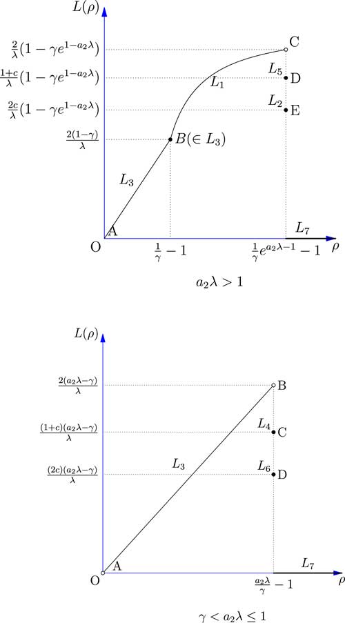
Figure 4 The expected profit of the reinsurer facing two risk.
The results shows that when a
2
λ>1, the optimal expected profit of the reinsurer may not be obtainable, depending on how the constant c is chosen in Case 2 and Case 5. If c is chosen to be 1 in any one of the cases, then point D or point E will coincide with point C, and the maximum expected profit can be achieved at
 $$\rho \,{\equals}\,{1 \over \gamma }e^{{a_{2} \lambda {\minus}1}} {\minus}1$$
. When γ<a
2
λ≤1, the situation is similar. If in either Case 4 or Case 6, c is chosen to be 1, then point C or point D will coincide with point B, and the optimal expected profit of the reinsurer is achieved at
$$\rho \,{\equals}\,{1 \over \gamma }e^{{a_{2} \lambda {\minus}1}} {\minus}1$$
. When γ<a
2
λ≤1, the situation is similar. If in either Case 4 or Case 6, c is chosen to be 1, then point C or point D will coincide with point B, and the optimal expected profit of the reinsurer is achieved at
 $$\rho \,{\equals}\,{{a_{2} \lambda } \over \gamma }{\minus}1$$
.
$$\rho \,{\equals}\,{{a_{2} \lambda } \over \gamma }{\minus}1$$
.
3.3.2 Maximising expected utility of the reinsurer
As in section 3, we assume that the utility function of the reinsurer is given by U(x)=−e
−θx
, θ>0. The profit of the reinsurer is denoted by
 $$\bar{A},$$
and
$$\bar{A},$$
and
 $$\bar{A}{\equals}\,(1{\plus}\rho )\def\Bbb{\tf="Macopen"}{\Bbb E}\left( {f_{1} \left( {X_{1} } \right){\plus}f_{2} \left( {X_{2} } \right)} \right){\minus}\left[ {f_{1} \left( {X_{1} } \right){\plus}f_{2} \left( {X_{2} } \right)} \right]$$
The reinsurer wants to select the optimal ρ so that
 $$K(\rho )\,\,\colon\!{\equals}\,\def\Bbb{\tf="Macopen"}{\Bbb E}[U(\bar{A})]$$
can be maximised:
$$K(\rho )\,\,\colon\!{\equals}\,\def\Bbb{\tf="Macopen"}{\Bbb E}[U(\bar{A})]$$
can be maximised:
 $$\mathop {{\rm max}\,}\limits_\rho K(\rho ){\equals}\,\mathop {{\rm max}}\limits_\rho \,\def\Bbb{\tf="Macopen"}{\Bbb E}[U(\bar{A})]$$
3.3.2.1 Comonotonic Assumption
Suppose that
 $$\big( {\hat{X}_{1} ,\hat{X}_{2} } \big)$$
is a comonotonic copy of (X
1, X
2). As both ceded loss functions f
1 and f
2 are increasing,
$$\big( {\hat{X}_{1} ,\hat{X}_{2} } \big)$$
is a comonotonic copy of (X
1, X
2). As both ceded loss functions f
1 and f
2 are increasing,
 $$\big( {f_{1} \big( {\hat{X}_{1} } \big),f_{2} \big( {\hat{X}_{2} } \big)} \big)$$
is also comonotonic.
$$\big( {f_{1} \big( {\hat{X}_{1} } \big),f_{2} \big( {\hat{X}_{2} } \big)} \big)$$
is also comonotonic.
The following lemma in Dhaene et al. (Reference Dhaene, Denuit, Goovaerts, Kaas and Vyncke2002) indicates that sum of comonotonic random variables is the largest in the sense of convex order.
Lemma 1
Suppose that the random vector
 $$\big( {\hat{X}_{1} ,...,\hat{X}_{n} } \big)\in{\cal F}\big( {F_{1} ,...,F_{n} } \big)$$
is comonotonic, then
$$\big( {\hat{X}_{1} ,...,\hat{X}_{n} } \big)\in{\cal F}\big( {F_{1} ,...,F_{n} } \big)$$
is comonotonic, then
 $$X_{1} {\plus} \cdots {\plus}X_{n} \leq _{{cx}} \hat{X}_{1} {\plus} \cdots {\plus}\hat{X}_{2} $$
for any random vector
 $$\left( {X_{1} ,...,X_{n} } \right)\in{\cal F}\left( {F_{1} ,...,F_{n} } \right)$$
.
$$\left( {X_{1} ,...,X_{n} } \right)\in{\cal F}\left( {F_{1} ,...,F_{n} } \right)$$
.
Then we have
 $$f_{1} \left( {X_{1} } \right){\plus}f_{2} \left( {X_{2} } \right)\leq _{{cx}} f_{1} \big( {\hat{X}_{1} } \big){\plus}f_{2} \big( {\hat{X}_{2} } \big)$$
which implies that
 $$\delta \left( {f_{1} \left( {X_{1} } \right){\plus}f_{2} \left( {X_{2} } \right)} \right){\minus}\left[ {f_{1} \left( {X_{1} } \right){\plus}f_{2} \left( {X_{2} } \right)} \right]\leq _{{cx}} \delta \big( {f_{1} \big( {\hat{X}_{1} } \big){\plus}f\big( {\hat{X}_{2} } \big)} \right){\minus}\left[ {f_{1} \big( {\hat{X}_{1} } \big){\plus}f\big( {\hat{X}_{2} } \big)} \right]$$
Since −U is convex, we have
 $$\def\Bbb{\tf="Macopen"}{\Bbb E}\left[ {U\left( {\delta \left( {f_{1} \left( {X_{1} } \right){\plus}f_{2} \left( {X_{2} } \right)} \right){\minus}\left[ {f_{1} \left( {X_{1} } \right){\plus}f_{2} \left( {X_{2} } \right)} \right]} \right)} \right]\geq \def\Bbb{\tf="Macopen"}{\Bbb E}\left[ {U\left( {\delta \big( {f_{1} \big( {\hat{X}_{1} } \big){\plus}f\big( {\hat{X}_{2} } \big)} \big){\minus}\left[ {f_{1} \big( {\hat{X}_{1} } \big){\plus}f\big( {\hat{X}_{2} } \big)} \right]} \right)} \right]$$
Theorem 2
When
 $$(\hat{X}_{1} ,\hat{X}_{2} )$$
is comonotonic, the expected utility of the profit of the reinsurer would achieve its minimum value. That is
$$(\hat{X}_{1} ,\hat{X}_{2} )$$
is comonotonic, the expected utility of the profit of the reinsurer would achieve its minimum value. That is
 $${\rm max}\,\,{\rm min}\,\def\Bbb{\tf="Macopen"}{\Bbb E}\left[ {U(\bar{A})} \right]{\equals}\,{\rm max}\,\def\Bbb{\tf="Macopen"}{\Bbb E}\left[ {U\left( {\delta \big( {f_{1} \big( {\hat{X}_{1} } \big){\plus}f_{2} \big( {\hat{X}_{2} } \big)} \big){\minus}\left[ {f_{1} \big( {\hat{X}_{1} } \big){\plus}f_{2} \big( {\hat{X}_{2} } \big)} \right]} \right)} \right]$$
where the minimum on the left is taken over all possible dependence structures among X 1 and X 2.
Similar argument for risks under unknown dependency structures can be found in Cheung (Reference Cheung2006). From this theorem, it is reasonable, in view of the unknown dependence structure, to assume that (X 1, X 2) is comonotonic. Now we solve the optimisation problem (23) based on the value ranges of the safety loading ρ derived in section 3.2.
Case 1: For a
2
λ>1, we have
 $$\rho \in\big( {{1 \over \gamma }{\minus}1,{1 \over \gamma }e^{{a_{2} \lambda {\minus}1}} {\minus}1} \big)$$
. The ceded loss functions chosen by insurer 1 and insurer 2 are f
1(x
1)=(x
1−d*)+ and f
2(x
2)=(x
2−d*)+, respectively. The profit of the reinsurer is denoted by
$$\rho \in\big( {{1 \over \gamma }{\minus}1,{1 \over \gamma }e^{{a_{2} \lambda {\minus}1}} {\minus}1} \big)$$
. The ceded loss functions chosen by insurer 1 and insurer 2 are f
1(x
1)=(x
1−d*)+ and f
2(x
2)=(x
2−d*)+, respectively. The profit of the reinsurer is denoted by
 $$\bar{A}_{1} $$
, and we have
$$\bar{A}_{1} $$
, and we have
 $$\bar{A}_{1} {\equals}\,2(1{\plus}\rho )\def\Bbb{\tf="Macopen"}{\Bbb E}\left[ {f_{1} \left( {X_{1} } \right)} \right]{\minus}2f_{1} \left( {X_{1} } \right){\equals}\,2A_{1} $$
Therefore
 $$K_{1} (\rho ){\equals}\,\def\Bbb{\tf="Macopen"}{\Bbb E}\left[ {U\left( {\bar{A}_{1} } \right)} \right]{\equals}\,\def\Bbb{\tf="Macopen"}{\Bbb E}\left[ {U\left( {2A_{1} } \right)} \right]{\equals}\,\def\Bbb{\tf="Macopen"}{\Bbb E}\left[ {{\minus}e^{{{\minus}2\theta A_{1} }} } \right]{\equals}\,{\minus}e^{{{\minus}{{2\theta } \over \lambda }}} {\plus}{{2\theta } \over {2\theta \,{\minus}\,\lambda }}e^{{{\minus}{{2\theta } \over \lambda }}} {1 \over {1{\plus}\rho }}$$
where 2θ<λ, and K 1 is increasing and concave. Moreover
 $$K_{1} (\rho )\in\left( {\left( {{{2\gamma \theta } \over {2\theta \,{\minus}\,\lambda }}{\minus}1} \right)e^{{{\minus}{{2\theta } \over \lambda }}} ,{\minus}e^{{{\minus}{{2\theta } \over \lambda }}} {\plus}{{2\gamma \theta } \over {2\theta {\minus}\gamma }}e^{{1{\minus}a_{2} \lambda {\minus}{{2\theta } \over \lambda }}} } \right)$$
when
 $$\rho \in\big( {{1 \over \gamma }{\minus}1,{1 \over \gamma }e^{{a_{2} \lambda {\minus}1}} {\minus}1} \big)$$
. Since the end points of the interval of ρ are not included, the maximum K
1(ρ) will go to its supremum as ρ goes to
$$\rho \in\big( {{1 \over \gamma }{\minus}1,{1 \over \gamma }e^{{a_{2} \lambda {\minus}1}} {\minus}1} \big)$$
. Since the end points of the interval of ρ are not included, the maximum K
1(ρ) will go to its supremum as ρ goes to
 $${1 \over \gamma }e^{{a_{2} \lambda {\minus}1}} {\minus}1$$
. Therefore, we have
$${1 \over \gamma }e^{{a_{2} \lambda {\minus}1}} {\minus}1$$
. Therefore, we have
 $$\mathop {{\rm sup}}\limits_\rho \,K_{1} (\rho ){\equals}\,{\minus}e^{{{\minus}{{2\theta } \over \lambda }}} {\plus}{{2\theta \gamma } \over {2\theta {\minus}\gamma }}e^{{1{\minus}a_{2} \lambda {\minus}{{2\theta } \over \lambda }}} $$
 $${\rm when}\quad \rho \nearrow{1 \over \gamma }e^{{a_{2} \lambda {\minus}1}} {\minus}1$$
Case 2: For a
2
λ>1, we have
 $$\rho \,{\equals}\,{1 \over \gamma }e^{{a_{2} \lambda {\minus}1}} {\minus}1$$
. The ceded loss functions for insurer 1 and insurer 2 are f
1(x
1)=c(x
1−d*)+ and f
2(x
2)=c(x
2−d*)+, c∈[0, 1], respectively. The profit of the reinsurer is denoted by
$$\rho \,{\equals}\,{1 \over \gamma }e^{{a_{2} \lambda {\minus}1}} {\minus}1$$
. The ceded loss functions for insurer 1 and insurer 2 are f
1(x
1)=c(x
1−d*)+ and f
2(x
2)=c(x
2−d*)+, c∈[0, 1], respectively. The profit of the reinsurer is denoted by
 $$\bar{A}_{2} $$
, and we have
$$\bar{A}_{2} $$
, and we have
 $$\bar{A}_{2} {\equals}\,2A_{2} {\equals}\,2cA_{1} $$
. The objective function is given by
$$\bar{A}_{2} {\equals}\,2A_{2} {\equals}\,2cA_{1} $$
. The objective function is given by
 $$K_{2} (\rho ){\equals}\,\def\Bbb{\tf="Macopen"}{\Bbb E}\left[ {U\left( {2A_{2} } \right)} \right]{\equals}\,\def\Bbb{\tf="Macopen"}{\Bbb E}\left[ {U\left( {2cA_{1} } \right)} \right]{\equals}\,{\minus}e^{{{{{\minus}2c\theta } \over \lambda }}} {\plus}{{2c\theta } \over {2c\theta \,{\minus}\,\lambda }}e^{{{{{\minus}2c\theta } \over \lambda }}} {1 \over {1{\plus}\rho }}$$
where 2cθ<λ. Hence
 $$\mathop {{\rm max}\,}\limits_\rho K_{2} (\rho ){\equals}\,{\minus}e^{{{{{\minus}2c\theta } \over \lambda }}} {\plus}{{2c\theta \gamma } \over {2c\theta \,{\minus}\,\lambda }}e^{{1{\minus}a\lambda {\minus}{{2c\theta } \over \lambda }}} $$
 $${\rm at}\quad \rho \,{\equals}\,{1 \over \gamma }e^{{a_{2} \lambda {\minus}1}} {\minus}1$$
We can make a comparison between the results in Case 1 and Case 2:
 $$\mathop {{\rm max}\,}\limits_\rho K_{2} (\rho )\leq \mathop {{\rm sup}\,}\limits_\rho K_{1} (\rho )$$
Case 3: If a
2
λ>1, we have
 $$\rho \in\big( {\left. {0,{1 \over \gamma }{\minus}1} \big]} \right.$$
. If γ<a
2
λ≤1, we have
$$\rho \in\big( {\left. {0,{1 \over \gamma }{\minus}1} \big]} \right.$$
. If γ<a
2
λ≤1, we have
 $$\rho \in\big( {0,{{a_{2} \lambda } \over \gamma }{\minus}1} \big)$$
. The ceded loss functions for insurer 1 and insurer 2 are f
1(x
1)=x
1 and f
2(x
2)=x
2, respectively. The profit of the reinsurer is denoted by
$$\rho \in\big( {0,{{a_{2} \lambda } \over \gamma }{\minus}1} \big)$$
. The ceded loss functions for insurer 1 and insurer 2 are f
1(x
1)=x
1 and f
2(x
2)=x
2, respectively. The profit of the reinsurer is denoted by
 $$\bar{A}_{3} $$
, and we have
$$\bar{A}_{3} $$
, and we have
 $$\bar{A}_{3} {\equals}\,2A_{3} $$
. By applying the deductions in section 2.3.2, we assume that 2θ<λ and the objective function is given by
$$\bar{A}_{3} {\equals}\,2A_{3} $$
. By applying the deductions in section 2.3.2, we assume that 2θ<λ and the objective function is given by
 $$K_{3} (\rho ){\equals}\,\def\Bbb{\tf="Macopen"}{\Bbb E}\left[ {U\left( {2A_{3} } \right)} \right]{\equals}\,{{\gamma \lambda } \over {2\theta \,{\minus}\,\lambda }}e^{{{\minus}2\theta (1{\plus}\rho ){\gamma \over \lambda }}} $$
It is easy to check that K
3 is increasing and concave in ρ. Therefore if a
2
λ>1, the maximum K
3(ρ) will be achieved at the largest possible safety loading
 $$\rho \,{\equals}\,{1 \over \gamma }{\minus}1$$
, and we have
$$\rho \,{\equals}\,{1 \over \gamma }{\minus}1$$
, and we have
 $$K_{3} (\rho )\in\big( {\left. {{{\gamma \lambda } \over {2\theta \,{\minus}\,\lambda }}e^{{{\minus}{{2\theta \gamma } \over \lambda }}} ,{{\gamma \lambda } \over {2\theta \,{\minus}\,\lambda }}e^{{{\minus}{{2\theta } \over \lambda }}} } \bgi]} \right.$$
when
$$K_{3} (\rho )\in\big( {\left. {{{\gamma \lambda } \over {2\theta \,{\minus}\,\lambda }}e^{{{\minus}{{2\theta \gamma } \over \lambda }}} ,{{\gamma \lambda } \over {2\theta \,{\minus}\,\lambda }}e^{{{\minus}{{2\theta } \over \lambda }}} } \bgi]} \right.$$
when
 $$\rho \in\big( {\left. {0,{1 \over \gamma }{\minus}1} \big]} \right.$$
.
$$\rho \in\big( {\left. {0,{1 \over \gamma }{\minus}1} \big]} \right.$$
.
On the other hand, if γ<a
2
λ≤1, K
3(ρ) will go to its supremum when ρ goes to
 $${{a_{2} \lambda } \over \gamma }{\minus}1$$
, and we have
$${{a_{2} \lambda } \over \gamma }{\minus}1$$
, and we have
 $$K_{3} (\rho )\in\big( {{{\gamma \lambda } \over {2\theta \,{\minus}\,\lambda }}e^{{{\minus}{{2\theta \gamma } \over \lambda }}} ,{{\gamma \lambda } \over {2\theta \,{\minus}\,\lambda }}e^{{{\minus}2a_{2} \theta }} } \big)$$
when
$$K_{3} (\rho )\in\big( {{{\gamma \lambda } \over {2\theta \,{\minus}\,\lambda }}e^{{{\minus}{{2\theta \gamma } \over \lambda }}} ,{{\gamma \lambda } \over {2\theta \,{\minus}\,\lambda }}e^{{{\minus}2a_{2} \theta }} } \big)$$
when
 $$\rho \in\big( {0,{{a_{2} \lambda } \over \gamma }{\minus}1} \big)$$
. To sum up, we obtain:
$$\rho \in\big( {0,{{a_{2} \lambda } \over \gamma }{\minus}1} \big)$$
. To sum up, we obtain:
 $$\mathop {{\rm sup}}\limits_\rho \,K_{3} (\rho )\left\{ {\matrix{ {\equals}\, \hfill & {K_{3} \big( {{1 \over \gamma }{\minus}1} \big){\equals}\,{{\gamma \lambda } \over {2\theta \,{\minus}\,\lambda }}e^{{{\minus}{{2\theta } \over \lambda }}} ,\quad a_{2} \lambda \,\gt\,1} \hfill \cr {\equals}\, \hfill & {K_{3} \big( {{{a_{2} \lambda } \over \gamma }{\minus}1} \big){\equals}\,{{\gamma \lambda } \over {2\theta \,{\minus}\,\lambda }}e^{{{\minus}2a_{2} \theta }} ,\quad \gamma \,\lt\,a_{2} \lambda \leq 1} \hfill \cr } } \right.$$
 $${\rm when}\quad \rho \left\{ {\matrix{ {\equals}\, & \hskip-18pt{{1 \over \gamma }{\minus}1,\quad a_{2} \lambda \,\gt\,1} \cr \nearrow & {{{a_{2} \lambda } \over \gamma }{\minus}1,\quad \gamma \,\lt\,a_{2} \lambda \leq 1} \cr } } \right.$$
To compare the results of Case 1 and Case 3, when a 2 λ>1, we have
 $$\mathop {{\rm inf}}\limits_\rho K_{1} (\rho )\,\lt\,\mathop {{\rm max}}\limits_\rho K_{3} (\rho )$$
Case 4: For γ<a
2
λ≤1, we have
 $$\rho \,{\equals}\,{{a_{2} \lambda } \over \gamma }{\minus}1$$
. The ceded loss functions for insurer 1 and insurer 2 are f
1(x
1)=cx
1 and f
2(x
2)=cx
2, c∈[0, 1]. The profit of the reinsurer is denoted by
$$\rho \,{\equals}\,{{a_{2} \lambda } \over \gamma }{\minus}1$$
. The ceded loss functions for insurer 1 and insurer 2 are f
1(x
1)=cx
1 and f
2(x
2)=cx
2, c∈[0, 1]. The profit of the reinsurer is denoted by
 $$\bar{A}_{4} $$
, and we have
$$\bar{A}_{4} $$
, and we have
 $$\bar{A}_{4} {\equals}\,2A_{4} {\equals}\,2cA_{3} $$
. By applying the deductions in section 2.3.2, we assume that 2cθ<λ, and the objective function is given by
$$\bar{A}_{4} {\equals}\,2A_{4} {\equals}\,2cA_{3} $$
. By applying the deductions in section 2.3.2, we assume that 2cθ<λ, and the objective function is given by
 $$K_{4} (\rho ){\equals}\,\def\Bbb{\tf="Macopen"}{\Bbb E}\left[ {U\left( {2cA_{3} } \right)} \right]{\equals}\,{{\gamma \lambda } \over {2c\theta \,{\minus}\,\lambda }}e^{{{\minus}2\theta (1{\plus}\rho ){\gamma \over \lambda }}} $$
Since in this case the safety loading ρ has only one possible value, we have
 $$\mathop {{\rm max}}\limits_\rho \,K_{4} (\rho ){\equals}\,{{\gamma \lambda } \over {2c\theta \,{\minus}\,\lambda }}e^{{{\minus}2c\theta a_{2} }} $$
 $${\rm at}\quad \rho \,{\equals}\,{{a_{2} \lambda } \over \gamma }{\minus}1$$
We can make a comparison between the results in Case 3 and Case 4 directly by applying (19) when γ<a 2 λ≤1:
 $$\mathop {{\rm max}\,}\limits_\rho K_{4} (\rho )\geq \mathop {{\rm sup}}\limits_\rho \,K_{3} (\rho )$$
Case 5: For a
2
λ>1, we have
 $$\rho \,{\equals}\,{1 \over \gamma }e^{{a_{2} \lambda {\minus}1}} {\minus}1$$
. The ceded loss functions for insurer 1 and insurer 2 are given by f
1(x
1)=(x
1−d*)+ and f
2(x
2)=c(x
2−d*)+, c∈[0, 1], respectively. The profit of the reinsurer is denoted by
$$\rho \,{\equals}\,{1 \over \gamma }e^{{a_{2} \lambda {\minus}1}} {\minus}1$$
. The ceded loss functions for insurer 1 and insurer 2 are given by f
1(x
1)=(x
1−d*)+ and f
2(x
2)=c(x
2−d*)+, c∈[0, 1], respectively. The profit of the reinsurer is denoted by
 $$\bar{A}_{5} $$
, and we have
$$\bar{A}_{5} $$
, and we have
 $$\bar{A}_{5} {\equals}\,(1{\plus}c)A_{1} $$
Using a similar argument, we assume that (1+c)θ<λ and the corresponding objective function is given by
 $$K_{5} (\rho ){\equals}\,{\minus}e^{{{\minus}{{(1{\plus}c)\theta } \over \lambda }}} {\plus}{{(1{\plus}c)\gamma \theta } \over {(1{\plus}c)\theta \,{\minus}\,\lambda }}e^{{{\minus}{{(1{\plus}c)\theta } \over \lambda }}} {1 \over {1{\plus}\rho }}$$
Therefore,
 $$\mathop {{\rm max}}\limits_\rho \,K_{5} (\rho ){\equals}\,{\minus}e^{{{\minus}{{(1{\plus}c)\theta } \over \lambda }}} {\plus}{{(1{\plus}c)\theta \gamma } \over {(1{\plus}c)\theta {\minus}\gamma }}e^{{1{\minus}a_{2} \lambda {\minus}{{(1{\plus}c)\theta } \over \lambda }}} $$
 $${\rm at}\;\;\rho \,{\equals}\,{1 \over \gamma }e^{{a_{2} \lambda {\minus}1}} {\minus}1$$
We can compare the optimal values in Case 1, Case 2 and Case 5 by applying (15):
 $$\mathop {{\rm max}\,}\limits_\rho K_{2} (\rho )\leq \mathop {{\rm max}\,}\limits_\rho K_{5} (\rho )\leq \mathop {{\rm sup}}\limits_\rho \,K_{1} (\rho )$$
Case 6: For a
2
λ≤1, we have
 $$\rho \,{\equals}\,{{a_{2} \lambda } \over \gamma }{\minus}1$$
. The ceded loss functions adopted by insurer 1 and insurer 2 are f
1(x
1)=x
1 and f
2(x
2)=cx
2, c∈[0, 1], respectively. The profit of the reinsurer is denoted by
$$\rho \,{\equals}\,{{a_{2} \lambda } \over \gamma }{\minus}1$$
. The ceded loss functions adopted by insurer 1 and insurer 2 are f
1(x
1)=x
1 and f
2(x
2)=cx
2, c∈[0, 1], respectively. The profit of the reinsurer is denoted by
 $$\bar{A}_{6} $$
, and we have
$$\bar{A}_{6} $$
, and we have
 $$\bar{A}_{6} {\equals}\,(1{\plus}c)A_{3} $$
. With a similar argument used above, we assume that (1+c)θ<λ and the objective function equals
$$\bar{A}_{6} {\equals}\,(1{\plus}c)A_{3} $$
. With a similar argument used above, we assume that (1+c)θ<λ and the objective function equals
 $$K_{6} (\rho ){\equals}\,{{\gamma \lambda } \over {(1{\plus}c)\theta \,{\minus}\,\lambda }}e^{{{\minus}(1{\plus}c)\theta (1{\plus}\rho ){\gamma \over \lambda }}} $$
Moreover, we have
 $$\mathop {{\rm max}\,}\limits_\rho K_{6} (\rho ){\equals}\,{{\gamma \lambda } \over {(1{\plus}c)\theta \,{\minus}\,\lambda }}e^{{{\minus}(1{\plus}c)\theta a_{2} }} $$
 $${\rm at}\quad \rho \,{\equals}\,{{a_{2} \lambda } \over \gamma }{\minus}1$$
We can make comparisons among the results in Case 3, Case 4 and Case 6 by applying (19) when γ<a 2 λ≤1:
 $$\mathop {{\rm max}}\limits_\rho \,K_{4} (\rho )\geq \mathop {{\rm max}}\limits_\rho \,K_{6} (\rho )\geq \mathop {{\rm sup}}\limits_\rho \,K_{3} (\rho )$$
Case 7: For all other cases, the ceded loss functions of the two insurers will be absolutely 0: f 1=f 2≡0. By simple calculation, we obtain
 $$\mathop {{\rm max}\,}\limits_\rho K_{7} (\rho ){\equals}\,{\minus}1$$
Figure 5 shows the relationship between the safety loading ρ and the objective function K(ρ). The results of all seven cases discussed above are combined and compared. Since the comparison between K 1, K 3 and K 7 partly depends on the value of the parameter θ involved in the utility function, we use black arrows to indicate the uncertain vertical locations of the curves.
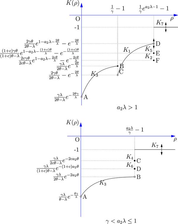
Figure 5 The expected utility of the reinsurer facing two risk.
The results shows that if a
2
λ>1, the comparison between K
1, K
3 and K
7 partly depends on the value of the parameter θ involved in the exponential utility function. So when aλ>1, point D might be lower than point B; point C might be lower than point A; and K
7(ρ) might be lower than point D. When γ<aλ≤1, K
7(ρ) might be lower than point C. Moreover, point E or point F may coincide with point D if the constant c in Case 5 or Case 2 is set at 1. If γ<a
2
λ≤1, the optimal expected exponential utility is obtained either in Case 4 or Case 7, and the reinsurer can always choose
 $$\rho \,{\equals}\,{{a_{2} \lambda } \over \gamma }{\minus}1$$
.
$$\rho \,{\equals}\,{{a_{2} \lambda } \over \gamma }{\minus}1$$
.
3.3.3 Minimising VaR of the total loss of the reinsurer
Following the last subsection, we continue to assume that the losses X 1 and X 2 are comonotonic, despite the fact that VaR is not necessarily subadditive. The comonotonic assumption can simplify many computations involving VaR.
The total loss of the reinsurer is given by
 $$Y\,{\equals}\,f_{1} \left( {X_{1} } \right){\plus}f_{2} \left( {X_{2} } \right){\minus}(1{\plus}\rho )\def\Bbb{\tf="Macopen"}{\Bbb E}\left[ {f_{1} \left( {X_{1} } \right){\plus}f_{2} \left( {X_{2} } \right)} \right]$$
By applying Lemma 6, we get
 $$J(\rho )\,{\equals}\,{\rm VaR}_{Y} (\beta ){\equals}\,f_{1} (b){\plus}f_{2} (b){\minus}(1{\plus}\rho )\def\Bbb{\tf="Macopen"}{\Bbb E}\left[ {f_{1} \left( {X_{1} } \right){\plus}f_{2} \left( {X_{2} } \right)} \right]$$
where β is the confidence level of the reinsurer and we suppose that β≤α 1 and β≤α 2, which implies that b≥a 1 and b≥a 2. The objective of the reinsurer is to minimise J over ρ.
Case 1: For a
2
λ>1, we have
 $$\rho \in\big( {{1 \over \gamma }{\minus}1,{1 \over \gamma }e^{{a_{2} \lambda {\minus}1}} {\minus}1} \big)$$
. The ceded loss functions for insurer 1 and insurer 2 are f
1(x
1)=(x
1−d*)+ and f
2(x
2)=(x
2−d*)+, respectively. By applying the results in (2.3.3), we obtain
$$\rho \in\big( {{1 \over \gamma }{\minus}1,{1 \over \gamma }e^{{a_{2} \lambda {\minus}1}} {\minus}1} \big)$$
. The ceded loss functions for insurer 1 and insurer 2 are f
1(x
1)=(x
1−d*)+ and f
2(x
2)=(x
2−d*)+, respectively. By applying the results in (2.3.3), we obtain
 $$J_{1} (\rho )\,{\equals}\,2j_{1} (\rho )\,{\equals}\,2\left\{ {b{\minus}{1 \over \lambda }{\minus}{1 \over \lambda }\:{\rm ln}\left[ {\gamma (1{\plus}\rho )} \right]} \right\}$$
Since
 $$J_{1}^{\,'} (\rho )\,\lt\,0$$
, J
1 is decreasing over ρ, so J
1(ρ) will go to its infimum when ρ goes to
$$J_{1}^{\,'} (\rho )\,\lt\,0$$
, J
1 is decreasing over ρ, so J
1(ρ) will go to its infimum when ρ goes to
 $${1 \over \gamma }e^{{a_{2} \lambda {\minus}1}} {\minus}1$$
. Moreover, we have
$${1 \over \gamma }e^{{a_{2} \lambda {\minus}1}} {\minus}1$$
. Moreover, we have
 $$J_{1} (\rho )\in\left( {2\left( {b{\minus}a_{2} } \right),2\left( {b{\minus}{1 \over \lambda }} \right)} \right)$$
when
$$J_{1} (\rho )\in\left( {2\left( {b{\minus}a_{2} } \right),2\left( {b{\minus}{1 \over \lambda }} \right)} \right)$$
when
 $$\rho \in\big( {{1 \over \gamma }{\minus}1,{1 \over \gamma }e^{{a_{2} \lambda {\minus}1}} {\minus}1} \big)$$
. Therefore,
$$\rho \in\big( {{1 \over \gamma }{\minus}1,{1 \over \gamma }e^{{a_{2} \lambda {\minus}1}} {\minus}1} \big)$$
. Therefore,
 $$\mathop {{\rm inf}}\limits_\rho \,J_{1} (\rho ){\equals}\,J_{1} \left( {{1 \over \gamma }e^{{a_{2} \lambda {\minus}1}} {\minus}1} \right){\equals}\,2\left( {b{\minus}a_{2} } \right)$$
 $${\rm when}\quad \rho \nearrow{1 \over \gamma }e^{{a_{2} \lambda {\minus}1}} {\minus}1$$
Case 2: For a
2
λ>1, we have
 $$\rho \,{\equals}\,{1 \over \gamma }e^{{a_{2} \lambda {\minus}1}} {\minus}1$$
. The ceded loss functions for two insurers are f
1(x
1)= c(x
1−d*)+, f
2(x
2)=c(x
2−d*)+, c∈[0, 1], where the same c is assumed. By applying results in (2.3.3), we obtain
$$\rho \,{\equals}\,{1 \over \gamma }e^{{a_{2} \lambda {\minus}1}} {\minus}1$$
. The ceded loss functions for two insurers are f
1(x
1)= c(x
1−d*)+, f
2(x
2)=c(x
2−d*)+, c∈[0, 1], where the same c is assumed. By applying results in (2.3.3), we obtain
 $$J_{2} (\rho ){\equals}\,2j_{2} (\rho ){\equals}\,2c\left\{ {b{\minus}{1 \over \lambda }{\minus}{1 \over \lambda }{\rm ln}\left[ {\gamma (1{\plus}\rho )} \right]} \right\}$$
and hence
 $$\mathop {{\rm min}\,}\limits_\rho J_{2} (\rho ){\equals}\,2c\left( {b{\minus}a_{2} } \right)$$
 $${\rm at}\quad \rho \,{\equals}\,{1 \over \gamma }e^{{a_{2} \lambda {\minus}1}} {\minus}1$$
We can make a comparison between the results in Case 1 and Case 2 by applying (20):
 $$\mathop {{\rm min}}\limits_\rho \,J_{2} (\rho )\leq \mathop {{\rm inf}}\limits_\rho \,J_{1} (\rho )$$
Case 3: If a
2
λ>1, we have
 $$\rho \in\big( {\left. {0,{1 \over \gamma }{\minus}1} \big]} \right.$$
. If γ<a
2
λ≤1,
$$\rho \in\big( {\left. {0,{1 \over \gamma }{\minus}1} \big]} \right.$$
. If γ<a
2
λ≤1,
 $$\rho \in\big( {0,{{a_{2} \lambda } \over \gamma }{\minus}1} \big)$$
. The ceded loss functions for insurer 1 and insurer 2 are f
1(x
1)=x
1, f
2(x
2)=x
2, respectively, and we can easily obtain
$$\rho \in\big( {0,{{a_{2} \lambda } \over \gamma }{\minus}1} \big)$$
. The ceded loss functions for insurer 1 and insurer 2 are f
1(x
1)=x
1, f
2(x
2)=x
2, respectively, and we can easily obtain
 $$J_{3} (\rho ){\equals}\,2j_{3} (\rho ){\equals}\,2b{\minus}2(1{\plus}\rho ){\gamma \over \lambda }$$
Since
 $$J_{3}^{'} (\rho )\,\lt\,0$$
, J
3 is decreasing over ρ. If a
2
λ>1, J
3(ρ) will achieve its minimum value at
$$J_{3}^{'} (\rho )\,\lt\,0$$
, J
3 is decreasing over ρ. If a
2
λ>1, J
3(ρ) will achieve its minimum value at
 $$\rho \,{\equals}\,{1 \over \gamma }{\minus}1$$
, and we have
$$\rho \,{\equals}\,{1 \over \gamma }{\minus}1$$
, and we have
 $$J_{3} (\rho )\in\left( {\left. {2b{\minus}{2 \over \lambda },2b{\minus}{{2\gamma } \over \lambda }} \right]} \right.$$
when
$$J_{3} (\rho )\in\left( {\left. {2b{\minus}{2 \over \lambda },2b{\minus}{{2\gamma } \over \lambda }} \right]} \right.$$
when
 $$\rho \in\big( {\left. {0,{1 \over \gamma }{\minus}1} \big]} \right.$$
. If γ<a
2
λ≤1, j
3(ρ) will go to its infimum when ρ goes to
$$\rho \in\big( {\left. {0,{1 \over \gamma }{\minus}1} \big]} \right.$$
. If γ<a
2
λ≤1, j
3(ρ) will go to its infimum when ρ goes to
 $${{a_{2} \lambda } \over \gamma }{\minus}1$$
, and we have
$${{a_{2} \lambda } \over \gamma }{\minus}1$$
, and we have
 $$J_{3} (\rho )\in\left( {2b{\minus}2a_{2} ,2b{\minus}{{2\gamma } \over \lambda }} \right)$$
when
$$J_{3} (\rho )\in\left( {2b{\minus}2a_{2} ,2b{\minus}{{2\gamma } \over \lambda }} \right)$$
when
 $$\rho \in\big( {0,{{a_{2} \lambda } \over \gamma }{\minus}1} \big)$$
. To sum up
$$\rho \in\big( {0,{{a_{2} \lambda } \over \gamma }{\minus}1} \big)$$
. To sum up
 $$\mathop {{\rm inf}}\limits_\rho \,J_{3} (\rho )\left\{ {\matrix{ {\equals}\, \hfill & {J_{3} \big( {{1 \over \gamma }{\minus}1} \big){\equals}\,2b{\minus}{2 \over \lambda },\quad a_{2} \lambda \,\gt\,1} \hfill \cr {\equals}\, \hfill & {J_{3} \big( {{{a_{2} \lambda } \over \gamma }{\minus}1} \big){\equals}\,2b{\minus}2a_{2} ,\quad \gamma \,\lt\,a_{2} \lambda \leq 1} \hfill \cr } } \right.$$
 $${\rm when}\quad \rho \left\{ {\matrix{ {\equals}\, \hfill & {{1 \over \gamma }{\minus}1,\quad a_{2} \lambda \,\gt\,1} \hfill \cr \nearrow \hfill & {{{a_{2} \lambda } \over \gamma }{\minus}1,\quad \gamma \,\lt\,a_{2} \lambda \leq 1} \hfill \cr } } \right.$$
Case 4: For γ<a
2
λ≤1, we have
 $$\rho \,{\equals}\,{{a_{2} \lambda } \over \gamma }{\minus}1$$
. The ceded loss functions for insurer 1 and insurer 2 are given by f
1(x
1)=cx
1, f
2(x
2)=cx
2, c∈[0, 1]. We can derive the objective function as
$$\rho \,{\equals}\,{{a_{2} \lambda } \over \gamma }{\minus}1$$
. The ceded loss functions for insurer 1 and insurer 2 are given by f
1(x
1)=cx
1, f
2(x
2)=cx
2, c∈[0, 1]. We can derive the objective function as
 $$J_{4} (\rho ){\equals}\,2j_{4} (\rho ){\equals}\,2cb{\minus}2c(1{\plus}\rho ){\gamma \over \lambda }$$
and hence
 $$\mathop {{\rm min}\,}\limits_\rho J_{4} (\rho ){\equals}\,2c(b{\minus}a_{2} )$$
 $${\rm at}\quad \rho \,{\equals}\,{{a_{2} \lambda } \over \gamma }{\minus}1$$
We can compare the results in Case 3 and Case 4 by applying ((21)):
 $$\mathop {{\rm min}}\limits_\rho \,J_{4} (\rho )\leq \mathop {{\rm inf}}\limits_\rho \,J_{3} (\rho )$$
Case 5: For a
2
λ>1, we have
 $$\rho \,{\equals}\,{1 \over \gamma }e^{{a_{2} \lambda {\minus}1}} {\minus}1$$
. The ceded loss functions for insurer 1 and insurer 2 are f
1(x
1)=(x
1−d*)+ and f
2(x
2)=c(x
2−d*)+, c∈[0, 1], respectively. Using the same argument, we obtain
$$\rho \,{\equals}\,{1 \over \gamma }e^{{a_{2} \lambda {\minus}1}} {\minus}1$$
. The ceded loss functions for insurer 1 and insurer 2 are f
1(x
1)=(x
1−d*)+ and f
2(x
2)=c(x
2−d*)+, c∈[0, 1], respectively. Using the same argument, we obtain
 $$J_{5} (\rho ){\equals}\,(1{\plus}c)j_{1} (\rho ){\equals}\,(1{\plus}c)\left\{ {b{\minus}{1 \over \lambda }{\minus}{1 \over \lambda }ln\left[ {\gamma (1{\plus}\rho )} \right]} \right\}$$
and thus
 $$\mathop {{\rm min}\,}\limits_\rho J_{5} (\rho ){\equals}\,(1{\plus}c)(b{\minus}a_{2} )$$
 $${\rm at}\;\;\rho \,{\equals}\,{1 \over \gamma }e^{{a_{2} \lambda {\minus}1}} {\minus}1$$
We can also make comparisons among the results in Case 1, Case 2 and Case 5 by applying (20):
 $$\mathop {{\rm min}}\limits_\rho \,J_{2} (\rho )\leq \mathop {{\rm min}}\limits_\rho \,J_{5} (\rho )\leq \mathop {{\rm inf}}\limits_\rho \,J_{1} (\rho )$$
Case 6: For a
2
λ≤1, we have
 $$\rho \,{\equals}\,{{a_{2} \lambda } \over \gamma }{\minus}1$$
. The ceded loss functions for insurer 1 and insurer 2 are f
1(x
1)=x
1 and f
2(x
2)=cx
2, c∈[0, 1], respectively. In this case
$$\rho \,{\equals}\,{{a_{2} \lambda } \over \gamma }{\minus}1$$
. The ceded loss functions for insurer 1 and insurer 2 are f
1(x
1)=x
1 and f
2(x
2)=cx
2, c∈[0, 1], respectively. In this case
 $$J_{6} (\rho ){\equals}\,(1{\plus}c)j_{3} (\rho ){\equals}\,(1{\plus}c)\left[ {b{\minus}(1{\plus}\rho ){\gamma \over \lambda }} \right]$$
which implies that
 $$\mathop {{\rm min}}\limits_\rho \,J_{6} (\rho ){\equals}\,(1{\plus}c)\left( {b{\minus}a_{2} } \right)$$
 $${\rm at}\quad \rho \,{\equals}\,{{a_{2} \lambda } \over \gamma }{\minus}1$$
We can make comparisons among the results in Case 3, Case 4 and Case 6 by using (21):
 $$\mathop {{\rm min}}\limits_\rho \,J_{4} (\rho )\leq \mathop {{\rm min}\,}\limits_\rho J_{6} (\rho )\leq \mathop {{\rm inf}}\limits_\rho \,J_{3} (\rho )$$
Case 7: For all other cases, the ceded loss functions for the two risks will both be exactly 0: f 1=f 2≡0, and hence we have
 $$\mathop {{\rm min}\,}\limits_\rho J_{7} (\rho ){\equals}\,0$$
Figure 6 shows the relationship between the safety loading ρ and the objective function J(ρ). The results of all seven cases discussed above are combined and compared.
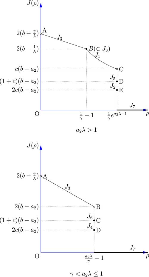
Figure 6 The value-at-risk of the total loss of the reinsurer facing two risk.
Similar with the results for one risk, our results show that in both cases a 2 λ>1 and γ<a 2 λ≤1, if the reinsurer set ρ to be very large, VaR will go to 0 which is optimal. This analysis makes sense in the real reinsurance markets, because if the reinsurer set its safety loading ρ as large as possible, the insurer will purchase less and less reinsurance. Once the safety loading ρ is larger than some threshold, no insurer would buy any reinsurance then the ceded loss function become 0.
4 Applications
Now we illustrate the results derived in the previous sections by using simple numerical examples. Since the results for one risk and for two risks are similar, we will only show examples with one insurer to keep the computation simple.
In section 2.3.2, we derived the optimal safety loading by maximising the expected utility of the reinsurer, the results are not quite certain for comparing the values of the end points in segmented functions. However, if the values of the parameters within the model are given, we could derive the global optimal safety loading (if exists). The following example will give us a clearer picture.
Example 1 (Optimal safety loading by maximising the expected utility of the reinsurer): We would like to solve the optimisation problem stated in section 2.3.2 again with given parameters. The profit of the reinsurer is denoted by A, where
 $$A{\equals}\,(1{\plus}\rho )\def\Bbb{\tf="Macopen"}{\Bbb E}\left[ {f(X)} \right]{\minus}f(X)$$
. We denote the objective function as
$$A{\equals}\,(1{\plus}\rho )\def\Bbb{\tf="Macopen"}{\Bbb E}\left[ {f(X)} \right]{\minus}f(X)$$
. We denote the objective function as
 $$k(\rho ){\equals}\,\def\Bbb{\tf="Macopen"}{\Bbb E}\left[ {U(A)} \right]$$
, and the problem is to
$$k(\rho ){\equals}\,\def\Bbb{\tf="Macopen"}{\Bbb E}\left[ {U(A)} \right]$$
, and the problem is to
 $$\mathop {{\rm max}}\limits_\rho \,k(\rho ){\equals}\,\mathop {{\rm max}}\limits_\rho \,\def\Bbb{\tf="Macopen"}{\Bbb E}\left[ {U(A)} \right]$$
Suppose the initial loss X is zero-modified exponentially distributed: S
X
(t)=γe
−λt
, λ>0, 0<γ<1, t>0. We assume γ=0.5, λ=0.001, so S
X
(t)=0.5e
−0.001t
. The utility function is in the form of U(x)=−e
−θx
,θ>0, and we assume θ=0.0004 so that U(x)=−e
−0.0004x
. The confidence level of the insurer α is assumed to be 0.05, and
 $$a{\equals}\,S_{X}^{{{\minus}1}} (\alpha ){\equals}\,2,302.585$$
. Now we derive the optimal safety loading ρ. There are three forms of reinsurance that the insurer could choose: the stop-loss reinsurance f(x)=(x−d*)+, the change-loss reinsurance f(x)=0.5(x−d*)+, the quota-share reinsurance f(x)=x or f(x)=0.5x.
$$a{\equals}\,S_{X}^{{{\minus}1}} (\alpha ){\equals}\,2,302.585$$
. Now we derive the optimal safety loading ρ. There are three forms of reinsurance that the insurer could choose: the stop-loss reinsurance f(x)=(x−d*)+, the change-loss reinsurance f(x)=0.5(x−d*)+, the quota-share reinsurance f(x)=x or f(x)=0.5x.
In this example we have aλ>1, θ<λ . Following the results derived in section 2.3.2, we can derive the expected utility functions and their maximum or supremum values as follows:
 $$\eqalignno{ 1)\,&k_{1} (\rho )\,{\equals}\,{\minus}e^{{{\minus}{\theta \over \lambda }}} {\plus}{\theta \over {\theta \,{\minus}\,\lambda }}e^{{{\minus}{\theta \over \lambda }}} {1 \over {1{\plus}\rho }}\,{\equals}\,{\minus}0.67032{\minus}{{0.44688} \over {1{\plus}\rho }},\,\rho \in(1,6.3576) \cr & f(x)\,{\equals}\,\left( {x{\minus}d^{{\asterisk}} } \right)_{\!{\plus}} \cr & \mathop{{{\rm sup}}}\limits_{\rho } k_{1} (\rho )\,{\equals}\,k_{1} (6.3576){\equals}\,{\minus}0.6096,\,{\rm when}\,\rho \nearrow6.3576 $$
 $$\hskip-1.8pc\eqalignno{ 2)\,&k_{2} (\rho )\,{\equals}\,{\minus}e^{{{\minus}{{0.5\theta } \over \lambda }}} {\plus}{{0.5\theta } \over {0.5\theta \,{\minus}\,\lambda }}e^{{{\minus}{{0.5\theta } \over \lambda }}} {1 \over {1{\plus}\rho }}\,{\equals}\,{\minus}0.8465,\,\rho \,{\equals}\,6.3576 \cr & f(x)\,{\equals}\,0.5\left( {x{\minus}d^{{\asterisk}} } \right)\!_{{\plus}} \cr & \mathop {{\rm max}}\limits_\rho \,k_{2} (\rho )\,{\equals}\,k_{2} (6.3576)\,{\equals}\,{\minus}0.8465,\,{\rm at}\,\rho \,{\equals}\,6.3576 $$
 $$\hskip-1.8pc\eqalignno{ 3)\,&k_{3} (\rho )\,{\equals}\,{{\lambda \gamma } \over {\theta \,{\minus}\,\lambda }}e^{{{\minus}\theta (1{\plus}\rho ){\gamma \over \lambda }}} \,{\equals}\,{\minus}{5 \over 6}e^{{{\minus}0.2(1{\plus}\rho )}} ,\,\rho \in(0,1] \cr & f(x){\equals}\,x \cr & \mathop {{\rm max}\,}\limits_\rho k_{3} (\rho ){\equals}\,k_{3} (1)\,{\equals}\,{\minus}0.5586,\,{\rm at}\,\rho \,{\equals}\,1 $$
 $$\hskip-4pc\eqalignno{ 4)\,&k_{5} (\rho )\,{\equals}\,{\minus}1,\,\rho \in(6.3576,{\plus}\!\infty) \cr & f(x)\,{\equals}\,0 \cr & \mathop {{\rm max}}\limits_\rho \,k_{5} (\rho )\,{\equals}\,{\minus}1,\,\rho \in(6.3576,{\plus}\!\infty) $$
Therefore, we conclude that the global optimal safety loading ρ is 1, and the maximum expected utility of the reinsurer is −0.5586.
Figure 7 provides us with a whole picture of the results.
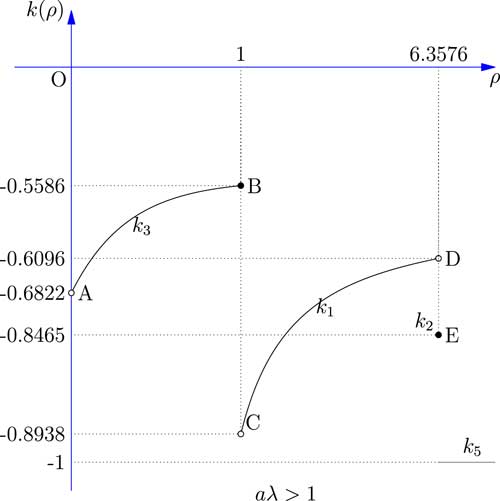
Figure 7 The expected utility of the reinsurer over ρ.This is only a sketch graph which ignores the measures of the coordinates. From the results above we can see that the global optimal safety loading ρ is 1, and the maximum expected utility of the reinsurer will be achieved in point B.
In the real reinsurance market, the safety loading ρ cannot be too big because there are other reinsurers in the market. We suppose the safety loading ρ has an upper bound
 $$\hat{\rho }$$
determined exogenously by the market, so that any safety loading higher than this bound is regarded as completely uncompetitive. We also suppose the reinsurer would like to maximise its utility subject to a VaR constraint, denoted by
$$\hat{\rho }$$
determined exogenously by the market, so that any safety loading higher than this bound is regarded as completely uncompetitive. We also suppose the reinsurer would like to maximise its utility subject to a VaR constraint, denoted by
 $${\rm V{{\vskip -2pt \hskip 2.6pt \hat} \hskip -2.5pt a} }\rm R}$$
. That means the reinsurer would only endure the risk of loss within a certain value.
$${\rm V{{\vskip -2pt \hskip 2.6pt \hat} \hskip -2.5pt a} }\rm R}$$
. That means the reinsurer would only endure the risk of loss within a certain value.
Example 2 The optimisation model is stated as follows:
 $$\eqalignno{ & {\rm max}_{\rho } \def\Bbb{\tf="Macopen"}{\Bbb E}\left[ {U(A)} \right] \cr & s.t{\rm .}\quad {\rm V{a}R}\:_{Y} (\beta )\leq {\rm V \hat a R} \cr & \rho \leq \hat{\rho } $$
We suppose all the information given in Example 1 should also be used in this example. We further suppose the confidence level of the reinsurer β is 0.03, and
 $$b{\equals}\,S_{X}^{{{\minus}1}} (\beta ){\equals}\,2,813.411$$
. We also have
$$b{\equals}\,S_{X}^{{{\minus}1}} (\beta ){\equals}\,2,813.411$$
. We also have
 $$\:{\rm V{\vskip -2pt \hskip 2.6pt \hat} \hskip -2.5pt a}\rm R}$$
=1,800, and
$$\:{\rm V{\vskip -2pt \hskip 2.6pt \hat} \hskip -2.5pt a}\rm R}$$
=1,800, and
 $$\hat{\rho }{\equals}\,2.5$$
. Now we derive the optimal safety loading ρ.
$$\hat{\rho }{\equals}\,2.5$$
. Now we derive the optimal safety loading ρ.
In this example we have aλ>1, θ<λ and
 $$\:{\rm V{{\vskip -2pt \hskip 2.6pt \hat} \hskip -2.5pt a}\rm R}\:\,\lt\,b{\minus}{1 \over \lambda }{\equals}\,1,813.411$$
. Following section 2.3.3, we denote the objective function as j(ρ)=VaR
Y
(β).
$$\:{\rm V{{\vskip -2pt \hskip 2.6pt \hat} \hskip -2.5pt a}\rm R}\:\,\lt\,b{\minus}{1 \over \lambda }{\equals}\,1,813.411$$
. Following section 2.3.3, we denote the objective function as j(ρ)=VaR
Y
(β).
 $${\rm VaR}\:_{Y} (\beta )\leq \:{\rm V{{\vskip -2pt \hskip 2.6pt \hat} \hskip -2.5pt a}\rm R}\:$$
 $$\Rightarrow\rho \geq j_{1}^{{{\minus}1}} (1,800){\equals}\,1.027$$
We illustrate this result in Figure 8.
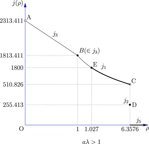
Figure 8 The value-at-risk of the total loss of the reinsurer over ρ. This is only a sketch graph which ignores the measures of the coordinates. The thick lines indicate the possible VaR over ρ.
Then we can restate our optimisation problem as follows:
 $${\rm max}_{\rho } \def\Bbb{\tf="Macopen"}{\Bbb E}\left[ {U(A)} \right]$$
 $${\rm s}{\rm .t}{\rm .}\quad \rho \in[1.027,2.5]$$
The objective function
 $$\def\Bbb{\tf="Macopen"}{\Bbb E}[U(A)]$$
can be denoted as k
1(ρ), where ρ∈[1.027, 2.5]. Since k
1(ρ) is increasing over ρ∈[1.027, 2.5], we have
$$\def\Bbb{\tf="Macopen"}{\Bbb E}[U(A)]$$
can be denoted as k
1(ρ), where ρ∈[1.027, 2.5]. Since k
1(ρ) is increasing over ρ∈[1.027, 2.5], we have
 $${\rm max}_{\rho } \def\Bbb{\tf="Macopen"}{\Bbb E}[U(A)]{\equals}\,k_{1} (2.5){\equals}\,{\minus}0.7979$$
, at ρ=2.5. So the optimal safety loading is 2.5, and the maximum utility of the reinsurer is −0.7979.
$${\rm max}_{\rho } \def\Bbb{\tf="Macopen"}{\Bbb E}[U(A)]{\equals}\,k_{1} (2.5){\equals}\,{\minus}0.7979$$
, at ρ=2.5. So the optimal safety loading is 2.5, and the maximum utility of the reinsurer is −0.7979.
Figure 9 illustrates the results of this example.
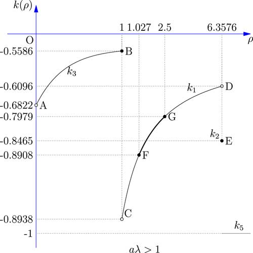
Figure 9 The expected utility of the reinsurer over ρ.
This is only a sketch graph which ignores the measures of the coordinates. The thick line from F to G indicates the possible
 $$\def\Bbb{\tf="Macopen"}{\Bbb E}[U(A)]$$
over ρ, and point G turns out to be the optimal one.
$$\def\Bbb{\tf="Macopen"}{\Bbb E}[U(A)]$$
over ρ, and point G turns out to be the optimal one.
5 Concluding Remarks
In this paper, we considered three optimisation models to study the optimal safety loading that the reinsurer should set. Based on the research done by Cai et al. (Reference Cai, Tan, Weng and Zhang2008), which provided us with the precise form of ceded loss functions chosen by the insurer for any fixed value of safety loading, we solved the problems when the underlying losses are zero-modified exponentially distributed. The three optimisation models from the reinsurer’s perspective are maximising expected profit, maximising expected exponential utility and minimising VaR of the total loss. For the case of two insurers, comonotonicity was assumed because we showed that it is the worst dependency structure in the sense that it gives rise to the lowest expected utility among all possible dependence structures. With the comonotonicity assumption, computation becomes much simpler and tractable.
The results give us inspirations for the reinsurer in choosing its safety loading. In reality, if there are some other constraints, such as the upper bound of the risk tolerance of VaR, we could maximise the expected utility of the reinsurer, it is easy to find the result by applying our conclusions.
However, we could do more exploration in the future to improve this research. First, this research is based on the assumption that the initial loss of the insurer is zero-modified exponentially distributed. This assumption is made because explicit expressions of the optimal safety loadings could be obtained. This assumption could be generalised further, for example, to zero-modified Pareto distribution, see Appendix A. However, explicit expressions of the optimal safety loading cannot be obtained when the assumption of a mixture of exponential distributions is applied. We will explore the possibility to generalise the assumption to the elliptical distributions for further research. Second, although exponential utility is commonly used in financial economics due to its analytical tractability, the use of exponential utility requires that the moment generating function of the loss distribution exists. The assumption of exponential utility used in this paper can be generalised to other utility functions, such as linear utility, quadratic utility. An example using the quadratic utility is provided in Appendix B. Third, we only consider one risk and two risks that the reinsurer might face. It will be interesting if we could generalise the model to n insurers, or a spectrum of insurers described by some measure on an index set. This makes the model closer to the reality. Fourth, We have considered other general risk measures in addition to the VaR risk measure, like distortion risk measures. However, we find that to get closed-form solutions we need to impose specific assumptions on the distortion function, which we are interested in exploring further for further research, along with other possible generalisations. Finally, this research has tried to determine the safety loading by maximising its profit or utility or by minimising its risks. For a real reinsurance company, they might have other considerations to determine their safety loading, which could also be considered in our model in the future.
Acknowledgements
The authors would like to thank the anonymous reviewers for their constructive comments. The authors would also like to thank Dr. K.C. Cheung for his guidance and help in writing the initial version of this paper.
Appendix
A. The Initial Loss of the Insurer Follows a Zero-Modified Pareto Distribution
A.1. Introduction
We assume that the initial loss of the insurer X follows a zero-modified Pareto distribution (Lomax) with survival function
 $$S_{X} {\rm (}t{\rm ) \,{\equals}\, }\gamma \left( {{\theta \over {t{\plus}\theta }}} \right)^{\beta } ,0\,\lt\,\gamma \,\lt\,1,\theta \,\gt\,0,\beta \,\gt\,1$$
Footnote
1
, t>0. Suppose that the reinsurer is facing one risk (one insurer) only. We apply one optimisation criteria from the reinsurer’s point of view as an example to derive the optimal safety loading. The other two optimisation criteria and the case of two insurers discussed in the main text can be derived similarly, which are not shown here.
$$S_{X} {\rm (}t{\rm ) \,{\equals}\, }\gamma \left( {{\theta \over {t{\plus}\theta }}} \right)^{\beta } ,0\,\lt\,\gamma \,\lt\,1,\theta \,\gt\,0,\beta \,\gt\,1$$
Footnote
1
, t>0. Suppose that the reinsurer is facing one risk (one insurer) only. We apply one optimisation criteria from the reinsurer’s point of view as an example to derive the optimal safety loading. The other two optimisation criteria and the case of two insurers discussed in the main text can be derived similarly, which are not shown here.
A.2. The value range of the safety loading
Case 1: If the insurer would like to choose the stop-loss reinsurance in the form of f(x)=(x−d*)+, according to Theorem 1 (a), the safety loading ρ has to fulfil the following two conditions:
-
i. ρ*<S X (0). Then we have
(24)
$${\rm }\rho {\rm \,\gt\,}{1 \over \gamma }{\minus}1$$
-
ii. a>u(ρ*). We have

 $$\rho \,\lt\,{{(a{\plus}\theta )^{\beta } (\beta {\minus}1)^{\beta } } \over {\theta ^{\beta } \beta ^{\beta } \gamma }}{\minus}1$$
From (24) and (25) we have the following conclusion:
-
∙ If
$\big[ {{{(a{\plus}\theta )(\beta {\minus}1)} \over {\theta \beta }}} \big]^{\beta } \leq 1,\rho $
does not exist. -
∙ Otherwise,
$\big[ {{{(a{\plus}\theta )(\beta {\minus}1)} \over {\theta \beta }}} \big]^{\beta } \,\gt\,1$
, we have
$\rho \in\big( {{1 \over \gamma }{\minus}1,{{(a{\plus}\theta )^{\beta } (\beta {\minus}1)^{\beta } } \over {\theta ^{\beta } \beta ^{\beta } \gamma }}{\minus}1} \big)$


So in Case 1 we only need to consider the situation where
 $$\big[ {{{(a{\plus}\theta )(\beta {\minus}1)} \over {\theta \beta }}} \big]^{\beta } \,\gt\,1.$$
Case 2: If the insurer would like to choose the change-loss reinsurance in the form of f(x)= c(x−d*)+ c∈[0, 1], according to Theorem 1 (b), the safety loading ρ has to fulfil the following two conditions:
-
i. ρ*<S X (0) and we have the following result which is the same with that in Case 1
(26)
$$\rho {\vskip -3pt \asterisk}\,\lt\,S_{X} (0)\Leftrightarrow\rho \,\gt\,{1 \over \gamma }{\minus}1$$
-
ii. a=u(ρ*), from which we can derive the value range of ρ as follows by applying the result in Case 1:

 $$\rho {\vskip -3pt \asterisk}\,{\equals}\,{{(a{\plus}\theta )^{\beta } (\beta {\minus}1)^{\beta } } \over {\theta ^{\beta } \beta ^{\beta } \gamma }}{\minus}1$$
From (26) and (27) we obtain the following conclusion:
-
∙ If
$\big[ {{{(a{\plus}\theta )(\beta {\minus}1)} \over {\theta \beta }}} \big]^{\beta } \leq 1,\rho $
does not exist. -
∙ Otherwise,
$\big[ {{{(a{\plus}\theta )(\beta {\minus}1)} \over {\theta \beta }}} \big]^{\beta } \,\gt\,1$
, we have
$\rho {{(a{\plus}\theta )^{\beta } (\beta {\minus}1)^{\beta } } \over {\theta ^{\beta } \beta ^{\beta } \gamma }}{\minus}1$
.

Again, in Case 2 we only need to consider the situation when $\big[ {{{(a{\plus}\theta )(\beta {\minus}1)} \over {\theta \beta }}} \big]^{\beta } \,\gt\,1$
.
$\big[ {{{(a{\plus}\theta )(\beta {\minus}1)} \over {\theta \beta }}} \big]^{\beta } \,\gt\,1$
.
Case 3: If the insurer would like to choose the full reinsurance in the form of f(x)=x, according to Theorem 1 (c), the safety loading ρ has to fulfil the following two conditions:
-
i. ρ*<S X (0), and we have the following deduction:
(28)
$$\rho {\vskip -3pt \asterisk}\geq S_{X} (0)\Leftrightarrow\rho \leq {1 \over \gamma }{\minus}1$$
-
ii. a>g(0), and we have the following deduction:
 $$\rho \,\lt\,{{a(\beta {\minus}1)} \over {\gamma \theta }}{\minus}1$$
Combining (28) and (29), we conclude that
-
∙ If
$${{a(\beta {\minus}1)} \over \theta }\,\gt\,1$$
, we have
$$0\,\lt\,\rho \leq {1 \over \gamma }{\minus}1$$
. -
∙ If
$$\gamma \,\lt\,{{a(\beta {\minus}1)} \over \theta }\leq 1$$
, we have
$$0\,\lt\,\rho \,\lt\,{{a(\beta {\minus}1)} \over {\gamma \theta }}{\minus}1$$
. -
∙ Otherwise
$${{a(\beta {\minus}1)} \over \theta }\leq \gamma $$
, we have
$$\rho \,\lt\,{{a(\beta {\minus}1)} \over {\gamma \theta }}{\minus}1\leq 0$$
, which is impossible.Therefore, in Case 3 we only consider the situation when
$$\gamma \,\lt\,{{a(\beta {\minus}1)} \over \theta }$$
.Case 4: If the insurer would like to choose the quota-share reinsurance in the form of f(x)=cx, c∈[0, 1], according to Theorem 1 (d), the safety loading ρ has to fulfil the following two conditions:
-
i. ρ*≥S X (0). By applying the result derived in Case 3, we have
(30)
$$\rho ^{{\asterisk}} \geq S_{X} (0)\Leftrightarrow\rho \leq {1 \over \gamma }{\minus}1$$
-
ii. a=g(0), and we have the following deduction.
-


 $$a{\equals}\,g(0)\Leftrightarrow\rho \,{\equals}\,{{a(\beta {\minus}1)} \over {\gamma \theta }}{\minus}1$$
From (30) and (31) we have the following results:
-
∙ If
$${{a(\beta {\minus}1)} \over \theta }\,\gt\,1$$
, ρ does not exist. -
∙ If
$$\gamma \,\lt\,{{a(\beta {\minus}1)} \over \theta }\leq 1$$
, we have
$$\rho \,{\equals}\,{{a(\beta {\minus}1)} \over {\gamma \theta }}{\minus}1$$
-
∙ Otherwise
$${{a(\beta {\minus}1)} \over \theta }\leq \gamma $$
, we have
$$\rho \,{\equals}\,{{a(\beta {\minus}1)} \over {\gamma \theta }}{\minus}1\leq 0$$
, which is impossible.


Hence in Case 4 we only consider the situation when
 $$\gamma \,\lt\,{{a(\beta {\minus}1)} \over \theta }\leq 1$$
.
$$\gamma \,\lt\,{{a(\beta {\minus}1)} \over \theta }\leq 1$$
.
Case 5: According to Theorem 1 (e), for all other cases, the optimal ceded loss function is given by f*(x)≡0.
A.3. Maximising the expected profit of the reinsurer
Following the main text, we denote the profit of the reinsurer by A, so that
 $$A{\equals}\,(1{\plus}\rho )\def\Bbb{\tf="Macopen"}{\Bbb E}[f(X)]{\minus}f(X)$$
Then the optimal reinsurance problem can be stated as
 $$\mathop {{\rm max}\,}\limits_\rho l(\rho ){\equals}\,\mathop {{\rm max}}\limits_\rho \,\rho \def\Bbb{\tf="Macopen"}{\Bbb E}[f(X)]$$
We now apply the results about the value range of the safety loading ρ derived in section A.2 and solve the optimisation problem (32) accordingly.
Case 1: For
 $$\big[ {{{(a{\plus}\theta )(\beta {\minus}1)} \over {\theta \beta }}} \right]^{\beta } \,\gt\,1$$
, we have
$$\big[ {{{(a{\plus}\theta )(\beta {\minus}1)} \over {\theta \beta }}} \right]^{\beta } \,\gt\,1$$
, we have
 $$\rho \in\big( {{1 \over \gamma }{\minus}1,{{(a{\plus}\theta )^{\beta } (\beta {\minus}1)^{\beta } } \over {\theta ^{\beta } \beta ^{\beta } \gamma }}{\minus}1} \big)$$
and the ceded loss function should be f(x)=(x−d*)+. We can write the objective function in this case as
$$\rho \in\big( {{1 \over \gamma }{\minus}1,{{(a{\plus}\theta )^{\beta } (\beta {\minus}1)^{\beta } } \over {\theta ^{\beta } \beta ^{\beta } \gamma }}{\minus}1} \big)$$
and the ceded loss function should be f(x)=(x−d*)+. We can write the objective function in this case as
 $$l_{1} (\rho ){\equals}\,\rho \def\Bbb{\tf="Macopen"}{\Bbb E}\left[ {X{\minus}d^{{\asterisk}} } \right]_{\!{\plus}} {\equals}\,{{\gamma ^{{1\,/\,\beta }} \theta } \over {\beta {\minus}1}}\rho (1{\plus}\rho )^{{1\,/\,\beta {\minus}1}} $$
where we can see l
1(ρ) is increasing. Hence l
1(ρ) will go to its supremum value as ρ goes to
 $${{(a{\plus}\theta )^{\beta } (\beta {\minus}1)^{\beta } } \over {\theta ^{\beta } \beta ^{\beta } \gamma }}{\minus}1$$
. Since ρ cannot reach
$${{(a{\plus}\theta )^{\beta } (\beta {\minus}1)^{\beta } } \over {\theta ^{\beta } \beta ^{\beta } \gamma }}{\minus}1$$
. Since ρ cannot reach
 $${{(a{\plus}\theta )^{\beta } (\beta {\minus}1)^{\beta } } \over {\theta ^{\beta } \beta ^{\beta } \gamma }}{\minus}1$$
, the maximum of l
1(ρ) cannot be achieved. Thus
$${{(a{\plus}\theta )^{\beta } (\beta {\minus}1)^{\beta } } \over {\theta ^{\beta } \beta ^{\beta } \gamma }}{\minus}1$$
, the maximum of l
1(ρ) cannot be achieved. Thus
 $$l_{1} (\rho )\in\left( {{{\gamma ^{{1\,/\,\beta }} \theta } \over {\beta {\minus}1}}\big( {{1 \over \gamma }{\minus}1} \big){1 \over \gamma }^{{1\,/\,\beta {\minus}1}} ,{{\gamma ^{{1\,/\,\beta }} \theta } \over {\beta {\minus}1}}\big( {{{(a{\plus}\theta )^{\beta } (\beta {\minus}1)^{\beta } } \over {\theta ^{\beta } \beta ^{\beta } \gamma }}{\minus}1} \big)\big( {{{(a{\plus}\theta )^{\beta } (\beta {\minus}1)^{\beta } } \over {\theta ^{\beta } \beta ^{\beta } \gamma }}} \right)^{{1\,/\,\beta {\minus}1}} } \right)$$
, where
$$l_{1} (\rho )\in\left( {{{\gamma ^{{1\,/\,\beta }} \theta } \over {\beta {\minus}1}}\big( {{1 \over \gamma }{\minus}1} \big){1 \over \gamma }^{{1\,/\,\beta {\minus}1}} ,{{\gamma ^{{1\,/\,\beta }} \theta } \over {\beta {\minus}1}}\big( {{{(a{\plus}\theta )^{\beta } (\beta {\minus}1)^{\beta } } \over {\theta ^{\beta } \beta ^{\beta } \gamma }}{\minus}1} \big)\big( {{{(a{\plus}\theta )^{\beta } (\beta {\minus}1)^{\beta } } \over {\theta ^{\beta } \beta ^{\beta } \gamma }}} \right)^{{1\,/\,\beta {\minus}1}} } \right)$$
, where
 $$\rho \in\big( {{1 \over \gamma }{\minus}1,{{(a{\plus}\theta )^{\beta } (\beta {\minus}1)^{\beta } } \over {\theta ^{\beta } \beta ^{\beta } \gamma }}{\minus}1} \big)$$
. To conclude, we have
$$\rho \in\big( {{1 \over \gamma }{\minus}1,{{(a{\plus}\theta )^{\beta } (\beta {\minus}1)^{\beta } } \over {\theta ^{\beta } \beta ^{\beta } \gamma }}{\minus}1} \big)$$
. To conclude, we have
 $$\mathop {{\rm sup}\,}\limits_\rho l_{1} (\rho ){\equals}\,{{\gamma ^{{1\,/\,\beta }} \theta } \over {\beta {\minus}1}}\left( {{{(a{\plus}\theta )^{\beta } (\beta {\minus}1)^{\beta } } \over {\theta ^{\beta } \beta ^{\beta } \gamma }}{\minus}1} \right)\left( {{{(a{\plus}\theta )^{\beta } (\beta {\minus}1)^{\beta } } \over {\theta ^{\beta } \beta ^{\beta } \gamma }}} \right)^{{1\,/\,\beta {\minus}1}} $$
 $${\rm as}\quad \rho \nearrow{{(a{\plus}\theta )^{\beta } (\beta {\minus}1)^{\beta } } \over {\theta ^{\beta } \beta ^{\beta } \gamma }}{\minus}1$$
Case 2: For
 $$\big[ {{{(a{\plus}\theta )(\beta {\minus}1)} \over {\theta \beta }}} \big]^{\beta } \,\gt\,1$$
, we have
$$\big[ {{{(a{\plus}\theta )(\beta {\minus}1)} \over {\theta \beta }}} \big]^{\beta } \,\gt\,1$$
, we have
 $$\rho \,{\equals}\,{{(a{\plus}\theta )^{\beta } (\beta {\minus}1)^{\beta } } \over {\theta ^{\beta } \beta ^{\beta } \gamma }}{\minus}1$$
and the ceded loss function should be f(x)= c(x−d*)+, c∈[0.1]. We write the objective function in this case as
$$\rho \,{\equals}\,{{(a{\plus}\theta )^{\beta } (\beta {\minus}1)^{\beta } } \over {\theta ^{\beta } \beta ^{\beta } \gamma }}{\minus}1$$
and the ceded loss function should be f(x)= c(x−d*)+, c∈[0.1]. We write the objective function in this case as
 $$l_{2} (\rho ){\equals}\,cl_{1} (\rho ){\equals}\,c{{\gamma ^{{1\,/\,\beta }} \theta } \over {\beta {\minus}1}}\rho (1{\plus}\rho )^{{1\,/\,\beta {\minus}1}} $$
In this case, the safety loading ρ has only one possible value, so we have the maximum l 2(ρ) as follows:
 $$\mathop {{\rm max}\,}\limits_\rho l_{2} (\rho ){\equals}\,{{c\gamma ^{{1\,/\,\beta }} \theta } \over {\beta {\minus}1}}\left( {{{(a{\plus}\theta )^{\beta } (\beta {\minus}1)^{\beta } } \over {\theta ^{\beta } \beta ^{\beta } \gamma }}{\minus}1} \right)\left( {{{(a{\plus}\theta )^{\beta } (\beta {\minus}1)^{\beta } } \over {\theta ^{\beta } \beta ^{\beta } \gamma }}} \right)^{{1\,/\,\beta {\minus}1}} $$
 $${\rm at}\quad \rho \,{\equals}\,{{(a{\plus}\theta )^{\beta } (\beta {\minus}1)^{\beta } } \over {\theta ^{\beta } \beta ^{\beta } \gamma }}{\minus}1$$
Now we compare the supremum or maximum values in Case 1 and Case 2. In both cases we have
 $$\big[ {{{(a{\plus}\theta )(\beta {\minus}1)} \over {\theta \beta }}} \big]^{\beta } \,\gt\,1$$
, and c∈[0, 1], so we obtain that
$$\big[ {{{(a{\plus}\theta )(\beta {\minus}1)} \over {\theta \beta }}} \big]^{\beta } \,\gt\,1$$
, and c∈[0, 1], so we obtain that
 $$\mathop {{\rm max}\,}\limits_\rho l_{2} (\rho )\leq \mathop {{\rm sup}}\limits_\rho \,l_{1} (\rho )$$
Case 3: If
 $${{a(\beta {\minus}1)} \over \theta }\,\gt\,1$$
, we have
$${{a(\beta {\minus}1)} \over \theta }\,\gt\,1$$
, we have
 $$0\,\lt\,\rho \leq {1 \over \gamma }{\minus}1$$
. If
$$0\,\lt\,\rho \leq {1 \over \gamma }{\minus}1$$
. If
 $$\gamma \,\lt\,{{a(\beta {\minus}1)} \over \theta }\leq 1$$
, we have
$$\gamma \,\lt\,{{a(\beta {\minus}1)} \over \theta }\leq 1$$
, we have
 $$0\,\lt\,\rho \,\lt\,{{a(\beta {\minus}1)} \over {\gamma \theta }}{\minus}1$$
. The ceded loss function chosen by the insurer in this case is given by f(x)=x, x≥0. We can write the objective function in this case as
$$0\,\lt\,\rho \,\lt\,{{a(\beta {\minus}1)} \over {\gamma \theta }}{\minus}1$$
. The ceded loss function chosen by the insurer in this case is given by f(x)=x, x≥0. We can write the objective function in this case as
 $$l_{3} (\rho ){\equals}\,\rho \def\Bbb{\tf="Macopen"}{\Bbb E}[X]{\equals}\,{{\rho \gamma \theta } \over {\beta {\minus}1}}$$
which is linear and increasing. If
 $${{a(\beta {\minus}1)} \over \theta }\,\gt\,1$$
, l
3(ρ) achieves its maximum at
$${{a(\beta {\minus}1)} \over \theta }\,\gt\,1$$
, l
3(ρ) achieves its maximum at
 $$\rho \,{\equals}\,{1 \over \gamma }{\minus}1$$
, and we have
$$\rho \,{\equals}\,{1 \over \gamma }{\minus}1$$
, and we have
 $$l_{3} (\rho )\in\big( {\left. {0,{{\theta (1{\minus}\gamma )} \over {\beta {\minus}1}}} \big]} \right.$$
for
$$l_{3} (\rho )\in\big( {\left. {0,{{\theta (1{\minus}\gamma )} \over {\beta {\minus}1}}} \big]} \right.$$
for
 $$\rho \in\big( {\left. {0,{1 \over \gamma }{\minus}1} \big]} \right.$$
. On the other hand, if
$$\rho \in\big( {\left. {0,{1 \over \gamma }{\minus}1} \big]} \right.$$
. On the other hand, if
 $$\gamma \,\lt\,{{a(\beta {\minus}1)} \over \theta }\leq 1$$
, l
3(ρ) will go to its supremum as ρ approaches
$$\gamma \,\lt\,{{a(\beta {\minus}1)} \over \theta }\leq 1$$
, l
3(ρ) will go to its supremum as ρ approaches
 $${{a(\beta {\minus}1)} \over {\gamma \theta }}{\minus}1$$
, and we have
$${{a(\beta {\minus}1)} \over {\gamma \theta }}{\minus}1$$
, and we have
 $$l_{3} (\rho )\in\big( {0,a{\minus}{{\theta \gamma } \over {\beta {\minus}1}}} \big)$$
when
$$l_{3} (\rho )\in\big( {0,a{\minus}{{\theta \gamma } \over {\beta {\minus}1}}} \big)$$
when
 $$\rho \in\big( {0,{{a(\beta {\minus}1)} \over {\gamma \theta }}{\minus}1} \big)$$
. To sum up
$$\rho \in\big( {0,{{a(\beta {\minus}1)} \over {\gamma \theta }}{\minus}1} \big)$$
. To sum up
 $$\mathop {{\rm sup}\,}\limits_\rho l_{3} (\rho )\left\{ {\matrix{ {\equals}\, \hfill & {{{\theta (1{\minus}\gamma )} \over {\beta {\minus}1}},\quad {{a(\beta {\minus}1)} \over \theta }\,\gt\,1} \hfill \cr {\equals}\, \hfill & {a{\minus}{{\theta \gamma } \over {\beta {\minus}1}},\quad \gamma \,\lt\,{{a(\beta {\minus}1)} \over \theta }\leq 1} \hfill \cr } } \right.$$
 $${\rm when}\quad \rho \left\{ {\matrix{ {\equals}\, \hfill & {{1 \over \gamma }{\minus}1,\quad {{a(\beta {\minus}1)} \over \theta }\,\gt\,1} \hfill \cr \nearrow \hfill & {{{a(\beta {\minus}1)} \over {\gamma \theta }}{\minus}1,\quad \gamma \,\lt\,{{a(\beta {\minus}1)} \over \theta }\leq 1} \hfill \cr } } \right.$$
Case 4: For
 $$\gamma \,\lt\,{{a(\beta {\minus}1)} \over \theta }\leq 1$$
, we have the safety loading
$$\gamma \,\lt\,{{a(\beta {\minus}1)} \over \theta }\leq 1$$
, we have the safety loading
 $$\rho \,{\equals}\,{{a(\beta {\minus}1)} \over {\gamma \theta }}{\minus}1$$
. The ceded loss function used in this case should be in the form of f(x)=cx, c∈[0, 1]. We denote the objective function in this case by
$$\rho \,{\equals}\,{{a(\beta {\minus}1)} \over {\gamma \theta }}{\minus}1$$
. The ceded loss function used in this case should be in the form of f(x)=cx, c∈[0, 1]. We denote the objective function in this case by
 $$l_{4} (\rho ){\equals}\,cl_{3} (\rho ){\equals}\,{{c\rho \gamma \theta } \over {\beta {\minus}1}}$$
Since the safety loading can only equal
 $${{a(\beta {\minus}1)} \over {\gamma \theta }}{\minus}1$$
, we have
$${{a(\beta {\minus}1)} \over {\gamma \theta }}{\minus}1$$
, we have
 $$\mathop {{\rm max}\,}\limits_\rho l_{4} (\rho ){\equals}\,ac{\minus}{{c\theta \gamma } \over {\beta {\minus}1}}$$
 $${\rm at}\quad \rho \,{\equals}\,{{a(\beta {\minus}1)} \over {\gamma \theta }}{\minus}1$$
Now we compare the results derived in Case 3 and Case 4 when
 $$\gamma \,\lt\,{{a(\beta {\minus}1)} \over \theta }\leq 1$$
. Since c∈[0, 1], we have
$$\gamma \,\lt\,{{a(\beta {\minus}1)} \over \theta }\leq 1$$
. Since c∈[0, 1], we have
 $$\mathop {{\rm max}}\limits_\rho l_{4} (\rho )\leq \mathop {{\rm sup}}\limits_\rho l_{3} (\rho )$$
Case 5: For other cases, the ceded loss function should be f(x)≡0. Consequently, the corresponding objective function l 5(ρ)≡0, and hence the maximum value of l 5(ρ) will also be 0:
 $$\mathop {{\rm max}\,}\limits_\rho l_{5} (\rho ){\,\equals\,}\,0$$
 $${\rm for}\,{\rm all}\,{\rm other}\,\rho $$
B. Assume the Utility Function of the Reinsurer is Quadratic
For this optimisation model, we suppose that the utility function of the reinsurer is quadratic:
 $$U(x){\equals}\,{\minus}(c{\minus}x)^{2} ,\,x\leq c$$
The profit of the reinsurer is again denoted by A, so that
 $$A{\,\equals\,}\,(1{\plus}\rho )\def\Bbb{\tf="Macopen"}{\Bbb E}[f(X)]{\minus}f(X)$$
We denote the objective function by
 $$k(\rho ){\,\equals\,}\,\def\Bbb{\tf="Macopen"}{\Bbb E}[U(A)]$$
The optimisation problem we want to solve in this subsection is the following:
 $$\mathop {{\rm max}}\limits_\rho \,k(\rho ){\,\equals\,}\,\mathop {{\rm max}}\limits_\rho \,\def\Bbb{\tf="Macopen"}{\Bbb E}[U(A)]$$
To solve this problem, we apply the results about the value range of the safety loading ρ derived in section 2.2.
Case 1: For aλ>1, we have
 $$\rho \in\big( {{1 \over \gamma }{\minus}1,{1 \over \gamma }e^{{a\lambda {\minus}1}} {\minus}1} \big)$$
and the ceded loss function chosen by the insurer is given by f(x)=(x−d*)+. The profit of the reinsurer hence can be stated as
$$\rho \in\big( {{1 \over \gamma }{\minus}1,{1 \over \gamma }e^{{a\lambda {\minus}1}} {\minus}1} \big)$$
and the ceded loss function chosen by the insurer is given by f(x)=(x−d*)+. The profit of the reinsurer hence can be stated as
 $$A_{1} {\equals}\,(1{\plus}\rho )\def\Bbb{\tf="Macopen"}{\Bbb E}\left[ {X{\minus}d^{{\asterisk}} } \right]_{\!{\plus}} {\minus}\left( {X{\minus}d^{{\asterisk}} } \right)\!_{{\plus}} {\equals}\,{1 \over \lambda }{\minus}\left( {X{\minus}d^{{\asterisk}} } \right)_{\!{\plus}} $$
We derive the objective function as follows:
 $$\eqalignno{ k_{1} (\rho ){\equals}\, & \def\Bbb{\tf="Macopen"}{\Bbb E}\left[ {U(A_{1} )} \right] \cr {\equals}\, & \left[ {1{\minus}S_{X} \left( {d^{{\asterisk}} } \right)} \right]\def\Bbb{\tf="Macopen"}{\Bbb E}\left[ {{\minus}\left( {c{\minus}{1 \over \lambda }} \right)^{2} } \right]{\plus}S_{X} \left( {d^{{\asterisk}} } \right)\def\Bbb{\tf="Macopen"}{\Bbb E}\left[ {{\minus}\left( {c{\minus}{1 \over \lambda }{\plus}\left( {X{\minus}d^{{\asterisk}} } \right)_{{\plus}} } \right)^{2} \left| {X\,\gt\,d} \right.^{{\asterisk}} } \right] $$
Using Fact 1 in the main text, we introduce a random variable Y given by Y=(X−d*)+, then Y|X>d* follows the exponential distribution with its density function
 $$f_{{\left. Y \right|X\,\gt\,d^{{\asterisk}} }} (y){\equals}\,\lambda e^{{{\minus}\lambda y}} $$
.
$$f_{{\left. Y \right|X\,\gt\,d^{{\asterisk}} }} (y){\equals}\,\lambda e^{{{\minus}\lambda y}} $$
.
Hence we derive
 $$k_{1} (\rho ){\equals}\,{\minus}\left( {c{\minus}{1 \over \lambda }} \right)^{2} {\minus}{{2c} \over {\lambda (1{\plus}\rho )}}$$
We can see that k 1(ρ) is increasing and concave with respect to ρ. The value range of k 1(ρ) is given by
 $$k_{1} (\rho )\in\left( {{\minus}\left( {c{\minus}{1 \over \lambda }} \right)^{2} {\minus}{{2c\gamma } \over \lambda },{\minus}\left( {c{\minus}{1 \over \lambda }} \right)^{2} {\minus}{{2c\gamma } \over {\lambda e^{{a\lambda {\minus}1}} }}} \right)$$
when
 $$\rho \in\big( {{1 \over \gamma }{\minus}1,{1 \over \gamma }e^{{a\lambda {\minus}1}} {\minus}1} \big)$$
. Since the end points of the interval of ρ cannot be achieved, k
1(ρ) will go to its supremum as ρ goes to
$$\rho \in\big( {{1 \over \gamma }{\minus}1,{1 \over \gamma }e^{{a\lambda {\minus}1}} {\minus}1} \big)$$
. Since the end points of the interval of ρ cannot be achieved, k
1(ρ) will go to its supremum as ρ goes to
 $${1 \over \gamma }e^{{a\lambda {\minus}1}} {\minus}1$$
. To sum up
$${1 \over \gamma }e^{{a\lambda {\minus}1}} {\minus}1$$
. To sum up
 $$\mathop {{\rm sup}}\limits_\rho \,k_{1} (\rho ){\equals}\,{\minus}\left( {c{\minus}{1 \over \lambda }} \right)^{2} {\minus}{{2c\gamma } \over {\lambda e^{{a\lambda {\minus}1}} }}$$
 $${\rm when}\quad \rho \nearrow{1 \over \gamma }e^{{a\lambda {\minus}1}} {\minus}1$$
Following similar analysis, other cases can be derived as well.
C. When the Two Risks Follow Different Zero-Modified Exponential Distributions
We suppose the initial losses of the two insurers X 1 and X 2 have unknown dependency structure. We also assume that the two risks X 1 and X 2 follow different zero-modified exponential distributions:
 $$S_{{X_{i} }} (t){\equals}\,\gamma _{i} e^{{{\minus}\lambda _{i} t}} ,\lambda _{i} \,\gt\,0,0\,\lt\,\gamma _{i} \,\lt\,1,t\,\gt\,0,i\,{\equals}\,1,2$$
Let α
1and α
2 be the confidence levels of the two insurers. To simplify the notations, define
 $$a_{1} \,\colon\!{\equals}\,S_{X}^{{{\minus}1}} \left( {\alpha _{1} } \right)$$
and
$$a_{1} \,\colon\!{\equals}\,S_{X}^{{{\minus}1}} \left( {\alpha _{1} } \right)$$
and
 $$a_{2} \,\colon\!{\equals}\,S_{X}^{{{\minus}1}} \left( {\alpha _{2} } \right)$$
. Without loss of generality, we suppose α
1≤α
2, which can derive a
1≥a
2 directly. The results will be derived very similarly with the situation in the main text when we assume the two risks follow the same distribution. Closed-form solutions of the optimal safety loading can also be obtained accordingly. However, solutions are dependent on comparisons between values of the parameters in the two different risk models, which are cumbersome to show all possible cases. Below is an example to derive the value range of the safety loading when the two risks follow different exponential distribution.
$$a_{2} \,\colon\!{\equals}\,S_{X}^{{{\minus}1}} \left( {\alpha _{2} } \right)$$
. Without loss of generality, we suppose α
1≤α
2, which can derive a
1≥a
2 directly. The results will be derived very similarly with the situation in the main text when we assume the two risks follow the same distribution. Closed-form solutions of the optimal safety loading can also be obtained accordingly. However, solutions are dependent on comparisons between values of the parameters in the two different risk models, which are cumbersome to show all possible cases. Below is an example to derive the value range of the safety loading when the two risks follow different exponential distribution.
Case 1: If both the two insurers would like to choose the stop-loss reinsurance in the form of f(x)=(x−d*)+, we have f 1(x 1)=(x 1−d*)+, f 2(x 2)=(x 2−d*)+. Assume γ 1<γ 2, λ 1>λ 2, according to Theorem 1 (a), the safety loading ρ has to fulfil the following conditions:
 $$\rho \,\lt\,S_{{X_{1} }} (0)$$
 $$\rho \,\lt\,S_{{X_{2} }} (0)$$
 $$a_{1} \,\gt\,u(\rho ^{{\asterisk}} )$$
 $$a_{2} \,\gt\,u(\rho ^{{\asterisk}} )$$
By applying (1) and (3), we have
 $$\rho \,\lt\,S_{{X_{1} }} (0)\Leftrightarrow\rho \,\gt\,{1 \over {\gamma _{1} }}{\minus}1$$
 $$\rho \,\lt\,S_{{X_{2} }} (0)\Leftrightarrow\rho \,\gt\,{1 \over {\gamma _{2} }}{\minus}1$$
 $$a_{1} \,\gt\,u\left( {\rho ^{{\asterisk}} } \right)\Leftrightarrow\rho \,\lt\,{1 \over {\gamma _{1} }}e^{{a_{1} \lambda _{1} {\minus}1}} {\minus}1$$
 $$a_{2} \,\gt\,u\left( {\rho ^{{\asterisk}} } \right)\Leftrightarrow\rho \,\lt\,{1 \over {\gamma _{2} }}e^{{a_{2} \lambda _{2} {\minus}1}} {\minus}1$$
From these results, we obtain
-
∙ If
$${{\gamma _{1} } \over {\gamma _{2} }}e^{{a_{2} \gamma _{2} {\minus}1}} \leq 1$$
, then ρ does not exist. -
∙ Otherwise, if
$${{\gamma _{1} } \over {\gamma _{2} }}e^{{a_{2} \gamma _{2} {\minus}1}} \,\gt\,1$$
, we have
$$\rho \in\big( {{1 \over {\gamma _{1} }}{\minus}1,{1 \over {\gamma _{2} }}e^{{a_{2} \lambda _{2} {\minus}1}} {\minus}1} \big)$$
.


Hence in this case we will only consider the situation when
 $${{\gamma _{1} } \over {\gamma _{2} }}e^{{a_{2} \gamma _{2} {\minus}1}} \leq 1$$
.
$${{\gamma _{1} } \over {\gamma _{2} }}e^{{a_{2} \gamma _{2} {\minus}1}} \leq 1$$
.
Following similar arguments above, we could derive all different cases given different parameter values. Since the value ranges of the safety loading have similar structure with the case when the two risks follow the same distribution, the optimisation strategies can be derived accordingly.


