


Introduction
The building design process involves careful and skillful integration of the architectural, structural, and service systems guided by multidisciplinary expertise from architects, engineers, and various other specialists (Bachman, Reference Bachman2004). It has been emphasized and demonstrated at large the significance of leveraging advanced optimization techniques to handle such a complex multidisciplinary design process (Ballard, Reference Ballard2008; Zimina et al., Reference Zimina, Ballard and Pasquire2012). However, most of these optimization frameworks in the Architecture Engineering and Construction (AEC) field either support single-phase multidisciplinary optimization (MDO) or multi-phase single disciplinary optimization (with most of these assuming a sequential design process). Precedents from the engineering design fields suggest the use the concurrent engineering technologies in developing MDO frameworks that can span across multiple design phases. Based on a comprehensive literature review of optimization frameworks in the AEC field, it has been identified that despite the development of similar concurrent engineering technologies in the field, most of them are fragmented (Yang et al., Reference Yang, Sun, Turrin, Buelow and Paul2015; Haymaker et al., Reference Haymaker, Bernal, Marshall, Okhoya, Szilasi, Rezaee, Chen, Salveson, Brechtel, Deckinga, Hasan, Ewing and Welle2018; Muthumanickam et al., Reference Muthumanickam, Duarte and Simpson2022b). This has led to knowledge gaps in developing concurrent MDO frameworks capable of spanning across multiple phases of the building design process.
To that end, this paper proposes a multi-phase MDO framework comprising four technologies, namely: (a) a generative algorithm for generating large sets of detailed design options (Level of Detail – LOD 200 and above), with minimal input, (b) metamodels for energy analysis and a machine learning-based metamodel for daylighting analysis, (c) a cloud-based data platform for information exchange between the modeling and analysis tools and the optimizer, and (d) an interactive problem structuring and tradeoff visualization module. Furthermore, the proposed MDO framework is demonstrated by using it to design a sample office building from the conceptual to detailed design phases. This is followed by a discussion on the limitations of the proposed framework in its current state of development, along with concluding remarks about future avenues of research to enhance the framework.
Technological inefficiencies impacting the development of multi-phase concurrent MDO
To understand the challenges in developing a multi-phase MDO framework for AEC design, it is essential to look at a broader classification of optimization types in the AEC field. Building design optimization can be classified into single objective optimization (SOO) and multi-objective optimization (MOO). Based on the number of building subsystems that are optimized (architectural, structural, etc.), MOO can be further divided into two categories namely single disciplinary (SDO) and multidisciplinary (MDO) multi-objective optimization (Fig. 1).

Fig. 1. Types of optimizations based on the number of disciplines and objectives.
MDO can be further classified as sequential (Objective i > Objective j > … > Objective n) or concurrent (Objective i || Objective j || … || Objective n) based on the order of optimization of disciplinary objectives. With the need for buildings that are efficient on multiple fronts such as structural stability, energy efficiency, and improved indoor environmental quality, where striving to meet one design objective is detrimental to another, it is essential to understand the tradeoffs between multiple objectives. Sequential MDO fails to capture such tradeoffs since the building design is optimized for each objective sequentially, whereas concurrent MDO enables optimizing the building design simultaneously for multiple objectives (Martins and Lambe, Reference Martins and Lambe2013).Concurrent MDO can be further classified into uncoupled and coupled optimization. To understand the difference between uncoupled and coupled concurrent MDO, it is essential to take a look at the three fundamental components of any computational design optimization framework (Balling and Sobieszczanski-Sobieski Reference Balling and Sobieszczanski-Sobieski1996) Yang et al., Reference Yang, Sun, Turrin, Buelow and Paul2015) namely:
1. the mathematical model of the design problem, which contains the objectives, design variables, and constraints;
2. the optimizer, whose task, in an abstract sense, is to determine the design parameters value to ensure that the constraints are met (then we have a permissible design), and the design objectives are optimally met (then we have an optimal design); and
3. the analysis tool, which consists of the empirical equations, analytical codes, and software that estimate the outputs (f i), given a vector of input variables (x i).
Typically, each discipline handles a domain model; in the case of building design, these are 3D models, such as architectural, structural, mechanical, electrical, and plumbing (MEP), which includes design variables, such as overall building dimensions; room layout and dimensions; wall thickness; floor slab, beam, and column dimensions; wall-to-window ratio; and MEP component details (lighting schedule, heating, ventilating, and air-condition or HVAC schedule). These individual domain models are then connected to specific analysis tools such as structural, thermal, daylighting, and energy analysis tools, to calculate the various objective functions such as structural performance, daylighting factor, and energy performance (say f i,…, f n). Design variables can be of two types, namely, independent variables, which are discipline-specific, and shared variables, which are shared between multiple disciplines. Concurrent uncoupled MDO frameworks do not support exchange of shared variables between multiple analysis tools, whereas concurrent coupled MDO frameworks facilitate exchange of such shared variables (Sen and Yang, Reference Sen and Yang2012). For example, the thickness of a wall (t) is a variable that is used in both energy calculations and in mass estimation in structural calculations (shared variables xsh and ysh, in Fig. 2). In uncoupled optimization, where the analysis tools are not connected, the energy analysis tool might identify a design option with thicker wall sections to be efficient due to their insulation properties, whereas the structural analysis tool might identify a structurally lighter option with thinner wall sections, thereby ending in conflict. Hence, there is a need for platforms that enable multidisciplinary analysis tools to share design information to avoid such conflicts (Fig. 2).

Fig. 2. Concurrent coupled MDO framework.
Concurrent coupled MDO can be further classified into single or multi-phase optimization, depending on its capability to be implemented in one or multiple phases of the building design process, respectively. The development of multi-phase concurrent coupled MDO frameworks for the AEC field is still in its infancy. A summary of the above classifications of AEC optimization efforts is shown in Figure 3.

Fig. 3. Summary of the classification of AEC optimization.
To understand the challenges behind developing a concurrent coupled MDO that can span across multiple phases of building design, it is necessary to look at the multiple steps of optimization starting from its mathematical formulation to the software implementation executing the mathematical formulation. Key to any optimization problem is translating the design brief into mathematically represented variables, objectives, and constraints (Pena and Parshall, Reference Pena and Parshall2012). For example, let us assume that a team of designers want to design a building that has minimum annual energy consumption ( f 1) and build cost ( f 2), and maximum daylighting penetration ( f 3). It can be mathematically represented as follows:

Subsequently, the overall process behind executing such an optimization problem is to generate (model) large sets of design options with different combinations of variables, evaluate them for the said objectives and constraints using appropriate analysis tools, and utilize search algorithms to find the optimal design option (the combination of design variables that results in a building that satisfies the given objectives in an optimal way) (Fig. 4).

Fig. 4. Conceptual optimization framework.
For the above optimization framework to be multidisciplinary, the building modeling tool needs to support batch generation of large sets of integrated building models, each option containing architectural, structural, and MEP components to a level of detail (LOD) appropriate to each design phase. Furthermore, to enable batch analysis of the generated options for a specific objective using a particular analysis tool, automated exchange of design variables between the modeling and analysis tool is required. Even more, for this optimization framework to be concurrent MDO, an automated exchange of design variables is needed between the modeling tool and the multidisciplinary analysis tool(s) (along with the optimizer) (model < > analysis 1, 2, 3 < > optimizer). And finally for this optimization framework to be concurrent coupled MDO to ensure multidisciplinary optima, there is also a need for information exchange between multiple analysis tool(s) (analysis 1 < > analysis 2 < >…).
Moreover, as the building design progresses through multiple phases, multidisciplinary stakeholders enter and exit, thereby leading to updates to the design brief, which in turn leads to changes in optimization formulation (objectives, constraints, and modeling) and in the analysis tools used per the level of detail of that particular phase, how they are connected, and the sequence of processes. In such scenarios, for a concurrent MDO framework to span across multiple phases, it requires technological affordances that allow interactive problem structuring and batch modeling and analysis of large sets of building designs to the level of detail appropriate to each phase, and still ensure that the globally optimal options are not discarded with insufficient information. It has been identified that concurrent engineering technologies, such as interactive problem structuring environments (to reflect changes to the design brief and optimization formulation), metamodels of varying fidelities (used across progressive design phases), and model and simulation-based computational infrastructure (loosely similar to Building Information Modeling tools for exchanging information between modeling and analysis tools) (Shea et al., Reference Shea, Aish and Gourtovaia2005), are used in the engineering design fields to address similar concerns (Fig. 5).

Fig. 5. Domino effect of changes in multi-phase design processes (left) and concurrent engineering technologies leveraged in engineering design fields to tackle these (right).
Despite advancements in the modeling, analysis, and optimization-related software in the AEC field that allow batch modeling and batch analysis of large sets of designs, the technology readiness level to implement concurrent coupled MDO still has several major caveats (Yang et al., Reference Yang, Sun, Turrin, Buelow and Paul2015; Haymaker et al., Reference Haymaker, Bernal, Marshall, Okhoya, Szilasi, Rezaee, Chen, Salveson, Brechtel, Deckinga, Hasan, Ewing and Welle2018; Muthumanickam et al., Reference Muthumanickam, Duarte and Simpson2022b). To enable collaborative and informed decision making at all stages of the building design process (Fig. 6), an optimization framework with improvements in problem structuring, interoperability between tools, and tradespace visualization, is proposed in this paper (Fig. 10).

Fig. 6. Conceptual representation of concurrent MDO using multi-fidelity models (MFMs) for trade-off visualization between multiple objectives in each design phase.
Proposed multi-phase concurrent MDO framework
The proposed framework includes technology development on multiple fronts, including: (a) parametric modeling capabilities that enable generation of a sizeable catalog of fairly detailed building models with minimal modeling effort in the early stages; (b) an easy-to-use problem structuring interface where multiple stakeholders (architects, structural engineers, and so on) can interactively modify the design objectives and constraints; (c) simple metamodels for energy and daylighting (uses machine learning) that provide reasonably accurate estimates with minimally detailed models and at lower computational expense; and (d) a cloud-based database for centralized data exchange (a single source of data) between all the domain models, analysis tools, optimization algorithms, and trade-space visualizer. Each of these developments are explained in detail in the coming subsections.
Generative algorithm for design catalog generation
Batch generation of large set of building design models with integrated systems (architectural + structural + MEP) is a computationally intensive process that involves tedious modeling efforts (Clevenger and Haymaker, Reference Clevenger and Haymaker2009). For this reason, most of the optimization efforts in the AEC field either utilize simplified massing models (LOD 100) for multidisciplinary optimization during the early stages or detailed models (LOD 200 and above) of specific systems (structural, envelope, and so on) for single disciplinary optimization during the later design stages. Either way, this is one of the major limiting factors in achieving concurrent MDO across multiple design phases. To overcome this, a generative algorithm which can generate a sizeable catalog of building models with detailed architectural (LOD 350), structural (LOD 200), and MEP (LOD 200) systems is developed. The generative algorithm was developed in a node-based modeling environment in both Grasshopper for Rhino™ and in Dynamo for Revit™ to maximize the interoperability between both tools. Though designers and engineers in the construction sector utilize a range of computer-aided drafting (CAD) and 3D modeling tools like AutoCAD™, ArchiCAD™, Sketchup™, Rhino™, Revit™, Microstation™, CATIA™, and so on, Rhino and Revit were chosen for several reasons. One of the most important reasons was the Industry Foundation Class (IFC) – a platform neutral schema underlying Revit, that supports import/export of IFC files based on buildingSMARTs IFC2 × 3 and IFC2 × 2 data exchange standard (buildingSMART, 2018; Autodesk, 2021a; Gerbino et al., Reference Gerbino, Cieri, Rainieri and Fabbrocino2021) between multidisciplinary models with even programmatic interventions to modify the IFC data (Autodesk, 2021b) (covered in Section “Interactive module for problem formulation, process integration and tradespace visualization”). Additionally, recent beta versions of Rhino.Inside.Revit™ was leveraged to enable seamless interoperability between Revit IFC and Rhino environment and vice versa.
The algorithm consists of four types of nodes, namely: (a) input nodes which take in user inputs that define the dimensions and shapes of the building geometry and the component geometries (architectural, structural, and MEP systems); (b) geometrical manipulation nodes (developed as custom nodes using C#) which are responsible for solving shape intersections between these systems (e.g., wall-wall intersections, wall-envelope intersections, duct-ceiling plenum interfaces, wall-window interface, etc.); (c) property definition nodes which attach properties to the geometrical elements (e.g., wall type, number of layers in wall, insulation type, windowpanes, duct type, floor type, etc.); and (d) data translation nodes which convert the generated geometries and associated properties into an Industry Foundation Class (IFC) format (a data model used to parse and store 3D representations of architectural, structural, and MEP components in BIM tools like Revit™).
The input nodes are of three types, namely layout input nodes, numerical slider type nodes, and drop-down list nodes. Once the designer feeds in a generic massing shape (say, a cube, pentagon, hexagon, or any rigid geometry), the layout input nodes allow the user to select between a standard square grid or upload a custom grid for columns, rooms, and artificial lighting layouts. The numerical slider type nodes allow the user to control the overall dimensions of the perimeter of the massing, number of floors, floor slab thickness, floor-ceiling height, wall thickness, column spacing, column shape and size, beam depth, ceiling plenum height, suspended ceiling height, service duct shape and size, wall-window ratio, building orientation, number of windowpanes, and so on. The drop-down list nodes allow the selection of external/internal wall types (masonry wall, cavity wall, etc.), window types (glazing type, windowpanes, etc.), and heating and cooling systems (DX Coil, boilers, radiant cooling, etc.). These three types of nodes collectively populate the massing with LOD 350 architectural components (floor slabs, exterior walls, windows), LOD 200 structural components (columns and beams), and LOD 200 MEP components (ceiling plenum, suspended ceiling, ducts, and lighting trays) per the designer's inputs. The algorithm is currently limited to rigid geometrical shapes and does not support organic or highly customized geometries. This is a known limitation of this framework and is listed as a future area of research to enable the generative algorithm to support organic geometries and customized floor plans within them (Fig. 7).

Fig. 7. High-level overview of the generative algorithm logic.
The generative algorithm allows the user to set ranges (lower and upper limits) (e.g., 10–100 m) and interval steps (e.g., in steps of 10 = 20, 30, 40 … ) for the numerical slider type nodes. The algorithm further automates batch modeling of a catalog of building design options with varying combinations of the slider values within these ranges and intervals (Fig. 8).

Fig. 8. Output of the generative algorithm: batch modeling of integrated building models.
Each of these design options (integrated building model) generated by the algorithm consists of components such as walls, floors, and slabs, as geometric 3D representations without any attribute information by default. Custom data translation nodes (part of the generative algorithm) were developed for embedding attributes (or properties) in the 3D building components such as walls, floor slabs, windows, ducts, and doors, and subsequently converting these geometric building components into an IFC schema (Fig. 9). For example, in the case of a simple wall generated in Rhino™ using the data translation nodes, attributes such as the floor in which the wall is, dimensions of the wall, wall type (material, insulation properties, etc.), finishing type, etc., can be embedded and stored along with the wall in an IFC format (Fig. 9).

Fig. 9. Generative algorithm: data translation nodes.
Subsequently, each of these models (say model 1, model 2 … ., model n) along with the detailed components are converted into a native IFC format, i.e., geometry + attributes/properties. Furthermore, the IFC dataset of all the generated models is stored in a relational database (SQL) for enhancing interoperability with other analysis tools to be used in the optimization framework (Fig. 10). For ease of understanding, consider the IFC format to have more interoperability than the 3D modeling format, and the SQL database to have even more interoperability than the IFC format. This helps in storing all the building-related data in a single data format, which is beneficial for other tools to access design information from a single source of data – the central database (which is covered in the section “Centralized relational database for interoperability between tools”).

Fig. 10. Conceptual overview of the workings of the generative algorithm. IFC translation shown for a sample wall. In reality, similar translations are done for all components (floor slabs, envelope, windows, etc.) in each design option (option 1, option 2 … option n).
The generative algorithm was developed in both Grasshopper for Rhino™ and Dynamo for Revit™. With the recent Rhino within Revit interface packaged within the Rhino 7 WIP (beta version), it is possible to run the Grasshopper version of the generative algorithm within a native Revit™ environment as well. Currently, the generative algorithm works for rigid geometrical massing, with ongoing work to improve its capability to support organic shapes (akin to realistic building design massing).
Multi-fidelity metamodels for multidisciplinary analysis
Batch analysis of large sets of building design alternatives for multidisciplinary performance, such as energy and daylighting, is usually computationally intensive and tedious in terms of setting up the analysis. Moreover, building designers tend to use both simple and complex analysis tools to evaluate the design alternatives based on the level of detail of the model. This usually creates two situations, namely: (a) usage of simple analysis tools to perform energy, daylighting, and similar analysis using building models with low LOD during early stages; and (b) waiting out on performing compute intensive energy and daylighting analysis using tools like EnergyPlus™ and Radiance™, respectively, until the design is significantly detailed. Both these situations lead to counterproductive results, namely: (a) building design alternatives (with low LOD) identified as optimal using a simpler analysis tool becoming non-optimal when more details are added to the design and evaluated using a sophisticated tool at later stages; and (b) missing out on proactively analyzing building design alternatives concurrently for multiple objectives during early stages, which might lead to substantial revisions later.
In similar situations, engineering design fields utilize metamodels (simple approximations of higher fidelity models) to explore large sets of design alternatives at a lower computational cost (Alexandrov et al., Reference Alexandrov, Lewis, Gumbert, Green and Newman2001; Simpson et al., Reference Simpson, Poplinski, Koch and Allen2001; Fernández-Godino et al., Reference Fernández-Godino, Park, Kim and Haftka2016). In the AEC field, there has been a recent surge in metamodels for structural analysis (Brown and Mueller, Reference Brown and Mueller2016; Unal and Warn, Reference Unal and Warn2017; Unal et al., Reference Unal, Miller, Chhabra, Warn, Yukish and Simpson2017; Chhabra and Warn, Reference Chhabra and Warn2018), energy (Tresidder et al., Reference Tresidder, Zhang and Forrester2012; Muthumanickam et al., Reference Muthumanickam, Hasik, Unal, Miller, Unwalla, Bilec, Iulo and Warn2018; and daylighting (Wortmann et al., Reference Wortmann, Costa, Nannicini and Schroepfer2015; Ayoub, Reference Ayoub2020; Muthumanickam et al., Reference Muthumanickam, Duarte and Simpson2022a). Given such developments, it might be possible to strategically use metamodels of increasing fidelity across multiple phases of building design as a means to identify the optimal solutions at a lesser computational cost. To that end, this paper illustrates strategies to organize energy and daylighting metamodels of varying fidelities (proposed in Muthumanickam et al., Reference Muthumanickam, Hasik, Unal, Miller, Unwalla, Bilec, Iulo and Warn2018, Reference Muthumanickam, Duarte and Simpson2022a, respectively) across multiple phases of design optimization of an office building. Specifically, a modified bin method and a degree day method (uses lower-order physics equations for heat balance calculation than sophisticated tools like EnergyPlus™) and EnergyPlus™ were used for energy estimation in the example. A detailed overview of the differentiating features of the modified bin method, the degree day method, and EnergyPlus™ that makes them models of varying fidelities is covered in Muthumanickam et al. (Reference Muthumanickam, Hasik, Unal, Miller, Unwalla, Bilec, Iulo and Warn2018). Similarly, an artificial neural network (ANN)-based metamodel trained using input–output dataset from higher fidelity tool – RADIANCE™, Diva-for-Rhino™, and native RADIANCE™ – were used for spatial daylight autonomy (sDA) estimation, in the example. A detailed illustration of the construction of the ANN-based daylighting metamodel and the training, testing, and validation entailing the construction of the ANN model architecture is covered in detail in Muthumanickam et al. (Reference Muthumanickam, Duarte and Simpson2022a). Diva-for-Rhino™ simulations run with a default limit of two ambient light bounces, making it lower fidelity to native RADIANCE™, which uses seven ambient light bounces. Furthermore, we used lower radiance parameters (setting -ab5 -ad1000) in Diva-for-Rhino™, while native RADIANCE™ by default uses higher radiance parameters (-ab7 -ad1500). These details are extensively covered in Muthumanickam et al. (Reference Muthumanickam, Duarte and Simpson2022a). The benefits of organizing such metamodels of incremental fidelities across multiple phases of design optimization in terms of computational time is discussed in the section “Preservation of globally optimal solutions”.
Centralized relational database for interoperability between tools
In general, optimization requires multiple 3D models of the buildings being generated, and multidisciplinary analysis tools to analyze the models for various performance factors. Traditionally, these 3D models are saved as individual files and exported to the various analysis tools which, in turn, output the performance of the building model stored as a file. Modern analysis tools have automation capabilities that can automate the analysis of a batch of 3D building models (open the model > analyze > store result > repeat for next model). However, when dealing with large sets of such building models (inputs), the optimization results generated from multidisciplinary analysis tools become storage intensive and difficult to manage. For example, when a building design is optimized for structural, energy and daylighting objectives, each input model generated will have three analysis result files, respectively. Hence, with a slight increase in the parametric combination of design variables, a greater number of building models need to be generated, resulting in an exponential increase in the number of analysis result files for each model in the catalog of design alternatives. Such a scenario is both data intensive and leads to a situation where modifying a specific design option requires querying through multiple design model files and corresponding analysis results.
To overcome this issue, at the core of the developed system rests a centralized relational database where all the information about the generated models (design variables such as length, width, breadth, and material type) and the corresponding analysis results (heating load, cooling load, build cost, etc.) are stored as relationships in a tabular database. For example, a sample relational database consisting of information about some design options (models) is shown in Figure 11. Here, all the generated design options are stored in a “Models” table with specific IDs. Similarly, each model ID will have a “Floors” table with the specific number of rows reflecting the number of floors in the particular model ID (design option). Furthermore, there is a “Walls” table which has information such as wall ID, with each ID pointing to a particular model ID, floor ID, size and shape information and material ID. The material ID is retrieved from a “Materials” table that has the material type information (Brick, CMU, etc.) against each ID. There is also a “Windows” table which has a list of window IDs with each ID pointing to a wall ID, size, and the number of panes. Similarly, there are tables for storing analysis results such as “Heating Load”, “Cooling Load”, “Energy”, “Daylighting”, and “Construction”. The number of tables, field types, and the type of information stored are modified according to the problem formulation.

Fig. 11. Sample SQL database showing relationships between models, floors, walls, materials, and windows.
Intuitively, it is easier for the analysis tools to retrieve information about a specific model by tracing the IDs between the tables. For example, model ID (1) has two floors, with two walls on floor 1, with wall ID 1 being a concrete masonry unit (CMU) (mtl. ID 2) and wall ID 2 being a brick wall (mtl. ID 1). Furthermore, there is a window measuring 1.2 m × 1.8 m with two glass panes in wall ID 1 and another window measuring 1.2 m × 1.8 m with three panes in wall ID 2. Similarly, all the information about the generated design options is stored as relationships between multiple tables and hence the name relational database. The information from multiple such tables can be compiled together to form a master table as shown at the bottom of Figure 11. All such tables and the relationships between them together constitute the centralized database.
An Object-Oriented Relational Database Management System (OORDBMS) – PostgreSQL was used for developing the database (setting up the various types of tables and the fields in each table) due to its capability to support storage of multiple data formats including texts, integers, and 3D models as polygons, among other formats. This facilitates storing geometrical information of building components along with their properties in an IFC schema in various fields of appropriate tables in the SQL database. Furthermore, benchmark testing of query performance of IFC models using OORDBMS have indicated the benefits of OORDBMS in terms of easy retrieval of references (design variables) from multiple sources (Lee et al., Reference Lee, Jeong, Won, Cho, You, Ham and Kang2014; Li et al., Reference Li, Liu, Liu and Wang2016; Cho et al., Reference Cho, Won and Ham2018). The database was hosted in Microsoft® Azure™ (Cloud server). This database is further connected to the generative algorithm, the optimizer, the analysis tools (metamodels), and the tradespace visualizer with bi-directional feedback loop (to support Create, Read, Update, Delete – CRUD operations) for dynamic information exchange (Fig. 12). For instance, when a design agent, say, an architect, changes the dimension of the building and a wall section detail in Revit™ or Rhino™, the changes associated design variables are updated in the appropriate tables in the centralized relational database which, in turn, updates the values in the analysis and optimization tools connected to that particular table. Such an interface couples all the shared design variables (Fig. 12).

Fig. 12. Proposed centralized object-oriented relational database (OORDB SQL) for model and simulation-based information exchange.
In the SQL database, the building components of each model in the design catalog were stored in an “entities” table along with their properties in the IFC schema in an “attributes” table which is, in turn, linked to multiple other tables pertaining to various design objectives. In simple terms, the entities table consists of geometrical information, and the attributes table contains properties such as material type and insulation type. Such a setup simplifies the number of tables in use and makes it easier for other tools (analysis tools) to query and access the information needed for relevant analysis from a fewer number of tables. This method of storing information in tables is more efficient since all the modeling, analysis, and optimization tools access a common master table as opposed to multiple files (Nour, Reference Nour2009; Fig. 13).

Fig. 13. File-based information exchange versus centralized database.
Translating building geometry data from IFC schema to a relational database format is a complex and tedious task with computational complexities. Hence, tested methods proposed by Solihin et al. (Reference Solihin, Eastman, Lee and Yang2017) and Wyszomirski and Gotlib (Reference Wyszomirski and Gotlib2020) along with technical suggestions provided in reputed forums such as buildingsmart.org (Bock, Reference Bock2019) were used to develop the necessary data translations from the Industry Foundation Class (IFC) to SQL. Initially, 3D models are converted to BIM using the data translation nodes, which is further stored in an IFC schema (IFC STEP file). This IFC STEP file is further converted into a series of SQL scripts which, in turn, is stored in various tables in the SQL database (Fig. 10 in Section “Generative algorithm for design catalog generation”). The SQL scripts were written and executed using PostgreSQL. Setting up a database and server-side connections, as well as developing APIs to connect the toolsets to the database and automating the subsequent database management during the optimization routine, is dependent on the mathematical formulation of the design problem and setting up the tool couplings between the various tools. This entire process is problem specific but is a one-time process. More details about computational codes used for the data translation from IFC to SQL, SQL database setup, hierarchy of tables in the SQL database, and the mapping of data fields between IFC schema and the SQL database are provided in Muthumanickam (Reference Muthumanickam2021).
Interactive module for problem formulation, process integration, and tradespace visualization
When dealing with information from multiple such modeling and analysis tools, key to enabling MDO across multiple design phases is to enable seamless changes to the mathematical formulation of the optimization problem reflecting any modifications to the design brief. Especially, this involves streamlining the sequence of tasks and data exchange between the modeling, analysis, and optimization tools in use, and collect and analyze the results using tradespace exploration tools. The centralized relational database developed in the section “Centralized relational database for interoperability between tools” solves this problem partially since all the modeling, analysis tools and the optimizer are connected to a single source of data – the master database. However, due to the usage of multiple tools, it is necessary to map which tool updates what field (rows and columns) in the database during optimization.
For example, the generative algorithm generates a catalog of building design models in the native 3D representation format, which is then translated into a BIM model using the data translation nodes. This BIM model is then translated into an IFC schema (geometries + properties of geometries). Now the geometries and the properties of the geometries of each model are stored as input variables (say x 1, x 2, x 3, and x 4) in the design tables as shown in Figure 14. These are then used by the respective analysis tools to calculate few output variables (say f 1, f 2, and f 3) for each design. The objectives (say minimize f 1, maximize f 2) and the constraints (say x 1 should be between 30 and 75) are defined in the optimizer which uses search algorithms to find the optimal solution, which in turn is supplied back to the 3D model.

Fig. 14. Sample design data table for a catalog of design options.
Though there are tools like Design Explorer™ and Autodesk® Refinery™ that simplify this process, they are still limited to implementation during early-stage design optimization and lack the capabilities to be scaled for MDO across multiple phases. Alternatively, Grasshopper plugins such as Honeybee™, Ladybug™, ClimateStudio™, and Diva-for-Rhino™ (which are interfaces to tools like EnergyPlus™ and RADIANCE™) enable automated optimization workflows. However, it should be noted that such interface plugins despite using advanced tools like EnergyPlus™ and RADIANCE™, do not provide the granular level of controls/settings provided by native EnergyPlus™ or RADIANCE™. Hence, detailed design optimization at later phases which use such sophisticated analysis tools in their native environment, are predominantly implemented using manual file-based exchanges. Here, a catalog of 3D models is generated, input variables needed from these models for a particular type of analysis are stored as data files (in Excel or .csv format) and manually exported to the analysis tool. The output variables calculated by the analysis tools are then stored again as a data file (Excel or .csv format) and manually transmitted to an optimizer. To overcome this issue and automate the entire data exchange between tools per the optimization formulation, a dedicated problem structuring module is developed. The developed problem structuring module has three components, namely:

The optimization formulation can be implemented computationally using the first two components in a step-by-step manner, as follows:


Fig. 15. Interactive problem formulation (input and output variables) using modeFrontier™.

Fig. 16. Interactive problem formulation (objectives, constraints, and tool couplings) using modeFrontier™.
Furthermore, the PIDO tool also offers the ability to visualize tradeoffs between the various design options using a range of plots such as a parallel coordinates plot, as shown in Figure 17, where the design space can be explored interactively.

Fig. 17. Interactive tradespace exploration which permits interactive change of design objectives and constraints (the purple sliders with box markers can be adjusted).
Despite the interactivity offered in terms of tradespace visualization by the PIDO tool, they lack the capability to visualize the actual geometries of the design options in the tradespace. This limitation is crucial since designers and engineers in the building design field are used to dealing with 3D models to make design decisions (Wortmann, Reference Wortmann2018). To overcome this, a web-based dashboard environment was developed to visualize the 3D geometries of the generated options in the design space along with other tradespace plots (Fig. 18). The dashboard was developed in Microsoft® PowerBI™ and was connected to the centralized database and PIDO tool and hence gets updated in real time per the optimization formulation. Furthermore, the dashboard environment has interactive capabilities such as controlling the objectives with numerical sliders where the objective values can be adjusted by the designer. The design options satisfying these objectives are displayed with their corresponding design IDs on top. The tradespace plots can be edited to visualize which objective is plotted on which axis (for example, energy along the X-axis and daylighting along the Y-axis and so on). Also, the dashboard shows basic information about the design options selected such as the number of floors, wall to window ratio, envelope assembly and the number of glazing panes. The dashboard can be modified to display other parameters per project requirements.

Fig. 18. Front end for interactive tradespace visualization.
Furthermore, since the dashboard environment was hosted in a cloud server (MS Azure™), it can be viewed from multiple devices such as a personal computer, tablet computer, and mobile phone, with an internet connection (Fig. 19). This enhances collaborative tradespace exploration when dealing with multidisciplinary design agents.

Fig. 19. Snapshots of the web-based dashboard environment being accessed from a Microsoft® Windows™ computer and an Apple® iPad™.
In summary, the PIDO tool for optimization formulation and tool couplings and the web-based dashboard for interactive tradespace exploration together constitute the overall interactive problem structuring module as shown in Figure 20. Details about code used to develop the various components of the interactive problem structuring module is provided in Muthumanickam (Reference Muthumanickam2021).

Fig. 20. Interactive module comprising optimizer, PIDO tool for tool coupling, and tradespace exploration components.
Multi-phase concurrent coupled MDO framework
The technologies developed as outlined in sections “Generative algorithm for design catalog generation”, “Multi-fidelity metamodels for multidisciplinary analysis”, “Centralized relational database for interoperability between tools”, and “Interactive module for problem formulation, process integration, and tradespace visualization” together constitute a concurrent MDO framework that can span across multiple phases of building design. Specifically, the generative algorithm in the section “Generative algorithm for design catalog generation” helps generate a large catalog of significantly detailed building design models with minimal modeling effort. Such relatively detailed building design models help account for design details during early-stage analysis, which was not possible with a simple massing model alone. The modified bin, degree day methods, and the ANN-based daylighting metamodels cited in the section “Multi-phase concurrent coupled MDO framework” showcase promising potential to help evaluate large sets of building designs for energy and daylighting at a lower computational expense. While the working mechanisms of these multi-fidelity metamodels are extensively covered in Muthumanickam et al. (Reference Muthumanickam, Hasik, Unal, Miller, Unwalla, Bilec, Iulo and Warn2018) (metamodels for energy) and Muthumanickam et al. (Reference Muthumanickam, Duarte and Simpson2022a) (metamodels for daylighting), this paper focuses more on optimal organization and usage of these metamodels across multiple phases of building design to ensure that optimal solutions are preserved at a relatively lower computational expense and time than classical simulations. It should be noted that by using a variety of such metamodels to evaluate large catalogs of generated design options, more amount of design data is generated. In such a data-intensive scenario, the centralized database developed in the section “Centralized relational database for interoperability between tools” enhances the interoperability between the modeling, analysis/metamodels, and optimization tools. Furthermore, coupling the centralized database with an interactive module developed in the section “Interactive module for problem formulation, process integration, and tradespace visualization”, enables seamless mapping of design variables between the various tools which reflects any modifications made to the optimization formulation across multiple phases. Additionally, the along with tradespace exploration capabilities of the interactive module enable visualizing tradeoffs. The multi-phase concurrent MDO framework along with all the aforementioned components is illustrated in Figure 21.
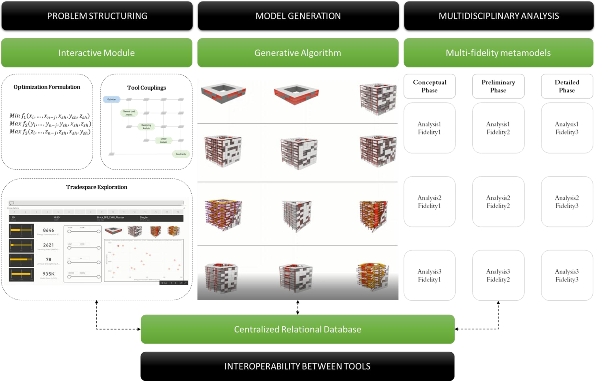
Fig. 21. Developed MDO framework with an interactive module for problem structuring, generative algorithm for model generation, multi-fidelity analysis tools to be used across multiple phases, and a centralized relational database for enhanced interoperability.
A standard operating procedure (SOP) for implementing the developed MDO framework is listed in Table 1 along with an illustration of the sequence of steps in Figure 22.

Fig. 22. Standard operating procedure (SOP) for implementing the developed MDO framework.
Table 1. Standard operating procedure for implementation of developed multi-phase concurrent coupled MDO framework to a design problem

It should be noted that Steps 3, 4, 5, 6, and 8 are automated and run in the background and are modified as and when there is a change made by the design team in the interactive module as the design progresses. However, if more design objectives apart from the initial setup are considered, then minor modifications, like mapping shared design variables and connections between newly added metamodels or analysis tools and the centralized database, need to be done as a one-time process. To illustrate how the design variables used by the metamodels of various fidelities change across multiple design phases, the general form for mathematically formulating (variables, objectives, and constraints) a sample problem with three subsystems (and three objective functions) is shown below.

Furthermore, a conceptual diagram of the SOP across the three design phases (conceptual, preliminary, and detailed) for the sample problem is shown in Figure 23. These diagrams show how the number of variables considered by the metamodels of varying fidelities vary from phase to phase. Note that the SOPs for the three design phases in Figure 23 might look similar (in print media), but the variables used in the objective functions and the metamodels are different for each design phase. For example, higher fidelity analysis tool (Fidelity 3) used during the detailed phase of design require n input variables, whereas the simpler metamodels of lower fidelity (Fidelity 1 and 2) used during the conceptual and preliminary design phases just require (n − j) and (n − k) input variables, respectively.

Fig. 23. Developed framework spanning across all three design phases using metamodels of progressive fidelity as the design progresses. x n−j, x n−k indicate dimensionality reduction in variables considered by metamodels as opposed to highest fidelity model considering x n variables.
Design of an office building
Overview of the office building design problem
The developed MDO framework was implemented to assist the design of a simple multistoried office building that adheres to minimum regulations for medium/large office buildings per ASHRAE 90.1 benchmark standards. This includes aspects such as enhanced access to natural lighting, reduced energy consumption, efficient indoor air circulation, and indoor environmental quality (Reinhart, Reference Reinhart2015; ASHRAE, 2019). Each of these aspects can be measured in terms of objective metrics such as spatial daylight autonomy, annual heating and cooling load, and energy utilization index. Modern day office buildings typically have envelope assemblies such as curtain wall systems with floor-to-ceiling windows as they are a great selling or renting point (Turan et al., Reference Turan, Chegut, Fink and Reinhart2020). Though such large windows maximize the amount of daylight penetration, they might be detrimental to the overall performance of the building in other aspects such as thermal comfort inside the building.
For example, a sample two-story office building with an area of 325 m2 was selected from the ASHRAE 90.1 energy modeling benchmark database (ASHRAE, 2020). When simulated for the spatial daylight autonomy with a wall-to-window ratio (WWR) of 50% (floor-to-ceiling curtain wall), using Pittsburgh as the design location, the design had very low daylighting values below the optimal values suggested by IESNA. In particular, IESNA recommends a minimum illuminance of 300 lux for at least half the occupied hours in a year for a building interior (also called as spatial Daylight Autonomy – sDA) to be considered well lit (ASHRAE, 2019). To achieve optimal indoor lighting levels (sDA + artificial lighting), two design strategies can be applied namely, increasing the WWR to allow more daylight penetration or increase the artificial lighting to compensate for the reduced daylighting.
Ideally, increasing the WWR helps reduce the dependence on artificial lighting and thereby reducing power consumption. Subsequently, the design was modified to have an increased WWR (75%), which resulted in better daylighting penetration, but also resulted in more heat retention thereby leading to indoor thermal discomfort. Subsequently, more cooling energy was required to compensate for the increased heat retention. A comparison of the original design (1) and modified design (2) and their respective daylighting, heat retention, and cooling energy values are shown in Figure 24.

Fig. 24. Design options 1 and 2 on the left and the plots showing sDA, heat retention and cooling energy values of (1) and (2).
It was noted that though increased WWR led to greater daylighting penetration and reduced artificial power consumption, it was detrimental in terms of an increase in cooling energy needed to dissipate excess heat retained. Hence, it is evident that trying to minimize one objective (artificial lighting power) leads to the increase of another objective (cooling energy), thereby leading to a tradeoff as shown in Figure 25.

Fig. 25. Tradeoff between artificial lighting and cooling energy for three design options with different wall-to-window (WWR) ratios.
Hence in office buildings, to maintain optimal daylighting factor, as well as thermal comfort inside the building, it is necessary to concurrently optimize the building design for daylighting, thermal loads, and energy consumption values. The developed MDO framework is demonstrated by using it to design and optimize a sample multistorey office building for multiple objectives such as thermal loads, energy, and daylighting. The various steps in implementing the MDO framework per the SOP prescribed in Table 1 in the section “Multi-phase concurrent coupled MDO framework” is discussed in the following.
MDO framework implementation
Problem structuring (Step 1 of SOP)
For the sake of this technology demonstration, the design objectives and constraints were set by the author instead of design charettes with a multidisciplinary team. The data file and score card file from the ASHRAE 90.1 database for prototype office buildings (ASHRAE, 2020) was used as a reference to frame the design objectives. Furthermore, based on the building descriptions, operating schedules, and other key modeling input information available in the data file, input variables were mathematically formulated as shown in Table 2.
Table 2. High-level input variables used in the office building design

The design location was selected to be Pittsburgh and the values for outside temperature (T o), solar azimuth angle (θ), and illuminance (E) were derived from the TMY-3 weather data file and CIE sky model for the said location, respectively. Furthermore, the indoor set point temperatures were set to be 68 degrees (T i, min) and 70 degrees (T i, max). Material values such as shading coefficients (S c,i), solar heat gain coefficients (SHGC i,), visible transmittance (VT i) of windows, and R values of the wall assembly were extracted for each window and wall assembly from the various models generated by the generative algorithm. Three objectives were defined, namely, minimizing the energy utilization index, minimizing the annual cooling load of the building, and maximizing the annual spatial daylight autonomy of the building as shown in Table 3. Actually, both heating and cooling loads were calculated as part of the overall energy utilization index of the building. However, since WWR was one of the variables which was varied parametrically, cooling load was visualized as a separate function. This helped in evaluating the impact of increases glass on heat gain inside the building and subsequent increase in cooling load.
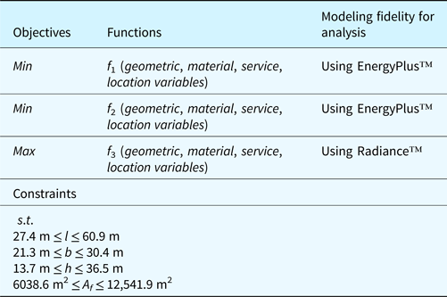
Table 3. Multidisciplinary objectives used in the office building design

As proposed in the section “Multi-fidelity metamodels for multidisciplinary analysis”, metamodels such as a modified bin method and a degree day method, and the machine learning-based daylighting estimation tool were used for facilitating faster analysis of large batches of design options for energy and daylighting during the earlier phases of design. Table 4 shows the metamodels and analysis tools of varying fidelities used for estimating the output variables across multiple design phases. The differences in variables considered by each analysis fidelity are shown in the objective functions in Tables 6, 9, and 10 representing the conceptual, preliminary, and detailed design phases, respectively.
Table 4. Multi-fidelity analysis tools and metamodels used in the office building design

Furthermore, the tool couplings between the various analysis tools were developed according to the PSM shown in Figure 26, to enable concurrent coupled MDO. Subsequently, these objectives, constraints, and the tool couplings between analysis tools of varying fidelities (metamodels) used in the different design phases were implemented computationally using the PIDO tool modeFrontier™ in the interactive module (Step 1 of SOP) (Fig. 27).

Fig. 26. PSM for concurrent coupled MDO in design of office building.

Fig. 27. Computational implementation of the PSM using PIDO tool modeFrontier™.
Model generation (Steps 2, 3, and 4 of SOP)
Once the problem was formulated mathematically, the generative algorithm (implemented using Grasshopper for Rhino™) was used to generate a catalog of design options as covered in the section “Conceptual design phase”.
Multidisciplinary analysis (Step 5 of SOP)
As mentioned in Table 4, analysis tools and metamodels of varying fidelities were used to estimate the cooling load, energy consumption, and daylighting levels (sDA) in the generated building design options. Specific to the thermal load (cooling load) and energy analysis, typically, the 3D model of the building is divided into volumetric zones based on the floor plan layout, i.e., each room into individual volumes, or a cluster of rooms with similar functions into a volume or a coarser discretization of the building into core and perimeter zone volumes. Since the generative algorithm was not programmed to generate any customized interior floor plans with interior spaces and rooms, each floor was divided into volumetric grids of 5 m × 5 m replicating thermal zones for the sake of thermal load and energy calculations. The modified bin method and the degree day method-based metamodels were used during the conceptual and preliminary design phases for thermal load analysis and energy analysis, respectively, whereas EnergyPlus™ was used for the same during the detailed phase.
Similarly, a machine learning-based daylighting prediction metamodel (Muthumanickam et al., Reference Muthumanickam, Duarte and Simpson2022a), DIVA-for-Rhino™, and Radiance™ were used as the three analysis fidelities to predict the sDA values of the design options during the conceptual, preliminary, and detailed design phases, respectively. It should be noted that the machine learning-based metamodel was developed to predict sDA values of a single floor in a building. Hence, for each design, the machine learning-based metamodel was used to predict the sDA values for each floor and an average of all floor values was calculated to arrive at the total sDA of the building.
Multidisciplinary optimization (Steps 6, 7, 8, 9, and 10 of SOP)
A conceptual representation of the overall implementation of the MDO framework for the office building design is shown in Figure 28. Furthermore, the next steps are listed in a phase-by-phase manner to explain the process flow of the framework.

Fig. 28. MDO framework implementation for the office building design.
Conceptual design phase
During the conceptual design phase, four different types of massing options, namely triangular, cubic, pentagonal, and hexagonal were modeled in Rhino™ and provided as input to the generative algorithm (implemented using Grasshopper for Rhino™). Minimum and maximum values were set for specific input sliders such as building length, width, height, the number of floors, floor-to-ceiling height, column spacing, envelope assembly wall type, WWR, and the number of glazing panes, as shown in Table 5. Apart from the individual side wall lengths of the triangular, cubic, pentagonal, and hexagonal massing, the overall length and width of the geometry were calculated as the maximum length along the longest and shortest axis passing through the centroid of the geometry. In this example, standard square grids of 6 m × 6 m, 3 m × 3 m, and 1.5 m × 1.5 m were used for columns, room, and artificial lighting layouts, respectively. The interior room walls were generated to reflect the floor slab divided into standard sized room grids with a door opening into every grid cell. Column and beam dimensions and floor slab thickness were kept at constant values in this example. Using a randomizer node in the generative algorithm to parametrically vary the values of these sliders, a sizeable catalog of 1512 building design options were generated.
Table 5. Conceptual design phase – variables

Figure 29 shows a sample subset of the design options generated using the generative algorithm. Each of these 1512 design options included LOD 350 architectural components (floor slabs, exterior walls, windows), LOD 200 structural components (columns and beams) and LOD 200 MEP components (ceiling plenum, suspended ceiling, ducts, air handling units, and lighting trays) as shown in Figure 30. Inclusion of such MEP system components during the early stages of design facilitated relatively enhanced thermal load and energy analysis during the conceptual phase, which was not possible earlier without such details. The design objectives, constraints, and the analysis tools used to estimate these output variables were defined in the PIDO tool as shown in Table 6.
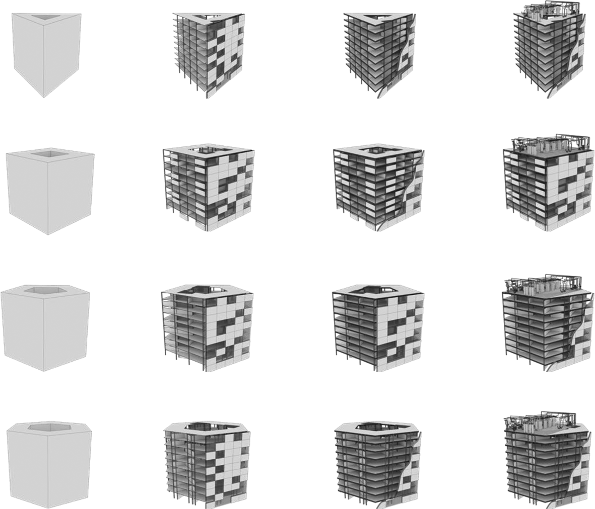
Fig. 29. 3D geometry of the building massing provided (left) and a variety of design options generated (right).

Fig. 30. Integrated building model with various systems generated when a basic massing is input into the generative design algorithm.
Table 6. Conceptual design phase – problem formulation

These tools were connected with the centralized relational database using the respective software application programming interfaces. The tool couplings between the various models, analysis tools, optimizer, tradespace exploration module, and the centralized relational database were setup using the PIDO tool modeFrontier™, as shown in Figure 31. Hence, the analysis results of all the generated design options were stored in the appropriate fields in the relational database (the master table).

Fig. 31. Tool coupling implementation between modified bin for energy and ML-based metamodels for daylighting estimation using the PIDO tool.
Upon running multidisciplinary analysis of all the generated design options using the modified bin method (for cooling load and energy estimation) and the machine learning-based metamodel (for daylighting – sDA) in this phase, the optimizer (Non-Dominated Sorting Genetic Algorithm-II or NSGA-II algorithm) converged at 296 designs that were identified as feasible options (satisfying all objectives and constraints). Furthermore, six out of the 296 design options were identified as Pareto optimal by the optimizer as shown in Table 7.
Table 7. Summary of MDO results from the conceptual design phase.

The input (Table 8) and output variables (Fig. 32) of the six Pareto optimal design options were plotted to study the tradeoffs between these designs.

Fig. 32. EUI, cooling load (CL) (left), and sDA (right) of the Pareto optimal options from the conceptual design phase.
Table 8. Summary of Pareto optimal design options from the conceptual design phase

From the above figures, it should be noted that all the Pareto optimal options have a 45-degree orientation (in reference to the True North), meaning for the given location, this orientation results in maximum daylighting while having minimal energy consumption. It should also be noted that options with more than eight floors (IDs 346, 482, 724, 972) get relatively higher amount of daylight than their counter parts (IDs 446 and 460). A plausible reason behind this might be that there is increased penetration of light to the interior of the building from lower azimuth sun angles through windows on top floors. In terms of the energy utilization index, at a first glance, it seems like there is an increase in energy consumption as the area increases. However, by comparing options 446 and 972, it was noted that both options had almost equivalent energy consumption values despite the former having a lower floor area than the latter. To further study the tradeoffs and in turn aid the MDO of the building design options, the Pareto optimal options were considered for further detailing and optimization in the preliminary design phase.
Preliminary design phase
In the preliminary design phase, the identified Pareto optimal design options from the conceptual design phase were optimized for the same three objectives but considering an increased number of variables using analysis tools relatively with sophisticated fidelities, as shown in Table 9. Specifically, the degree day method and DIVA-for-Rhino™ were used for thermal/energy analysis and daylighting analysis, respectively. As seen in Table 9, the objective functions here calculate energy consumption, cooling load, and daylighting as a function of the material and service system-oriented variables in addition to the geometric and location details. These include shading coefficient S c (0.38), HVAC schedule H s (8 hours run time), and solar heat gain coefficient SHGC (0.34).
Table 9. Preliminary design phase – problem formulation

Additionally, the bounds on the breadth and the height constraints of the building were increased as a measure for the optimizer to find options with maximal floor area. Specifically, increasing the lower bound on the height constraint led to focusing on design options with more than seven floors in the tradespace, which predominantly had an increased overall indoor daylighting level (sDA), as observed in the tradespace plots during the previous phase. Such changes to the variables, considered in estimating the output variables and the geometrical constraints, somewhat mimicked a shift in preferences as would happen in real-life design charette sessions.
The interactive problem structuring module included in the developed MDO framework helped implement such changes seamlessly across the different design phases. The PIDO component within the interactive problem structuring module also helped in interactively changing the couplings between the newly added analysis tools and connecting them with the centralized relational database (Fig. 33).
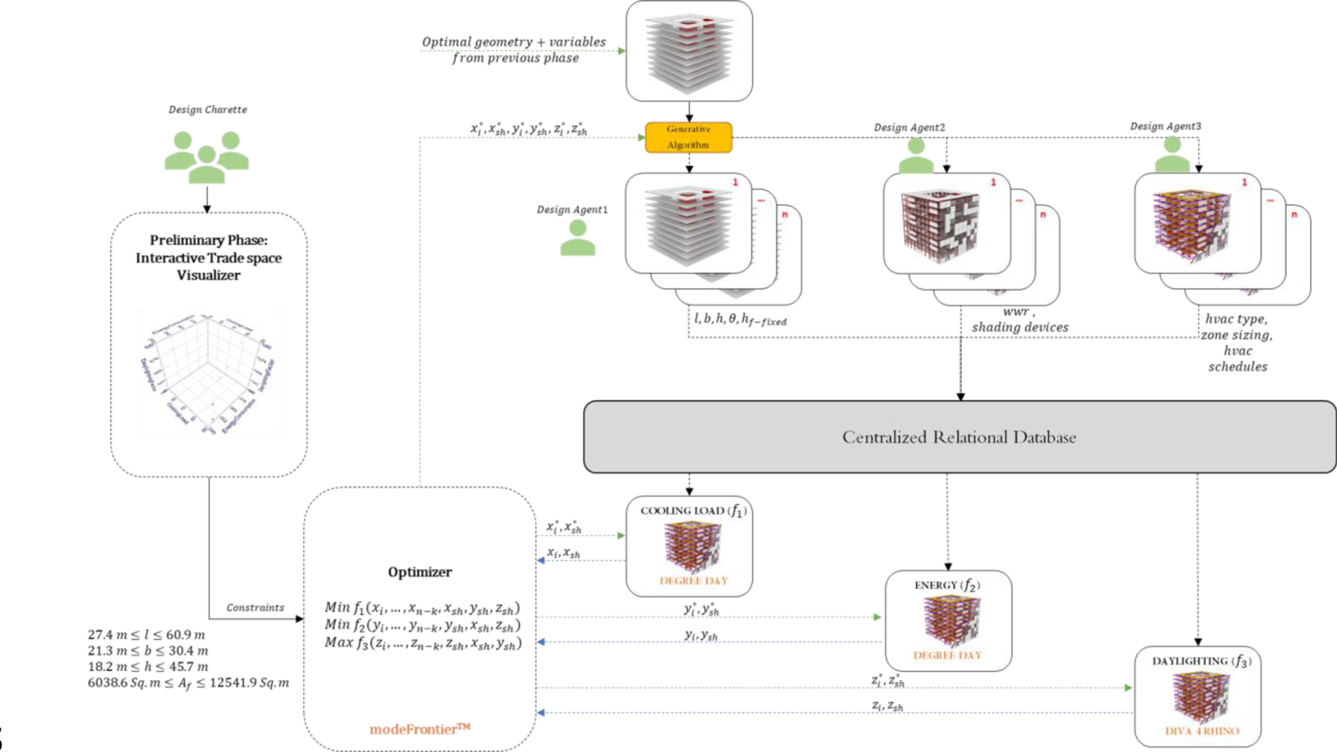
Fig. 33. Tool coupling implementation between degree day metamodel and Diva-for-Rhino™ for energy and daylighting estimation using the PIDO tool.
The optimizer (NSGA-II algorithm) identified two options as feasible (satisfying all constraints and objectives), as well as Pareto optimal.

A comparison of the thermal load, energy consumption, and sDA values of these two options estimated by the analysis tools used in the previous phase (modified bin method for thermal/energy and machine learning-based daylighting prediction tool for sDA) and those used in the current phase (degree day method for thermal/energy and DIVA-for-Rhino™ for sDA) is shown in Figure 34. It should be noted that the daylighting analysis tool in this phase used a lighting coefficient factor accounting for artificial lighting in each floor. The lighting coefficient factor was set to 50% for the sake of calculation. Hence, the sDA calculated in this phase are a summation of both natural as well as artificial lighting. Despite the change in the consideration of variables, it could be observed that the output variables estimated by both the Degree Day metamodel for energy and the DIVA-for-Rhino™ for daylighting analysis fall within a reasonable range from that predicted by the metamodels used during the previous phase. The two design options (IDs 446 and 460) were six floor and seven floor versions, respectively, with a 45-degree orientation from the True North.

Fig. 34. EUI, cooling load (CL) (left), and sDA (right) of the Pareto optimal options from the preliminary design phase.
Detailed design phase
The two Pareto optimal options (IDs 446 and 460) were further considered for more detailed evaluation using more sophisticated thermal/energy analysis and daylighting simulation tools such as EnergyPlus™ and Radiance™, respectively, as shown in Table 10.
Table 10. Detailed design phase – problem formulation
Specifically, these tools use higher-order physics equations that involve an increased number of variables, finer discretization of geometry, and robust timeseries analysis algorithms, thereby yielding more accurate results. Furthermore, the design options were detailed to have a false ceiling below the plenum with integrated lighting panels distributed at a specified distance from each other as shown in Figure 35. The optimizer was used to determine the appropriate spacing between the lighting panels (d l) which yielded an optimal distribution of indoor lighting levels. The optimizer was programmed to try out multiple variations by controlling the spacing parametrically using the generative algorithm. Unlike in the previous phase, where a generic lighting coefficient was used to account for artificial lighting, actual 3D models of lighting fixtures in the model were used in this phase. Lighting simulations in Radiance™ utilize the position and intensity of illuminance of the light fixtures, while estimating the sDA of the floor using advanced ray tracing algorithms. Since the rendering of false color maps in Radiance™ takes extensive computational time, the values of illuminance at each grid point were stored in a .csv file and a custom script in Grasshopper for Rhino™ was used to render the false color maps using these values (Fig. 35). This saved significant time in terms of simulating daylighting values for multiple options. Lighting schedule (L s) was set to 8 h and a visible transmittance (VT) value of 0.45 was used for the glazing panes. The artificial lighting consumption-related variables were also used in the heat retention/thermal load and energy consumption calculations by EnergyPlus™.

Fig. 35. Sample 3D model showing the lighting trays integrated into the false ceiling component (left); false color rendering of lighting levels generated by illuminance values from Radiance™ simulations.
Subsequently, the tool couplings between the various modeling and analysis tools, optimizer, and the interactive tradespace module were computationally implemented using the PIDO tool modeFrontier™ to automate the optimization as shown in Figure 36.

Fig. 36. Detailed design phase – framework using fidelity 3 analysis tools (EnergyPlus™ and Radiance™).
After an exhaustive variation of the input variables such as the spacing between the lighting trays and their positions, the optimizer (NSGA-II algorithm) converged on two values – 3.04 and 3.81 m spacing between the lighting trays for the two design options, respectively. Upon plotting the cooling load, energy consumption, and daylighting values estimated by EnergyPlus™ and Radiance™, against those estimated by the tools/metamodels used in the previous phases (conceptual and preliminary) for the same design options, it was observed that the values were within an acceptable range of delta, as shown in Figure 37, without any drastic differences. This further helps assert the usage of the proposed metamodels to preserve the globally optimum design options with a significant level of confidence in a multi-phase building design process.

Fig. 37. EUI, cooling load (CL) (left), and sDA (right) of the Pareto optimal options from the detailed design phase.
Detailed-extended phase
To further optimize the six and seven floor options identified as Pareto optimal options from the previous phase, the two options were mutated (modified) by parametrically controlling other variables such as wall type, glazing panels, HVAC, and lighting schedules, as shown in Table 11. This expanded the tradespace to contain 32 design options with basically the first 16 mutations evolving from design ID 446 (six floor options) and the subsequent 16 mutations evolving from design ID 460 (seven floor options). The 16 options evolving from design ID 446 are assigned new IDs as A1–A16, whereas those evolving from design ID 460 are assigned new IDs as B17–B32.
Table 11. Detailed design-extended phase – additional variables introduced

Basically, through the process of mutation, the feasible region identified in the previous phase (detailed design phase) was populated with a greater number of design options. This ensured that the objectives (energy utilization index, annual cooling load, and spatial daylight autonomy) did not exceed the previously obtained results. The output variables were estimated using the same analysis tools used during the detailed design phase (Table 12).
Table 12. Detailed design-extended phase – problem formulation

The optimizer (NSGA-II algorithm) converged on 13 design options that were identified as Pareto optimal design options. Among these 13 Pareto optimal options from the detailed-extended phase, it can be noted that majority of them are six floor options (Table 13), which are basically evolutions of design ID 446 from the detailed design phase. Only three Pareto optimal options are 7-floor options (evolutions of design ID 460).
Table 13. Comparison of 13 Pareto optimal options from the detailed-extended design phase

The energy consumption, cooling load, and daylighting levels (sDA) of the 13 Pareto optimal options are shown in Figure 38. In the previous phase (detailed design), the spatial daylight autonomy values of option 446 and 460 from the detailed design phase were 68% and 59.5%, respectively. An interesting observation in this phase was that, despite changes like the number of glazing panes and lighting schedules in this phase, almost all the Pareto optimal options yield a spatial daylight autonomy value averaging between 55% and 70% (Fig. 38). This shows that the optimizer ensures that global optimality in terms of daylighting and energy is preserved by parametrically finding the correct balance between the number of glazing panes, lighting schedules, and wall type, among other input variables.

Fig. 38. EUI, cooling load (CL) (left), and sDA (right) of the Pareto optimal options from the detailed design-extended phase.
Validation of MDO results
The results obtained by implementing the developed MDO framework to the office building design were validated by comparing them with documented benchmark standards, and the optimal options with those obtained from sequential design optimization frameworks.
Comparing with benchmark standards
The EUI and sDA of the 13 Pareto optimal solutions from the detailed design-extended phase (Table 13) were compared with baseline benchmark values prescribed by ASHRAE 90.1 (ASHRAE, 2019, 2020) and LEED v4 BD + C (Council, 2014), respectively (Fig. 39).

Fig. 39. Comparison of EUI and sDA values of 13 Pareto optimal options with ASHRAE 90.1 benchmark (left) and LEED v4 BD + C baseline (right).
In particular per ASHRAE 90.1 benchmark standards for prototype office buildings, the energy utilization values for medium and large-scale office buildings averages between 200 and 250 kWh/m2/year. Additionally, the LEED v4 standards for new building and construction (BD + C), prescribes 55% of the interior layout to have an sDA above 300 lux to be considered nominally lit and 75% as the preferred optimum. From Figure 39, it can be observed that the EUI of the Pareto optimal options does not exceed the upper bound of the benchmark EUI (250 kWh/m2/year), i.e., the options have minimal energy consumption. Similarly, it can be observed that almost all the Pareto optimal options fall within the range of 55%–75% sDA, meeting the values prescribed by the LEED v4 standard. This demonstrates that the results obtained using the developed MDO framework are well within the nominal benchmarks estimated for medium-scale office buildings and hence can be generalizable to similar design conditions.
Preservation of globally optimal solutions
Subsequently, to check if globally optimal design options were preserved across multiple phases by the developed MDO framework, the following step-by-step strategy was used:
1. The initially generated 1512 design options were sequentially optimized for cooling load, EUI, and daylighting, one after another, by using high-fidelity analysis tools (EnergyPlus™ and Radiance™) as the respective analysis tools and a set of Pareto optimal options were identified (Set A).
2. The same 1512 design options were concurrently optimized for cooling load, EUI, and daylighting by using high-fidelity analysis tools (EnergyPlus™ and Radiance™) as the respective analysis tools and a set of Pareto optimal options were identified (Set B).
3. The two Pareto optimal options (Design IDs 446 and 460) obtained from the detailed design phase by using the developed MDO framework using metamodels of varying fidelities were considered as Set C.
Then, these three sets could be compared to check if the Pareto options identified by the developed MDO framework (Set C) belonged to Set A and/or Set B. Note that Set C consisted of Pareto optimal options from the detailed design phase (Design IDs 446 and 460), instead of from the detailed-extended phase because the 13 Pareto optimal options from the detailed-extended phase were mutations of design IDs 446 and 460 created by introducing new variables. Hence, these options could not be in Set A or B.
Additionally, it should be noted with caution that though Set A consists of Pareto optimal options identified by using the highest fidelity analysis tools, there is a high probability of missing out on globally optimal design options due to the sequential optimization. Hence, it is not essential that Set C is always a subset of Set A. However, Set C should always be a subset of Set B, since Set B is the result of concurrently optimizing for all three aspects using the highest fidelity analysis tools.
After setting up the optimization formulations and computational batch analysis of the designs using the highest fidelity, the sequential and concurrent MDO identified the Pareto optimal options constituting Set A (6 designs) and Set B (5 designs), respectively, as shown in Table 14.
Table 14. Design IDs of Pareto optimal options identified by sequential MDO (Set A), concurrent MDO using high fidelity (Set B), and developed MDO framework (Set C)

It can be observed that both options 446 and 460 from Set C were part of Set B, whereas only of those (Option 460) was found in Set A. It is also interesting to note that Pareto optimal solutions (as identified in Set A) are drastically different from Sets B and C. This can be attributed to the fact that the sequential MDO while trying to achieve each objective sequentially eliminates potentially optimal candidates that might be Pareto optimal when optimized concurrently for all aspects. It should also be highlighted that Set C despite being a subset of Set B, still misses more than half of the options in Set B. Upon closer examination, it was found out that the metamodels used in the conceptual phase preserve the options in Set B as Pareto optimal, whereas the metamodels used in the preliminary design phase discard options 157, 482, and 972 as dominated solutions. Hence, it is fair to assume that the metamodels used in the preliminary phase of the proposed MDO framework have limitations in terms of preserving global optimality. However, the most interesting aspect of the developed MDO framework is its ability to identify the Pareto optimal options at a significantly lower computational time than its counterparts, as shown in Figure 40.

Fig. 40. Comparison of computational time of SDO, concurrent MDO using high-fidelity analysis, and concurrent MDO using the developed MDO framework (using multi-fidelity analysis).
It can be seen from Figure 40, that the developed MDO framework takes a cumulative computational time of 20 h and 33 min, whereas the other two methods take almost 10 days (approx.) and 27 days (approx.), respectively. Also, it should be noted that the cumulative computational time for the developed MDO framework also includes that of the detailed-extended phase, where new design mutations were developed by introducing new variables. The same initial problem formulation used for the developed MDO was used for these optimizations as well, and the optimizations were run using a high-performance computer with multiple-core, multi-thread processor (Intel® Core™ i9-10900 K 3.5 GHz) and a graphic processing unit (NVIDIA® Quadro™ RTX 5000). The energy analysis and daylighting simulations using the highest fidelity tools took several days to weeks to complete and hence were run in batches at intermittent time intervals adhering to schedule and computational resource availability constraints. The cumulative computational time of the concurrent MDO with multi-fidelity models does not include the research and development time of energy metamodels and the training (~45 h and 23 min) and validation time (~9 h and 37 min) of the ML-based daylighting metamodel. Even if these values are added, the cumulative computational time of the proposed MDO framework will still be drastically lower than its counterparts. More details about the average computational time recorded for analyzing the design options using the various metamodels are provided in Muthumanickam (Reference Muthumanickam2021).
Summary of MDO implementation to the office design problem
In summary, the developed MDO framework was implemented to aid the design process of a sample office building spanning across multiple design phases, namely, conceptual, preliminary, detailed, and detailed-extended [Fig. 28 in Section “Multidisciplinary optimization (Steps 6, 7 ,8, 9, and 10 of SOP)”]. The benefits offered by the various components of the MDO framework are listed below.
-
Generative algorithm – The generative design algorithm outlined in the section “Generative algorithm for design catalog generation” was significantly helpful in generating a large set of integrated (detailed) design options as outlined in the section “Model generation (Steps 2, 3, and 4 of SOP)”, offering parametric capabilities to the designer to control the various input variables.
-
Machine learning-based metamodel for daylighting estimation – The usage of the machine learning-based metamodel for predicting daylighting (as developed in Muthumanickam et al., Reference Muthumanickam, Duarte and Simpson2022a) enabled rapid analysis of large sets of building design options as opposed to the computational graphics intensive ray tracing-based simulations.
-
Multi-fidelity modeling approach – Subsequently, it is clear from Figure 40 that by organizing energy and daylighting analysis of varying fidelity, which also includes the developed machine learning-based metamodel for predicting daylighting, it is possible to identify Pareto optimal building design options with multidisciplinary optimality at staggeringly lower computational time.
-
Interactive problem formulation – Using the interactive features in the PIDO tool modeFrontier™ as outlined in the section “Interactive module for problem formulation, process integration, and tradespace visualization”, it was possible to change the problem formulation at ease during each phase as shown in Tables 6, 9, 10, and 12, respectively. Specifically, the change of metamodels/analysis tools at each phase required changes to the tool couplings and mapping of the variables between the modeling, analysis, and optimization tools with the centralized relational database. The interactive features and application programming interfaces of the PIDO tool helped to implement these changes using a drag-and-drop interface to define the process map [Fig. 27 in Section “Problem structuring (Step 1 of SOP)”]. Specifically, it facilitated designer intervention to enable design mutations during the detailed-extended phase. In the absence of such interactive problem structuring modules, such mutations of Pareto optimal solutions are only possible by setting up an entirely new optimization problem with revised variables and constraints specific to the detailed design phase, which requires extensive setup time (the reason why Fig. 40 does not have detailed-extended phase for frameworks other than the proposed MDO). Comparison of such setup time might have been valuable to demonstrate the benefits of the interactive problem structuring module objectively, but was not included in the original scope of this paper and hence is suggested as a potential avenue for future research.
-
Interactive tradespace exploration – The interactive tradespace exploration module of the developed MDO framework enabled interactive visualization of the tradeoffs between the various input and output variables using a variety of plots such as scatter plots and parallel coordinates plots, as shown in Figures 41 and 42. Such interactive exploration of the tradespace helped get a visual glimpse of how the tradespace progressively converged toward the Pareto optimal solutions through various phases. The web-based dashboard environment was not used much in this technology demonstration since the problem formulation and design development was a single person activity involving just the author, as opposed to a multidisciplinary environment in real-life project settings.
-
Centralized relational database – Setting up a centralized cloud-based OORDBMS database that stores data from multiple modeling tools (retrieved as IFC and translated to SQL to be stored in the OORDBMS), metamodels and tradespace analysis tools that works in tandem with the PIDO tools was helpful to automate the data exchange between multiple tools. However, relying on the promising potential of such state-of-the-art data exchange infrastructures indicated in various literature and benchmark testing (Nour, Reference Nour2009; Lee et al., Reference Lee, Jeong, Won, Cho, You, Ham and Kang2014; Li et al., Reference Li, Liu, Liu and Wang2016; Solihin et al., Reference Solihin, Eastman, Lee and Yang2017; Cho et al., Reference Cho, Won and Ham2018; Bock, Reference Bock2019; Wyszomirski and Gotlib, Reference Wyszomirski and Gotlib2020), the scope of the paper was limited to just demonstrate the setup and use of such infrastructure as one of the components within the overall MDO framework proposed and not on the rigorous and objective evaluation of the infrastructure.

Fig. 41. Parallel coordinates plot showing convergence of the tradespace toward the optimal options as the design phase progresses from conceptual to detailed-extended design.

Fig. 42. Tradespace exploration of the office building design through multiple design phases.
Conclusion, limitations, and recommendations
What is the novelty of the proposed MDO framework?
Researchers in the AEC field have contributed immensely to the research and development of topic areas such as algorithms for generating large sets of design options, metamodels for faster analysis of large sets of design options, optimization algorithms for sorting through large design spaces, and tools for visualizing tradeoffs. However, despite such developments, industry adoption of optimization frameworks by the larger AEC community is still in its infancy. For increased adoption by practitioners, it is necessary to address all the above topics collectively than a piecemeal approach of implementing these strategies as standalone methods, or tools. For example, for effective implementation of an optimization framework, it is necessary to generate many design options, to analyze them faster, to visualize the tradeoffs effectively, and to modify the optimization framework seamlessly to reflect the requirements across design phases. This shall enable visualizing more “what-if” scenarios, which in turn shall be beneficial for AEC researchers and practitioners to take informed design decisions. Hence, building on top of the valuable knowledge base established by the AEC research community on these topic areas, this paper has developed a novel MDO framework that leverages the collective benefits of generative algorithm, metamodels, database management systems, and tradespace visualization tools (see Section “Summary of MDO implementation to the office design problem”) that can be plausibly implemented across multiple design phases. This has been demonstrated using an office building example spanning across multiple phases.
What are the limitations of the proposed MDO framework and future research avenues?
Despite such potential, it is also important to acknowledge the limitations of the proposed MDO framework in its current state of implementation. Firstly, there is a probability of the global optima not being in the parametrically generated design space by the generative algorithm. Solutions for this limitation can be manifold – increase the design space to include more design options or strategically iterating feasible building design solutions to increase the chance of finding the global optima or an exhaustive enumeration of all possible building design options. However, these alternatives have deficiencies as well. For example, there is still a chance for the global optima to not be present in the design space despite an increased number of options. Convergence to a global optimum cannot be guaranteed by an iterative search either and sometimes do not even guarantee convergence at all if started in a bad location in the search space. And an exhaustive enumeration of building design options (including 3D components of multiple systems as done in this paper) is practically impossible in multi-phase design processes for two reasons, namely: (a) there is virtually no end to the number of building design options that can be generated since the design brief and boundary conditions are prone to undergo many modifications as different stakeholders enter and exit the building design process, and (b) need for exponentially high computational resource and time for generating large sets of highly detailed 3D models of buildings with multiple integrated systems. Given that this is a limitation in any optimization method (increasing the size of the design space, iterative search, and an exhaustive enumeration of design options), future research upon comparison of various search methods applied to multi-phased building design problem is recommended to gain more insights into optimization algorithm efficiency. Despite such deficiencies, trying to increase the size of the design space might always lead to a slight increase in the probability of consisting of the global optima. Hence, research pertaining to computationally inexpensive methods to generate large design spaces of highly detailed building models is a fertile ground for future research.
Secondly, the benefits of the proposed MDO framework in terms of its speed in identifying Pareto optimal solutions, comes at a cost of missing out on few Pareto optimal solutions when a higher fidelity model is used. However, this limitation is specifically associated with just the metamodels used in the preliminary design phase as discussed in Section “Preservation of globally optimal solutions”. Future research on how to improve these metamodels to better preserve global optima while not compromising on the speed benefit is required. Also, it should be noted that using the proposed metamodels as opposed to the high-fidelity models used in the sequential and concurrent MDO frameworks, as shown in Figure 40, can help understand the metamodels performance in varying MDO approaches. Moreover, since the proposed framework utilizes multiple metamodels (for energy and daylighting) at each phase, there can be multiple versions of sequential and concurrent MDO done using various combinations of these metamodels and in different orders of arrangement. This can help identify how the ordering and orchestration of the various combinations of metamodels impact the optimization results.
Thirdly, the implementation of the developed MDO framework across multiple design phases in a project requires stringent project management controls where a designated personnel or team needs to orchestrate the standard operating procedure. Additionally, the IFC to SQL translation used in this paper showcases promising potential in a well-defined problem. However, the efficiency of such a conversion in real-life projects dealing with multiple stakeholders dealing with unstructured data and formats is subject to further study. Given such requirements, it might be tedious to setup the MDO framework and a project manager responsible for orchestrating the MDO might conclude that, for a small-scale residential project with very basic technical requirements, the cost of the setup outweighs the benefits of implementation, as opposed to large-scale commercial projects. Moreover, the MDO framework might need upgrades in several aspects to perform efficiently in real-life commercial scale projects. Firstly, expanding the capability of the generative algorithm to support organic and customized shapes and interior floor layouts is needed. Secondly, better version control and tracking mechanisms are needed especially when dealing with projects involving large teams collaborating from a variety of design and engineering firms. Software platforms such as Autodesk® BIM 360™ offer insights into how changes to a single BIM model can be tracked. However, in the case of MDO, such tracking needs to be done on a large set of design options in various modeling and analysis tools, which is too complex. This requires more nuanced database management techniques and hence is a fertile area for future research. Finally, application of the developed framework to design different typologies of buildings, under varied climatic conditions, with increased objectives and constraints is needed to validate the accuracy of the optimization results across a range of project types. Rigorous analysis of how sensitive the optimization results are to change in specific building design variables might help gain more insights about the effectiveness of the optimization framework to meet performance objectives. Additionally, testing the developed MDO framework in real-life projects involving large design teams that contractually follow design and construction phases as prescribed by the AIA or RIBA Plan of Work might be beneficial for assessing the ease of use and barriers to adoption. Also, real-life projects involve incorporation of many subjective preferences in addition to the objective performance goals. Research about modes and methods to incorporate designer preferences into the MDO framework is also a very important area for future research. Overall, the components of the proposed MDO framework showcase promising potential to implement MDO to multi-phase design problems, with more room for improvements on several aspects, as mentioned above.
Data availability
More details about computational codes used for the data translation from IFC to SQL, SQL database setup, hierarchy of tables in the SQL database, and the mapping of data fields between IFC schema and the SQL database are provided in Muthumanickam (Reference Muthumanickam2021). Access to the repositories containing the code for generative algorithm, code for the development of .3js based dashboard for interactive problem structuring and SQL-based database management can be requested from the author at https://github.com/vrmnk.
Financial support
This research was supported by NSF grant CMMI-1455424 and CMMI-1455444, RSB/Collaborative Research: A Sequential Decision Framework to Support Tradespace Exploration of Multi-Hazard Resilient and Sustainable Building Designs; the National Aeronautics and Space Administration (NASA); and the Stuckeman Center for Design Computing (SCDC), Pennsylvania State University. Any opinions, findings, and conclusions or recommendations expressed in this material are those of the author(s) and do not necessarily reflect the views of the National Science Foundation.
Conflict of interest
The author(s) declare none.
Naveen Kumar Muthumanickam is a research engineer at the National Renewable Energy Laboratory (NREL), specializing in developing software and hardware technologies to enable industrialized and robotic construction of energy efficient buildings. He received his doctoral degree from Penn State, where he specialized in developing a machine learning based building design optimization framework. He was also part of the Penn State team at the finals of the NASA 3D Printed Mars habitat centennial challenge and worked on the building information modeling (BIM) based optimization and digital twin simulation for robotic concrete 3D printing. He is originally from Chennai, India with a bachelor's degree in architecture and holds an MS in architectural science and building technology from the University of Michigan, Ann Arbor. Dr. Naveen has also worked with construction technology firms such as Autodesk®, and Higharc Inc.® in the past.
Jose Pinto Duarte holds a professional degree in Architecture from TU Lisbon, and Master's and PhD degrees in Design and Computation from MIT. Currently, Dr. Duarte is the Stuckeman Chair in Design Innovation and director of the Stuckeman Center for Design Computing at Penn State, where he is Professor of Architecture and Landscape Architecture, and Affiliate Professor of Architectural Engineering and Engineering Design. Dr. Duarte was Dean of the Lisbon School of Architecture and president of eCAADe, the European association for education and research in computer-aided design. He was co-founder of Penn State's AddCon Lab and his research interests are in the use of computation to support context-sensitive design and construction. Recently, Dr. Duarte co-edited (with Branko Kolarevic) the book “Mass Customization and Design Democracy” (Routledge, NY, 2019) and his team was awarded 2nd place in the finals of the "NASA 3D Printed Mars Habitat Challenge, Phase 3.
Timothy W. Simpson is Paul Morrow Professor in Engineering Design and Manufacturing at Penn State, where he holds joints appointments with the Department of Mechanical Engineering, Department of Industrial and Manufacturing Engineering, School of Engineering Design, and Larson Transportation Institute. Dr. Simpson is also System Design Innovator at NASA Langley Research Center. His research interests are engineering design and design methodology, statistical approximations and design of experiments, and product family and product platform design. Dr. Simpson holds a BS in Mechanical Engineering from Cornell University, and an MS and PhD in Mechanical Engineering, Georgia Institute of Technology.


