


Introduction
The demand for information on ecosystem service values (ESVs), combined with a lack of time and resources required to conduct primary valuation studies, has led to common use of benefit transfer to quantify these values (Plummer Reference Plummer2009; Bateman et al. Reference Bateman, Brouwer, Ferrini, Schaafsma, Barton, Dubgaard and Hasler2011a, Reference Bateman, Mace, Fezzi, Atkinson and Turner2011b; Ferrini, Schaafsma, and Bateman Reference Ferrini, Schaafsma, Bateman, Johnston, Rolfe, Rosenberger and Brouwer2015; Johnston and Wainger Reference Johnston, Wainger, Johnston, Rolfe, Rosenberger and Brouwer2015; Richardson et al. Reference Richardson, Loomis, Kroeger and Casey2015; Johnston, Rolfe, and Zawojska Reference Johnston, Rolfe and Zawojska2018). Benefit transfer is defined as the use of research results from preexisting primary studies at one or more sites or policy contexts (called study sites) to predict welfare estimates such as willingness to pay (WTP) or related information for other, typically unstudied sites or policy contexts (called policy sites) (Johnston et al. Reference Johnston, Rolfe, Rosenberger, Brouwer, Johnston, Rolfe, Rosenberger and Brouwer2015a). Among the different approaches to benefit transfer in the literature,Footnote 1 there is emerging consensus over the advantages of methods that synthesize data from multiple sources, such as meta-analysis (e.g., Rosenberger and Phipps Reference Rosenberger, Phipps, Navrud and Ready2007; Boyle et al. Reference Boyle, Kuminoff, Parmeter and Pope2009; Johnston and Rosenberger Reference Johnston and Rosenberger2010; Kaul et al. Reference Kaul, Boyle, Kuminoff, Parmeter and Pope2013; Rolfe, Brouwer, and Johnston Reference Rolfe, Brouwer, Johnston, Johnston, Rolfe, Rosenberger and Brouwer2015; Johnston, Rolfe, and Zawojska Reference Johnston, Rolfe and Zawojska2018).
The most common applications of meta-analysis for ESV benefit transfer involve meta-regression models (MRMs). These models generate parametric functions that characterize the systematic influence of economic, ecological (or resource), beneficiary (population), and primary study attributes on comparable measures of value.Footnote 2 The resulting functions are used to predict values at policy sites where original valuation studies have not been conducted. Explanatory variables in these MRMs can link directly to biophysical models and enable adjustments in ESV estimates for the attributes of ecosystems, regions, populations, and policy contexts. There are many examples of such MRMs applied to different types of environmental and ecosystem service improvements including water quality (Johnston, Besedin, and Stapler Reference Johnston, Besedin and Stapler2017), recreational fishing (Johnston et al. Reference Johnston, Ranson, Besedin and Helm2006), forest recreation (Zandersen and Tol Reference Zandersen and Tol2009), and wetlands-provided ecosystem services (Brander et al. Reference Brander, Bräuer, Gerdes, Ghermandi, Kuik, Markandya and Navrud2012), among many others.Footnote 3
Despite this work, further advances in methods and understanding are required if meta-analyses are to be relied on for widespread ESV prediction, particularly within large-scale applications. The capacity of MRMs to support valid and reliableFootnote 4 benefit transfers depends on multiple criteria, including the use of appropriate econometrics (Nelson and Kennedy Reference Nelson and Kennedy2009; Boyle and Wooldridge Reference Boyle and Wooldridge2018) and specifications able to accommodate expected patterns such as the sensitivity of values to scope, scale, and spatial dimensions (Johnston, Besedin, and Stapler Reference Johnston, Besedin and Stapler2017; Johnston, Besedin, and Holland Reference Johnston, Besedin and Holland2018; Johnston, Rolfe, and Zawojska Reference Johnston, Rolfe and Zawojska2018; Kling and Phaneuf Reference Kling and Phaneuf2018; Newbold et al. Reference Newbold, Simpson, Massey, Heberling, Wheeler, Corona and Hewitt2018a, Reference Newbold, Walsh, Massey and Hewitt2018b; Smith Reference Smith2018).Footnote 5 ESV applications are often deficient in these areas (Bateman et al. Reference Bateman, Mace, Fezzi, Atkinson and Turner2011b; Richardson et al. Reference Richardson, Loomis, Kroeger and Casey2015; Johnston, Rolfe, and Zawojska Reference Johnston, Rolfe and Zawojska2018). Invariance of transferred welfare estimates to dimensions such as these can signal a lack of construct validity (Johnston, Besedin, and Stapler Reference Johnston, Besedin and Stapler2017).Footnote 6 The estimation of MRMs for ecosystem service valuation also requires robust primary study data for the type of values under study, with sufficient study reporting for metadata development (Loomis and Rosenberger Reference Loomis and Rosenberger2006).
In addition, multiple procedures are required to predict and aggregate values for policy sites using MRM or other transfer functions. These procedures must address challenges such as (1) linking biophysical information on the scope and scale of environmental changes to MRM functions, (2) accounting for the extent of the market and other spatial dimensions of households and environmental changes, (3) addressing practical dissimilarities or gaps between MRM variables and measurable conditions at the policy site, (4) accounting for the systematic influence of methodological factors on value estimates, and (5) ensuring that the resulting predictions have theoretical and empirical properties required to ensure validity for the intended uses.
Concerns such as these are sometimes overlooked in the ecosystem services valuation literature, leading to many MRMs that—despite having superficially acceptable statistical performance—are poorly suited to credible benefit transfer applications. As noted by Johnston, Rolfe, and Zawojska (Reference Johnston, Rolfe and Zawojska2018, p. 202), “Many applications [of meta-analysis in the ecosystem services] literature lack minimal properties necessary to promote valid and reliable [benefit transfer] estimates.” Even if the underlying MRM is suitable for this purpose, valid transfers also depend on the post-estimation procedures used to predict ESVs from the estimated benefit function. These issues are seldom discussed. The academic literature focuses primarily on estimation and interpretation of the underlying MRMs rather than the evaluation and use of these models for benefit transfer. The practical steps and challenges involved in benefit prediction and aggregation using these MRMs—or properties of the resulting value estimates—are not often considered in detail.
This article discusses prospects and challenges related to the use of MRMs for benefit transfer. We begin with a summary of key issues and challenges associated with the use of MRMs to forecast values for large-scale ESVs, including post-estimation issues given sparse attention in the literature. We illustrate these issues using a meta-analysis of WTP for water quality changes that support aquatic ecosystem services (Johnston, Besedin, and Stapler Reference Johnston, Besedin and Stapler2017) and the application of this model to estimate aggregate water quality benefits under alternative riparian buffer restoration scenarios in New Hampshire's Great Bay Watershed. The MRM is reviewed with respect to key validity criteria to highlight both advantages and limitations of the model. Benefit transfers from this MRM are compared for multiple scenarios, scopes, and scales of environmental improvement in the case study area, aggregated over different market extents.
The goal of this illustration is practical. Unlike publications that focus on MRM estimation and interpretation, here we emphasize often-unreported steps and choices associated with the use of MRM benefit functions for ESV prediction, as well as patterns in the resulting welfare forecasts. Attention is given to topics such as the consistency between variables used in published MRMs (typically reflecting data reported by primary studies in the metadata) and biophysical data of the type available to quantify ecosystem service changes. We also consider the properties and construct validity of the resulting value predictions. These illustrations highlight the advantages of MRM benefit transfers together with challenges and data needs.
Meta-Analysis Properties and Benefit Transfer Validity
The potential advantages of meta-analysis for benefit transfer are established in the literature (Rosenberger and Phipps Reference Rosenberger, Phipps, Navrud and Ready2007; Nelson and Kennedy Reference Nelson and Kennedy2009; Rosenberger and Johnston Reference Rosenberger and Johnston2009; Johnston and Rosenberger Reference Johnston and Rosenberger2010; Kaul et al. Reference Kaul, Boyle, Kuminoff, Parmeter and Pope2013; Rolfe, Brouwer, and Johnston Reference Rolfe, Brouwer, Johnston, Johnston, Rolfe, Rosenberger and Brouwer2015; Boyle and Wooldridge Reference Boyle and Wooldridge2018; Johnston, Rolfe, and Zawojska Reference Johnston, Rolfe and Zawojska2018). Meta-regression analyses synthesize the results of multiple prior studies into a single set of parametric predictors that can be used within benefit transfer, providing a means to ground transfers in a broad base of prior information.Footnote 7 The resulting function allows predicted values to be tailored to the needs of particular policy evaluations.Footnote 8
There is emerging consensus over the advantages of methods that synthesize data from the literature in this way, including potential improvements in benefit transfer reliability—or reductions in generalization error (e.g., Rosenberger and Phipps Reference Rosenberger, Phipps, Navrud and Ready2007; Boyle et al. Reference Boyle, Kuminoff, Parmeter and Pope2009; Johnston and Rosenberger Reference Johnston and Rosenberger2010; Johnston and Thomassin Reference Johnston and Thomassin2010; Kaul et al. Reference Kaul, Boyle, Kuminoff, Parmeter and Pope2013; Rolfe, Brouwer, and Johnston Reference Rolfe, Brouwer, Johnston, Johnston, Rolfe, Rosenberger and Brouwer2015; Johnston, Rolfe, and Zawojska Reference Johnston, Rolfe and Zawojska2018). The capacity of MRMs to synthesize information across studies that vary across commodity, site, policy, and population factors can obviate the need to find one study that is a close match to the policy site across all dimensions (Stapler and Johnston Reference Stapler and Johnston2009). Meta-analytic transfers can also reduce the risk of error caused by the use of a study site that differs from the policy site in influential ways or a primary study that suffers from measurement error, and can help diagnose and ameliorate the effect of selection biases in the literature (Stanley Reference Stanley2005; Hoehn Reference Hoehn2006; Rosenberger and Johnston Reference Rosenberger and Johnston2009; Boyle and Wooldridge Reference Boyle and Wooldridge2018).
Despite these advantages, the ability of an MRM to provide valid and reliable predictions depends on multiple factors, including the procedures used for data synthesis, statistical analysis, value prediction, and benefit aggregation (Smith and Pattanayak Reference Smith and Pattanayak2002; Nelson and Kennedy Reference Nelson and Kennedy2009; Boyle et al. Reference Boyle, Parmeter, Boehlert and Paterson2013; Boyle, Kaul, and Parmeter Reference Boyle, Kaul, Parmeter, Johnston, Rolfe, Rosenberger and Brouwer2015; Nelson, Reference Nelson, Johnston, Rolfe, Rosenberger and Brouwer2015; Boyle and Wooldridge, Reference Boyle and Wooldridge2018; Johnston, Rolfe, and Zawojska Reference Johnston, Rolfe and Zawojska2018). Considerations such as these are frequently overlooked in the ecosystem services literature, leading to transfers that violate conditions for construct validity in welfare estimates (Plummer Reference Plummer2009; Bateman et al. Reference Bateman, Mace, Fezzi, Atkinson and Turner2011b; Johnston and Wainger Reference Johnston, Wainger, Johnston, Rolfe, Rosenberger and Brouwer2015; Richardson et al. Reference Richardson, Loomis, Kroeger and Casey2015).
Prior reviews of MRMs in environmental economics find that many violate best practice guidelines for econometric analysis (Nelson and Kennedy Reference Nelson and Kennedy2009). Boyle and Wooldridge (Reference Boyle and Wooldridge2018) discuss additional issues related to metadata construction and MRM specification, as related to the validity and reliability of predictions. They distinguish between MRMs used to understand a body of empirical literature and those used to predict values. Among their key findings is that “no single estimated meta-equation is suitable for prediction in all benefit-transfer applications” (Boyle and Wooldridge Reference Boyle and Wooldridge2018, p. 633). Care must be taken to construct metadata and specify equations to predict values grounded in a consistent theoretical definition and commodity type. Hence, “a one-size-fits-all use of an estimated meta-equation to support benefit transfers is likely not appropriate” (Boyle and Wooldridge Reference Boyle and Wooldridge2018, p. 633). Kling and Phaneuf (Reference Kling and Phaneuf2018), Newbold et al. (Reference Newbold, Walsh, Massey and Hewitt2018b), and Moeltner (Reference Moeltner2019) consider whether and when MRM specifications should be further restricted to impose theoretical properties such as adding-up on benefit transfers, in some cases reaching contrary conclusions.Footnote 9
Among commonly acknowledged requirements for valid valuation via MRMs is at least a minimal degree of commodity and welfare consistency across metadata observations (Smith and Pattanayak Reference Smith and Pattanayak2002; Bergstrom and Taylor Reference Bergstrom and Taylor2006; Loomis and Rosenberger Reference Loomis and Rosenberger2006, Nelson and Kennedy Reference Nelson and Kennedy2009; Johnston and Rosenberger Reference Johnston and Rosenberger2010; Boyle and Wooldridge Reference Boyle and Wooldridge2018; Johnston, Rolfe, and Zawojska Reference Johnston, Rolfe and Zawojska2018). Moeltner and Rosenberger (Reference Moeltner and Rosenberger2014, p. 470) characterize commodity consistency as a situation in which “basic commodities under consideration [within the metadata] must be essentially equivalent.” Welfare consistency implies parallel consistency in the theoretical welfare constructs measured across observations. Many ESV MRMs are estimated using primary study data sets that pool value metrics that have no such relationship, such as estimates of consumer value, producer value, and measures that do not reflect welfare-theoretic values of any type. Prior MRMs have also pooled value estimates linked to dissimilar goods and services such as recreation, flood control, fisheries production, carbon sequestration, raw material provision, nutrient cycling, water supply, existence, aesthetics, and others (Johnston, Rolfe, and Zawojska Reference Johnston, Rolfe and Zawojska2018). The lack of metadata consistency within such models raises validity concerns (Bergstrom and Taylor Reference Bergstrom and Taylor2006)—neither theory nor economic intuition justifies the inclusion of such dissimilar welfare measures within the estimation of a single meta-analytic value function.Footnote 10
Any remaining differences in commodity, site, or population characteristics that might influence value must be captured using right-hand side variables in the MRM. However, even similar environmental changes may be defined in different ways across the literature, and reconciling these measurements across studies is not always straightforward (Smith and Pattanayak Reference Smith and Pattanayak2002; Johnston et al. Reference Johnston, Besedin, Iovanna, Miller, Wardwell and Ranson2005; Van Houtven, Powers, and Pattanayak Reference Van Houtven, Powers and Pattanayak2007; Rolfe, Brouwer, and Johnston Reference Rolfe, Brouwer, Johnston, Johnston, Rolfe, Rosenberger and Brouwer2015). This can lead to trade-offs between the number of studies (N) and independent variables (K) within an MRM (Moeltner, Boyle, and Paterson Reference Moeltner, Boyle and Paterson2007, p. 252)—“should the researcher discard explanatory variables that are not common to all studies (thus preserve N at the cost of K) or discard observations that do not include all key regressors (thus preserve K at the cost of N)?” Accuracy can be diminished if the resulting variables are quantified in low-resolution or categorical terms (e.g., high, medium, and low) (Johnston et al. Reference Johnston, Schultz, Segerson, Besedin and Ramachandran2012; Johnston, Besedin, and Stapler Reference Johnston, Besedin and Stapler2017). Moreover, the usefulness of any valuation exercise is reduced if variables are defined in ways that cannot be directly linked to the quantitative biophysical, health, or engineering outputs used to quantify effects for policy analysis (Loomis and Rosenberger Reference Loomis and Rosenberger2006; Johnston et al. Reference Johnston, Schultz, Segerson, Besedin and Ramachandran2012; Schultz et al. Reference Schultz, Johnston, Segerson and Besedin2012; Boyd et al. Reference Boyd, Ringold, Krupnick, Johnston, Weber and Hall2016).
The validity of MRM benefit transfers further depends on the extent to which these transfers reflect theoretical patterns expected in welfare estimates (Kling and Phaneuf Reference Kling and Phaneuf2018). For example, microeconomic theory suggests that predictions of per household WTP for most ecosystem service changes should respond to the scope and scale of the change, as well as substitutes and spatial dimensions. For nonmarginal changes, diminishing marginal values are typically expected. Hence, linear “scaling-up” of value predictions is unlikely to produce valid estimates, particularly when scaled to a large degree (Bockstael et al. Reference Bockstael, Freeman, Kopp, Portney and Smith2000; Bateman et al. Reference Bateman, Mace, Fezzi, Atkinson and Turner2011b; Brander et al. Reference Brander, Bräuer, Gerdes, Ghermandi, Kuik, Markandya and Navrud2012; Johnston and Wainger Reference Johnston, Wainger, Johnston, Rolfe, Rosenberger and Brouwer2015). Theory also suggests that most ESVs should be sensitive to household income, among other population attributes, although naïve income adjustments may not always improve transfers (Johnston and Duke Reference Johnston and Duke2010). Expectations such as these influence the type of MRM specifications required for validity.
A final set of questions and concerns—and those perhaps given least attention in the literature—relates to the post-estimation steps required to predict and aggregate values from a metafunction. These procedures can have a profound impact on benefit predictions. For example, as shown by Johnston, Besedin, and Ranson (Reference Johnston, Besedin and Ranson2006) for the treatment of primary study methodological variables when predicting benefits, the use of ad hoc procedures can cause WTP predictions to vary more than 15-fold. This sensitivity can be reduced with best practices for post-estimation value prediction (Stapler and Johnston Reference Stapler and Johnston2009; Boyle and Wooldridge Reference Boyle and Wooldridge2018).
One often overlooked post-estimation concern relates to variable measurement conventions applied in the MRM (discussed previously), including those used to quantify the biophysical scope and scale of ecosystem service changes. First, one must assess whether the ecosystem service of interest at the policy site is a good match for the service(s) covered by the MRM. Assuming a good match exists, one must then link the relevant biophysical changes predicted at a policy site to ecosystem service measures used within the existing MRM and obtain any required data or biophysical model outputs.
For example, Rolfe, Brouwer, and Johnston (Reference Rolfe, Brouwer, Johnston, Johnston, Rolfe, Rosenberger and Brouwer2015) meta-analyze per household WTP per kilometer of river in “good” health, where studies in the metadata define good health using different types of biophysical criteria. The usefulness of such results for benefit transfer requires a defensible and replicable way to predict this outcome (kilometers in good health) using biophysical information available to policy analysts. Even for a given benefit function, different analyst assumptions regarding biophysical measures or indices can lead to different benefit predictions. Walsh and Wheeler (Reference Walsh and Wheeler2013, p. 81) demonstrate that different assumptions regarding the mathematical structure of water quality indices “can have a profound effect on benefits.” In addition, MRM variables are often defined in ways that are biophysically ambiguous, potentially exacerbating the challenge of linking measured policy effects to MRM benefit estimates.
A second post-estimation concern relates to the role of spatial dimensions in benefit estimation, including the assigned extent of the market for benefit prediction and aggregation. As noted by Bateman et al. (Reference Bateman, Day, Georgiou and Lake2006, Reference Bateman, Brouwer, Ferrini, Schaafsma, Barton, Dubgaard and Hasler2011a), Schaafsma (Reference Schaafsma, Johnston, Rolfe, Rosenberger and Brouwer2015), Johnston et al. (Reference Boyle, Kotchen and Smith2017), and Johnston, Besedin, and Holland (Reference Johnston, Besedin and Holland2018), choices such as these can swamp the effects of other procedural choices in benefit transfer. A related challenge is that—depending on the MRM specification—average and aggregate benefits may vary depending on whether average benefits are predicted for one large market or multiple component submarkets. In such cases, is it sufficient to predict values assuming one constant “average” ecosystem service change and baseline over one large market area? Or, should values be predicted for smaller areas, reflecting the specific changes and baselines in those areas? If one chooses the latter approach, what is the appropriate size of the subareas to be considered? When values depend on spatial dimensions (Schaafsma Reference Schaafsma, Johnston, Rolfe, Rosenberger and Brouwer2015; Glenk et al. Reference Glenk, Johnston, Meyerhoff and Sagebiel2019), predicted aggregate values for average environmental changes everywhere will not, in general, be equal to the same values averaged over the population for spatially heterogeneous changes. Similar questions apply to other contextual considerations that vary over space such as income and substitutes.
A third consideration is whether the desired policy site ESV scenarios are suitable for valuation using the MRM in question. For example, would a particular scenario require values to be predicted outside the data range of the primary study metadata? With a few exceptions, the literature provides little guidance for these post-estimation procedures, leading to wide variation in applied practice. Compounding this challenge is a tendency of these procedures and assumptions to remain unreported, leading to lack of methodological transparency.
Illustrative Application: Predicting Water Quality Benefits from Buffer Restoration
This section illustrates the use of an applied MRM for ESV benefit transfer. Among the goals of this illustration are to (a) demonstrate the characteristics of the MRM required for valid benefit transfers, (b) clarify the post-estimation steps and choices required to generate and evaluate predictions using the model, and (c) discuss the advantages and disadvantages of the resulting benefit predictions. The intent is to clarify often-undocumented properties and practices that affect transfer value validity. The empirical case study analysis implements a benefit transfer to quantify per household and aggregate market WTP associated with water quality improvements of the type that could result from the restoration of vegetated buffers within New Hampshire's Great Bay watershed. We use an existing MRM for this purpose to enable focus on model evaluation and post-estimation benefit transfer, rather than on estimation of an original MRM.
Benefits are predicted using an application of the MRM estimated by Johnston, Besedin, and Stapler (Reference Johnston, Besedin and Stapler2017). This model was designed to support benefit transfer for water quality improvements in U.S. water bodies including rivers, lakes, and estuaries and reflects the type of MRM used by the U.S. Environmental Protection Agency (U.S. EPA) for regulatory analysis (U.S. EPA 2009a, 2010, 2012, 2015; Griffths et al. Reference Griffiths, Klemick, Massey, Moore, Newbold, Simpson, Walsh and Wheeler2012). The metadata were drawn from primary stated preference studies that estimated total (use and nonuse) per household WTP for water quality changes in water bodies that support ecosystem services including aquatic life, recreational uses (e.g., fishing, boating, and swimming), and nonuse values.Footnote 11 This MRM and metadata have been used as the basis for multiple prior validity tests and analyses (e.g., Newbold et al. Reference Newbold, Walsh, Massey and Hewitt2018b; Moeltner Reference Moeltner2019), so that the underlying properties of the meta-analysis are well known. As such, this MRM provides an established foundation from which to demonstrate an applied benefit transfer.
Grounded in this MRM, we present the process used to apply the resulting transfer function, along with assumptions and implications for valid benefit transfer. To illustrate how transferred WTP estimates vary across different types of water bodies, we predict values for improvements to the Great Bay and two of its tributaries, the Squamscott River and Exeter River. Values for improvements to each of these areas are predicted independently, holding conditions at other areas constant. We consider various scenarios of water quality change for these water bodies, based on current baseline quality. We also consider values predicted and aggregated over different market areas. The goal is to consider the responsiveness of WTP estimates to factors such as scope, scale, extent of the market, and baseline condition. We also describe the water quality index (WQI) used to quantify water quality baselines and changes within the MRM, as well as how the index is defined as a function of water quality parameters.
The Meta-Regression Model
As described by Johnston, Besedin, and Stapler (Reference Johnston, Besedin and Stapler2017), all observations in the original metadata were identified and coded following the guidelines of Stanley et al. (Reference Stanley, Doucouliagos, Giles, Heckemeyer, Johnston, Laroche and Nelson2013). To ensure welfare consistency, observations were restricted to U.S. studies that estimated total (use and nonuse) value, used established stated preference methods, reported comparable Hicksian WTP measures, and provided sufficient detail to verify that valuation methods met minimum quality standards. To ensure commodity consistency, studies were limited to those for which per household WTP estimates could be mapped to water quality changes measured on a standardized 100-point WQI that relates pollutant concentrations to water body suitability for human uses (Walsh and Wheeler Reference Walsh and Wheeler2013). The final metadata included 140 unique observations from 51 stated preference studies published between 1985 and 2013 (Table 1).
Table 1. Primary Studies in the Metadata (willingness to pay [WTP] is per household per year in 2007 USD)
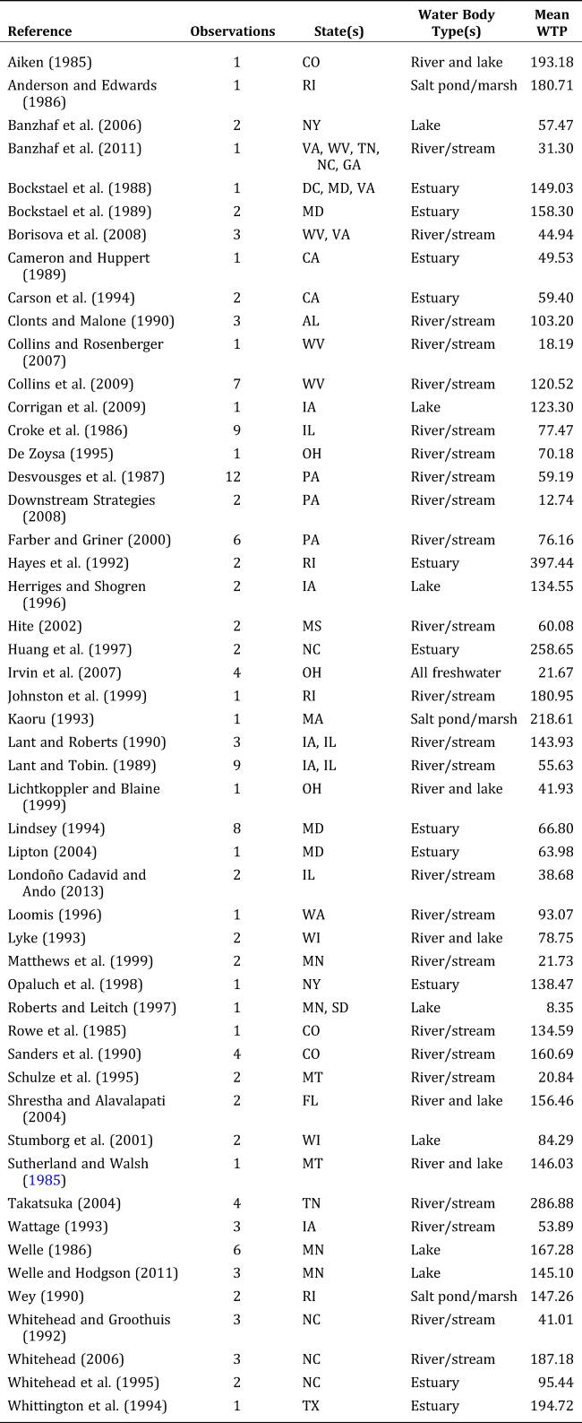
Note: Complete citations to these referenced works are provided by Johnston, Besedin, and Stapler (Reference Johnston, Besedin and Stapler2017).
The dependent variable in the MRM is the natural log of per household WTP for water quality improvements specified in each original study, with all values adjusted to 2007 USD (these values are subsequently updated to 2016 USD as discussed in Implementing the Benefit Transfer below). Independent variables expected to explain variation in this value measure (and included in the model) characterize (1) the geographic region and affected aquatic resources, (2) affected ecosystem services, (3) populations whose values were measured, (4) baseline resource condition and water quality change, (5) potential substitute resources and complementary land uses, and (6) the primary study methodology and year (Table 2). Emphasis was given to core economic and resource variables directly relevant to benefit transfer. To construct the data set, variables reported directly by primary studies were supplemented with data on study sites, beneficiary populations, and water bodies extracted from readily available national data sets.Footnote 12
Table 2. Meta-Analysis Variable Descriptions and Mean Metadata Values
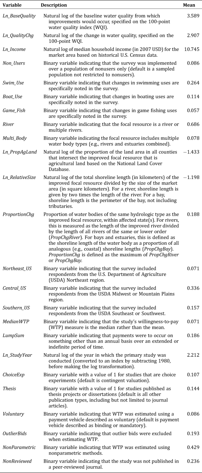
Among key variables in the MRM is that characterizing the scope (or size) of the water quality change, measured as a natural log (Ln_QualityChg). The model also includes a spatial index variable (Ln_RelativeSize) that characterizes the size of the affected water body measured using shoreline length in kilometers (geospatial scale), relative to the size of the sampled market area measured in square kilometers (market extent). This specification enables the marginal effect of water body size on WTP to decline as size of the sampled market area increases, and vice versa. The inclusion of market area in this composite index also provides a means to proxy for the effect of distance decay on value, as larger sampled market areas generally imply greater distances to affected water bodies, ceteris paribus (Johnston, Besedin, and Stapler Reference Johnston, Besedin and Stapler2017).
To characterize the scope of proportional effects on regional (potentially substitute) water bodies, the variable ProportionChg measures the proportion of water bodies (of the same hydrologic type) affected by the water quality change, within each state. Potential land use complements to water quality (specifically, the lack of complementary land uses) are characterized using Ln_PropAgLand, representing the (natural log of the) proportion the affected area with agricultural land use.Footnote 13 The model also includes variables characterizing affected uses (or ecosystem services) mentioned in each primary study such as fishing and swimming (or nonuse only), as well as indicators identifying the region of the United States where changes occurred.
The MRM is estimated using unweighted random effects ordinary least squares with robust standard errors, allowing for cross-sectional correlation among observations from the same study (Nelson and Kennedy Reference Nelson and Kennedy2009).Footnote 14 The model is specified as

where $\bar{y}_{js}$ is the welfare measure for observation s in study j (the natural log of mean or median WTP per household for the specified water quality change), and $\bar{x}_{js}$
 is the vector of independent variables. This vector includes natural logs of household income (Ln_Income), water quality change and baseline (Ln_QualityChg; Ln_BaseQuality), relative geospatial scale (Ln_RelativeSize), and agricultural land proportion (Ln_PropAgLand). Other variables enter linearly.Footnote 15 The vector β represents a conforming parameter vector. Following standard specifications, εjs = e js + u s, where u s represents a systematic, normally distributed, study-level random effect with E(u s) = 0 and Var(u s) = σu2; and e js is a standard iid (independent and identically distributed) estimation level error, distributed with a zero mean and constant variance σe2.
Results are shown in Table 3. Parameter estimates are jointly significant at p<0.01 (χ2 = 729.61, df = 24), with an R2 of 0.633. Signs of significant parameter estimates match those suggested by theory. For example, WTP is positively related to the scope of water quality change (Ln_QualityChg), household income (Ln_Income), improvements to larger water bodies and samples over smaller market extents (Ln_RelativeSize), and improvements that affect a larger proportion of surrounding waters (ProportionChg). WTP is negatively related to improvements in more agricultural areas (Ln_PropAgLand) and samples limited to nonusers (Non_Users). The functional form implies diminishing marginal utility with regard to scope and scale. Other properties of the underlying MRM are discussed by Johnston, Besedin, and Stapler (Reference Johnston, Besedin and Stapler2017).
Table 3. Meta-Regression Results—Random Effects Model (Johnston, Besedin, and Stapler et al. Reference Johnston, Besedin and Stapler2017)

Note: *** p < 0.01, ** p < 0.05, * p < 0.10.
Implementing the Benefit Transfer
Estimating the MRM is only the first step in benefit transfer. Few articles discuss the procedures required to move from the estimated MRM to benefit transfer predictions, along with the choices and challenges that are involved. The objective of this section is to make these procedures transparent and replicable. The basic steps of an ESV transfer are described by Johnston and Wainger (Reference Johnston, Wainger, Johnston, Rolfe, Rosenberger and Brouwer2015).Footnote 16 Two initial steps include establishing the need for benefit transfer and developing the conceptual foundation for the exercise. The latter involves development of an implicit or explicit “conceptual model of relationships between ecosystem processes and human benefits, including the biophysical pathways through which benefits are realized and their connections to different beneficiary groups” (Johnston and Wainger Reference Johnston, Wainger, Johnston, Rolfe, Rosenberger and Brouwer2015, p. 247). Such a model should clarify the linkages between actions, changes in ecosystem services, and the effect of these changes on utility (Bateman et al. Reference Bateman, Mace, Fezzi, Atkinson and Turner2011b; Olander et al. Reference Olander, Johnston, Tallis, Kagan, Maguire, Polasky, Urban, Boyd, Wainger and Palmer2018). This conceptual model is developed within a valuation context in which management scenarios, ecosystem services, and affected populations can be defined. ESVs at policy sites are predicted conditional on a set of biophysical changes in ecosystem services. These changes can be quantified in various ways, including biophysical models, field observations, or the use of hypothetical scenarios.
Here, we investigate three distinct water-quality change scenarios for three different water bodies within the Great Bay watershed of New Hampshire, USA (Figure 1): the Great Bay Estuary itself, not including tributaries (Figure 2), and the freshwater and tidal portions of the Exeter-Squamscott tributary (Figure 3). These define the geospatial scale of changes to be considered. Market extents must also be defined—the location of households for whom values are estimated. For the Great Bay Estuary, we evaluate WTP over three different market areas: (1) residents in NH towns immediately adjacent to the bay (Figure 2), (2) residents of NH towns within the entire Great Bay watershed (Figure 1), and (3) all residents of New Hampshire (Figure 1, inset). For the Exeter-Squamscott River, we evaluate WTP for residents in towns adjacent to the upper or lower portion of the river, respectively (Figure 3). The water quality improvements to be considered include those that could potentially arise because of intensive restoration of vegetated riparian buffers around the focal water bodies, of the general type discussed by Johnston, Holland, and Yao (Reference Johnston, Holland and Yao2016) for the nearby Wells National Estuarine Research Reserve. Restoration of this type can improve water quality through various processes, such as nutrient uptake, reduction of storm-water runoff, and shoreline stabilization by riparian buffer vegetation.

Figure 1. Great Bay Watershed in New Hampshire, USA


Figure 3. Exeter-Squamscott River Watershed, a Subwatershed in the Southern Portion of the Great Bay Watershed (Hydrologic Unit Code 0106000308)
Quantifying Water Quality Change
A core component of any ESV benefit transfer is quantification of the change in ecosystem services for which values are to be estimated, in units that are meaningful for value prediction. This requires the definition of biophysical units that link ecosystem service changes at the policy site to variables in the MRM that characterize baselines and changes (i.e., scope). Here, this is done using a standard 100-point WQI to quantify water quality changes of the type that could occur because of riparian buffer restoration (Walsh and Wheeler Reference Walsh and Wheeler2013). As described by Johnston, Besedin, and Holland (Reference Johnston, Besedin and Holland2018), WQIs combine information on physical and chemical water quality parameters into a single index linked to the ecosystem services or uses provided by a water body (Abbasi Reference Abbasi2012; Walsh and Wheeler Reference Walsh and Wheeler2013; Van Houtven et al. Reference Van Houtven, Mansfield, Phaneuf, von Haefen, Milstead, Kenney and Reckhow2014). They are among the most common means to measure water quality for valuation and benefit transfer (Griffiths et al. Reference Griffiths, Klemick, Massey, Moore, Newbold, Simpson, Walsh and Wheeler2012; Walsh and Wheeler Reference Walsh and Wheeler2013). Here we apply the WQI methodology and classification of U.S. EPA (2009b), adapted from Cude's (Reference Cude2001) Oregon Water Quality Index.
Implementing the WQI to quantify baselines and changes entails three steps: (1) obtaining pollutant data and projections for the water body, (2) transforming these data into subindex values, and (3) combining the subindex values into an aggregate WQI score. The pollutants used by the WQI, along with their required units of measure and associated WQI subindex weights, are shown in Table 4. To establish baselines, pollutant data were obtained from the New Hampshire Department of Environmental Services (NHDES). These data were averaged across all sampling periods and monitoring stations for several NHDES Water Quality Assessment Units in each of our three focal water bodies to produce WQI pollutant parameter values for each pollutant subindex.Footnote 17 These pollutant parameter values were transformed into corresponding subindex values using functions and thresholds in Table 5.Footnote 18
Table 4. Water Quality Index (WQI) Pollutants, Concentration Units, and Index Weights

Table 5. Water Quality Index Parameter-Subindex Equations

Note: See Table 4 for definition of abbreviations.
Finally, the subindex values weights were used to calculate the WQI for each major water body using the weighted geometric mean, as described by Walsh and Wheeler (Reference Walsh and Wheeler2013),

where Q i is the calculated water quality subindex for parameter i and W i is the weight of the ith parameter from Table 4. The resulting baseline WQI values for each assessment unit are shown in Table 6 and vary across study areas (Figures 2 and 3). U.S. EPA's (2009b) water quality classification identifies the minimum WQI value on a 100-point scale required for human uses (e.g., drinking, swimming, fishing, and boating), and links to the MRM variables Ln_QualityChg and Ln_BaseQuality, both of which are measured in WQI units.
Table 6. Baseline Water Quality Estimates

a Water quality data were limited for much of the Exeter River. The “Brentwood” assessment unit was the farthest upstream unit that contained a relatively complete set of pollutant data.
b Beginning in 2016, impoundment area NHIMP600030805-04 behind the Exeter River dam became part of river area NHRIV600030805-32.
Note: NHDES, New Hampshire Department of Environmental Services; WQI, water quality index.
Although these calculations estimate water quality baselines for our case study sites, they are not sufficient to predict water quality changes from particular management interventions at these sites. In some cases, these changes can be quantified using modeling exercises that predict changes in relevant ecosystem service or environmental quality measures that would occur because of specified actions. Spatially explicit forecasts are typically required (Bateman et al. Reference Bateman, Brouwer, Ferrini, Schaafsma, Barton, Dubgaard and Hasler2011a, Reference Bateman, Mace, Fezzi, Atkinson and Turner2011b; Ferrini, Schaafsma, and Bateman Reference Ferrini, Schaafsma, Bateman, Johnston, Rolfe, Rosenberger and Brouwer2015; Johnston, Besedin, and Holland Reference Johnston, Besedin and Holland2018; Glenk et al. Reference Glenk, Johnston, Meyerhoff and Sagebiel2019). In many situations, however, models sufficient to predict these changes are unavailable (Olander et al. Reference Olander, Polasky, Kagan, Johnston, Wainger, Saah, Maguire, Boyd and Yoskowitz2017). In such cases, changes are sometimes quantified using illustrative “what if” scenarios reflecting future conditions that might occur (Johnston and Wainger Reference Johnston, Wainger, Johnston, Rolfe, Rosenberger and Brouwer2015).
Here, we illustrate benefit transfers using scenarios of potential water quality improvements in affected areas, including 3, 5, 7, and 9-point increases on a 100-point WQI, from minimum baseline conditions in each water body (Table 6). These levels were chosen to fall in the general range of similar changes considered by Johnston, Holland, and Yao (Reference Johnston, Holland and Yao2016) for estuarine systems in Maine, also potentially caused by buffer restoration.Footnote 19 Using equation (2) and information in Tables 5 and 6, one can further calculate changes in water quality parameters that would be sufficient to generate these WQI changes. For each level of improvement, we forecast WTP for each geospatial scale (water body) and market extent introduced previously. We predict per household and aggregate population-level WTP for each market area.
Setting MRM Variable Levels
Benefit transfer also requires values (or levels) to be chosen for other independent variables in the MRM (Table 2). These levels are inserted into equation (1) for $\bar{x}_{js}$ to predict WTP. Variable levels are chosen to reflect current conditions at the policy site. Selection of these levels often requires intermediate calculations using external data such as spatial landscape (GIS) metrics and U.S. Census data, whereas other values are chosen based on anticipated policy changes. Variables for study methodology are typically assigned their mean values over the metadata, unless other levels reflect “best practices” associated with reduced measurement errors in primary studies (Johnston, Besedin, and Ranson 2006; Stapler and Johnston Reference Stapler and Johnston2009; Boyle and Wooldridge Reference Boyle and Wooldridge2018).
Within the present application, levels for Ln_PropAgLand, Ln_RelativeSize, ProportionChg, and their underlying geospatial components (e.g., shoreline length, watershed area, town area, county area, and agricultural land area) are calculated using GIS data layers available for the study area, based on our predefined policy scenarios and market areas. These calculations follow variable definitions in Table 2. For example, Ln_RelativeSize is calculated by dividing the shoreline length of the focal resource (river or bay) by the size of the market area and then calculating the natural log of this ratio.
Median household income (Ln_Income) and number of households for towns, counties, and states were obtained from U.S. Census data for 2015 (2011–2015 American Community Survey 5-year estimates; https://www.census.gov/programs-surveys/acs/). Income for the Great Bay watershed was approximated using a household-weighted average for Rockingham and Strafford counties. Household incomes for groups of communities (e.g., communities adjacent to the Exeter River) were calculated as a household-weighted average across the communities.Footnote 20 The resulting variable levels are presented in Table 7.
Table 7. Geospatial and Socioeconomic Data for Benefit Transfer Scenarios

Values for the remaining (non-methodological) variables were selected based on the scenario. Because none of the scenarios involved multiple geographically distinct water body types, Multi_Body = 0. The Squamscott and Exeter scenarios include a river, so River = 1. We are interested in forecasting WTP for users and nonusers (Non_Users = 0) in New Hampshire (Northeast_US = 1) for water bodies supporting three recreational uses (Swim_Use = 1, Boat_Use = 1, and Game_Fish = 1). For methodological variables, we assume an annual, mandatory, mean payment (LumpSum = 0, Voluntary = 0, and MedianWTP = 0), with StudyYear = 2017. We also set OutlierBids = 1 and NonReviewed = 0, under the assumption that these settings reflect best practices.Footnote 21 Mean values over the metadata (Table 2) are used for all remaining variables.
Calculating and Aggregating Values
The use of these variable levels for $\bar{x}_{js}$ within equation (1) provides an estimate of $\bar{y}_{js}$
 , or the natural log of per household WTP, for the particular water quality change scenario, affected area, and assumed market extent. Exponentiating this predicted value according to $WTP = {\rm exp}\lpar \hat{y}_{js} + {\rm \sigma} _{\rm \varepsilon} ^2$
 /2), provides an estimate of per household WTP, where ${\rm \sigma} _{\rm \varepsilon} ^2$
 is the model error variance from Table 3 (Johnston and Besedin Reference Johnston, Besedin, Thurston, Heberling and Schrecongost2009). The resulting estimate is denominated in 2007 U.S. dollars and can be converted to current dollars using standard CPI adjustment (here we adjust to 2016 dollars). As this value reflects a mean per household WTP estimate, it can be aggregated across households within the specified market area to estimate aggregate population-level WTP.
This procedure is illustrated in Table 8 for the Squamscott River, 9-point WQI increase scenario, using the minimum baseline water quality from Table 6. Communities in this region include Exeter, Newfields, and Stratham, with a median household income of $86,305.Footnote 22 Given these conditions, the benefit transfer predicts annual per household WTP = $53.73 (2016 USD) for a WQI change from 71 to 80. When aggregated across all households in the three adjacent communities, the result is a total WTP of $517,754 per year.
Table 8. Illustrating the Benefit Transfer Process for a 9-Point Increase on the 100-Point Water Quality Index (WQI) in the Squamscott River (baseline WQI = 71)

Note: CPI, consumer price index; NHDES, New Hampshire Department of Environmental Services; WTP, willingness to pay.
Predicted Welfare Patterns and Benefit Transfer Validity
Initial insight into the validity of MRM benefit transfers can be gleaned through consideration of value surface patterns implied by the estimated meta-equation, including parameter estimates and functional form. For example, do parameter estimates indicate intuitive responsiveness of WTP to influences such as scope, scale, and extent of the market? However, other types of insight can only be provided through evaluation of the benefit predictions across different management scenarios. For example, are these predictions consistent with theory, intuition, and results of prior primary studies? Does the MRM generate credible predictions for the particular range of environmental changes under consideration?Footnote 23 Results such as these can help determine whether benefit transfer results are defensible for applied use.
Benefit transfers produce a range of WTP forecasts for water quality improvements in the Great Bay watershed, with results varying as expected over different scenarios. Table 9 and Figure 4 illustrate predicted WTP (per household per year) for 3-, 5-, 7-, and 9-point WQI increases for the three focal water bodies, assuming minimum baseline quality from Table 5. Transfers for Great Bay improvements also consider three different market extents when calculating per household WTP (adjacent towns, Rockingham and Strafford counties, and the entire state of New Hampshire). These are shown both numerically (Table 9) and graphically (Figure 4). Table 10 aggregates these per household estimates over all households within the relevant market areas to generate total, population-level predictions. Reported p-values (Tables 9 and 10) are calculated using Wald χ2 tests (Greene 2012, p. 528), based on the underlying precision of MRM parameter estimates (Table 3).

Figure 4. Willingness to Pay (per household per year) for 3-, 5-, 7-, and 9-Point Increases in Water Quality on the 100-Point Water Quality Index (WQI) for Three Water Bodies Using the Minimum Baseline WQI Value for Each Water Body from Table 6
Table 9. Predicted Annual per Household Willingness to Pay to Improve Water Quality Index from Minimum Baselines

Notes: *** p < 0.01, ** p < 0.05, * p < 0.10, with p-values calculated using Wald χ2 tests (Greene 2012, p. 528). All values in 2016 USD.
Table 10. Annual Aggregated Willingness to Pay (WTP; millions of dollars) to Improve Water Quality Index from Minimum Baselines

Notes: *** p < 0.01, ** p < 0.05, * p < 0.10, with p-values calculated using Wald χ2 tests (Greene 2012, p. 528). All values in 2016 USD. WTP values for Exeter and Squamscott Rivers are aggregated over adjacent towns, as described in the main text.
The results show multiple patterns in WTP that are relevant to validity assessments and prospective policy applications. For example, annual per household WTP increases as the size of the water quality improvement increases (e.g., from a 3- to 9-point increase) for all focal water bodies (Figure 4), but at a decreasing rate. These are intuitive findings consistent with positive scope sensitivity and diminishing marginal utility. For the Exeter and Squamscott Rivers, mean WTP transfers range from $39 (3-point) to $54 (9-point) per household per year, for households in adjacent communities. These reflect predictions that are consistent with the range of WTP values for similar improvements found in the prior literature (Table 1) and results of other water quality meta-analyses (e.g., Johnston et al. Reference Johnston, Besedin, Iovanna, Miller, Wardwell and Ranson2005; Van Houtven, Powers, and Pattanayak Reference Van Houtven, Powers and Pattanayak2007).
Per household WTP predictions are also similar across these two rivers, reflecting the offsetting effects of different parameters. Although the baseline water quality is better and the size of the improved water body (i.e., the length of the river) is larger in the Exeter River, median household income is higher in the Squamscott River (Tables 6 and 8). Annual per household WTP is greater ($62–$85) for improvements to Great Bay (despite baseline water quality being higher), primarily because of the size of the water body and the relative lack of substitutes within New Hampshire (Tables 6 and 8). Results such as these demonstrate the combined effects of scope, scale, substitutes, and income on WTP predictions.
Results also demonstrate the effects of market extent. As the market area for the Great Bay benefit transfer increases (from towns to counties to state), annual per household WTP decreases. This reflects intuitive effects of distance decay (Sutherland and Walsh Reference Sutherland and Walsh1985; Bateman et al. Reference Bateman, Day, Georgiou and Lake2006, Reference Bateman, Brouwer, Ferrini, Schaafsma, Barton, Dubgaard and Hasler2011a; Schaafsma Reference Schaafsma, Johnston, Rolfe, Rosenberger and Brouwer2015; Glenk et al. Reference Glenk, Johnston, Meyerhoff and Sagebiel2019). That is, larger market areas are associated with larger average distances between individuals and improved resources, ceteris paribus, leading to an expectation of lower mean per household WTP (Johnston, Besedin, and Stapler Reference Johnston, Besedin and Stapler2017).
Benefit transfers aggregated over an entire market area (or population) can vary because of differences in per household WTP and in the number of households in the market area. Despite comparable per household WTP measures, regional WTP values aggregated across all households in the adjacent communities for the three-town Squamscott River are lower than values for the larger seven-town Exeter River region, because of the larger number of households in the latter region (Figure 3, Table 10). For example, aggregated WTP for a 3-point WQI increase in the Squamscott River is approximately $0.38 million over the adjacent community population, compared with $0.75 million for the Exeter River (Table 10).
Aggregated values for the seven communities immediately adjacent to the Great Bay exceed those for the Exeter and Squamscott Rivers, because of larger per household WTP values and the larger number of households in the region. Moreover, as one expands the assumed extent of the market for the Great Bay benefit transfer (from towns to counties to the state), aggregated population-level WTP increases by roughly a factor of 30. Even though mean per household WTP is lower for larger market areas (because of distance decay), the summation of values over (much) larger populations overwhelms this effect when estimating aggregate population-level WTP. Patterns such as these demonstrate the often-dominant effect of assumed market area (the area over which benefits are aggregated) when conducting benefit transfers (Bateman et al. Reference Bateman, Day, Georgiou and Lake2006).
Predicted WTP estimates for all scenarios are statistically significant, with significance positively related to the scope of WQI change and the extent of the market (Tables 9 and 10). Hence, variations in the valuation scenario influence not only mean WTP predictions that emerge from an MRM, but also (unsurprisingly) the relative precision of those predictions. Given findings such as these, practitioners may wish to consider not only the predicted WTP point estimate for a transfer, but also whether it is possible to reject the null hypothesis that this estimate is different from zero. We reject this null hypothesis in all cases, in most cases at p < 0.05 or better.
Challenges for Large-Scale Ecosystem Service Valuation
Results such as these illustrate many of the patterns desired for large-scale benefit transfers, including responsiveness of welfare estimates to factors that should—according to theory—influence per household and aggregate WTP. Moreover, because the MRM includes an internal means to adjust WTP estimates for variations in scope and scale, there is no need to “scale up” estimates (Brander et al. Reference Brander, Bräuer, Gerdes, Ghermandi, Kuik, Markandya and Navrud2012). However, meta-analytic methods are not a panacea. Although the valuation literature tends to emphasize the advantages of these methods, there are also limitations that should be considered. As discussed previously, the validity of any MRM for benefit transfer depends on multiple factors. However, even with an MRM judged to be sufficient across all of these dimensions, challenges for benefit transfer can still arise. This section discusses some of these challenges, using the previous MRM and case study benefit transfer as an illustration.
Among the primary limitations is that all benefit transfer methods—including MRMs—are constrained in terms of their capacity to account for unique attributes of particular policy sites (Bateman et al. Reference Bateman, Brouwer, Ferrini, Schaafsma, Barton, Dubgaard and Hasler2011a). All valuation contexts are characterized by unique conditions, including ecosystem services, substitutes and complements, populations, geospatial dimensions, and other factors that influence economic values. Although MRM functions can provide a means to adjust WTP predictions for some of these factors, their ability to do so is limited by the set of variables in the model. This is not an inherent shortcoming in meta-analytic methods—the ability to adjust benefit estimates is usually greater within MRM benefit transfer than within other benefit transfer approaches (such as unit value transfer, single-study benefit function transfer, and structural preference calibrationFootnote 24). However, given limits in the information available from primary valuation studies in the literature, these adjustments are still constrained. For example, the illustrated MRM includes only two variables characterizing affected populations (Ln_Income and Non_Users) and three variables characterizing affected uses (Swim_Use, Boat_Use, and Game_Fish). Context-specific effects beyond these variables—for example, possible effects on drinking water (which is not valued by this MRM) or on regionally important cultural resources—cannot be accommodated explicitly without adding corresponding control variables and obtaining metadata that provide sufficient variation in these variables.
Among other context-specific features that can only be accommodated in a limited manner is the effect of complements and substitutes. As discussed by Bateman et al. (Reference Bateman, Brouwer, Ferrini, Schaafsma, Barton, Dubgaard and Hasler2011a), Glenk et al. (Reference Glenk, Johnston, Meyerhoff and Sagebiel2019), and Schaafsma (Reference Schaafsma, Johnston, Rolfe, Rosenberger and Brouwer2015), substitutes and complements for specific ecosystem service improvements are often diverse and vary over space. This leads to two linked challenges for benefit transfers: (1) identifying measures of substitutes and complements that are similarly relevant across sites and (2) obtaining data on these measures from primary studies or supplementary sources. Given these challenges, most MRMs omit variables that capture the effect of substitutes and complements on WTP. The illustrated MRM is comparatively superior in this regard but still includes only one variable that captures spatially variable substitute effects (ProportionChg) and one that captures potential effects of complements (Ln_PropAgLand). As such, the capacity of this (or any) MRM to predict the spatially heterogeneous effects of multiple substitutes and complements on ESVs is limited. If more comprehensive and precise estimates of these effects are required, primary valuation studies should be conducted.Footnote 25
There are also trade-offs implied by the functional forms for MRMs that influence suitability for particular types of benefit transfer. For example, WTP patterns implied in Figure 4 may lead to questions regarding how the model can and should be used to estimate benefits for successive, small water quality improvements over time. Even cursory examination of this figure suggests that adding-up likely does not apply—predicted WTP for one 9-unit improvement is much less than WTP for a 3-unit improvement multiplied by 3.Footnote 26 Works such as Newbold et al. (Reference Newbold, Walsh, Massey and Hewitt2018b) and Moeltner (Reference Moeltner2019) have responded with alternative functional forms for this MRM that impose the adding-up property. These functions, however, reduce empirical performance—they have poorer fit to the metadata (Johnston, Rolfe, and Zawojska Reference Johnston, Rolfe and Zawojska2018).Footnote 27 As noted by Newbold et al. (Reference Newbold, Walsh, Massey and Hewitt2018b, p. 544), there is “a tradeoff between improved statistical fit that can be achieved by allowing additional model flexibility […], and consistency with theoretical restrictions that might require reduced flexibility on the other.” Kling and Phaneuf (Reference Kling and Phaneuf2018, p. 498) further argue that practical failures of adding-up tests in applied market and nonmarket situations suggest that these tests “are not likely to be fruitful in informing benefit transfer.”Footnote 28
Trade-offs such as these related to the choice of strong structural versus reduced-form specifications for MRMs are discussed by Bergstrom and Taylor (Reference Bergstrom and Taylor2006) and Johnston, Rolfe, and Zawojska (Reference Johnston, Rolfe and Zawojska2018) and highlight the lack of consensus in this area. As noted by Johnston, Rolfe, and Zawojska (Reference Johnston, Rolfe and Zawojska2018, p. 192), “All [MRM model specifications] require assumptions, and the capacity of any assumed specification to approximate all aspects of empirical reality cannot be assured.” Disagreements over the appropriateness of strong structural specifications in MRMs are further related to a tension between two competing motivations for economic meta-analysis. Historically, one of the primary motivations for economic meta-analysis was to allow metadata (from many prior studies) to reveal patterns caused by “misspecification biases and specification searching in empirical economic research” (Stanley Reference Stanley2005, p. 205). Viewed from this perspective, the use of strong structural specifications to compel—ex ante—MRMs to produce certain types of empirical results is antithetical to the core purpose of meta-analysis. In contrast, others have argued that structural specifications are required to ensure welfare-theoretic consistency within meta-analytic transfers (Smith and Pattanayak Reference Smith and Pattanayak2002; Newbold et al. Reference Newbold, Walsh, Massey and Hewitt2018b).
Potential ramifications of MRM specification are further illustrated using Figure 5, which shows the predicted marginal WTP (or demand) for WQI improvements in the Great Bay, by residents of surrounding towns.Footnote 29 By illustrating marginal rather than total WTP, Figure 5 clarifies welfare patterns implied by Figure 4, and particularly WTP patterns for small changes in water quality. As shown by Figure 5, marginal WTP increases sharply for ΔWQI < 3, suggesting high marginal WTP for the first few units of quality change. Because of this pattern, repeated use of the MRM to predict values for successive, small water quality changes will lead to large aggregate WTP estimates for the combined change, ceteris paribus.Footnote 30 This is among the motivations used by Newbold et al. (Reference Newbold, Walsh, Massey and Hewitt2018b) and Moeltner (Reference Moeltner2019) to suggest structural adding-up MRM specifications that, among other features, attenuate WTP predictions for small changes.

Figure 5. Predicted Demand for Water Quality Improvements (ΔWQI), Great Bay by Residents of Adjacent Towns
However, it is important to notice that predictions such as these are outside of the range of data support for the MRM—there are no observations of ΔWQI < 2.5 in the metadata. Moreover, none of the metadata observations report WTP for successive water quality changes—all report WTP for one-time improvements. Structural and nonstructural MRMs estimated from these metadata tend to predict similar WTP estimates for one-time changes in water quality within the range of the data. In contrast, debates over structural MRM functional forms often center on WTP predictions for successive, small water quality changes. Because there are no supporting metadata for predictions of this type, there is little capacity to validate these predictions. More informed debates over WTP predictions for small, successive water quality changes will require primary studies that provide credible estimates of these values.
A related issue concerns the capacity of MRMs to predict ESVs over large scales, such as multistate regions or nationwide. As shown by Table 3, the partial elasticity associated with Ln_RelativeSize is small. Recall, this variable is defined as the natural log of the ratio of total shoreline length (kilometers) of the improved resource and the size of the benefit aggregation market area (square kilometers). The inelastic magnitude of this effect implies that per household WTP declines gradually with increases in market area size.Footnote 31 Given that only one primary study in the metadata considers more than a two-state market area,Footnote 32 it is unclear to what extent this small effect size applies to larger market areas—as these are also (largely) outside the range of the metadata. The implications for large-scale ESV transfers are implied by Table 10—aggregate values increase rapidly with the size of the assumed market area. Hence, the model will potentially predict large aggregate WTP estimates when applied to regions larger than a single state. Given the lack of support in the metadata for such applications, practitioners should proceed with care.
A final note concerns the accuracy of MRM benefit transfer compared with simpler forms of unit value or benefit function transfer, or naïve MRM benefit transfers that overlook the validity concerns discussed previously. Direct comparisons of this type are beyond the scope of this article but have been conducted elsewhere. For example, Johnston, Besedin, and Stapler (Reference Johnston, Besedin and Stapler2017) and Johnston, Besedin, and Holland (Reference Johnston, Besedin and Holland2018) demonstrate the benefit transfer accuracy gains made possible via the inclusion of spatial variables in MRM benefit transfer for different variants of the same water quality metadata used here. Johnston and Thomassin (Reference Johnston and Thomassin2010) use an earlier, U.S.-Canada version of the same metadata to demonstrate that MRM benefit transfer reduces transfer errors compared with unit value benefit transfer. Using other sets of metadata, Moelter and Rosenberger (Reference Moeltner and Rosenberger2014) and Johnston and Moeltner (Reference Johnston and Moeltner2014) illustrate Bayesian approaches that can be used to evaluate the extent to which commodity and welfare consistency increase benefit transfer efficiency. This and other recent work is summarized by Johnston, Rolfe, and Zawojska's (Reference Johnston, Rolfe and Zawojska2018) review of the recent benefit transfer literature.Footnote 33
Conclusion
Methodological advances in meta-regression modeling have improved the capacity of benefit transfers to provide valid and reliable welfare predictions. Variable and functional form specifications for these models can be adapted to meet particular benefit transfer needs and theoretical expectations, and there is increasing recognition of the trade-offs implied by different types of MRM specifications. The future seems bright in terms of continued development of meta-analytic techniques to support ecosystem service valuation.
At the same time, many meta-analyses in the ecosystem services literature omit fundamental elements required to ensure valid value predictions, and the steps required to generate benefit predictions from underlying meta-analytic benefit functions are often obscured. Clarity and transparency on issues such as these are required to ensure credible uses of meta-analytic tools. Few meta-analyses in the literature discuss the extent to which the resulting benefit predictions are credible for applied use or evaluate the impact of post-estimation procedures on benefit transfer results. In some cases, simple unit value transfers may be more accurate than those implemented using meta-analysis, particularly if the latter does not follow best-practice standards. The illustrated case study is designed to demonstrate how evaluations of issues such as these can help clarify the suitability of MRM predictions for benefit transfer.
Recognition of these issues is needed. As noted by Johnston, Rolfe, and Zawojska (Reference Johnston, Rolfe and Zawojska2018), there has been a proliferation of benefit transfer tools developed outside of the environmental valuation and benefit transfer literature (Bagstad et al. Reference Bagstad, Semmens, Waage and Winthrop2013), and government agencies are applying benefit transfer practices that are considered arbitrary and unjustified by valuation researchers (Boyle, Kotchen, and Smith Reference Boyle, Kotchen and Smith2017; Smith Reference Smith2018). Without “cost-effective, straightforward, transferable, scalable, meaningful, and defensible methods” (Olander et al. Reference Olander, Polasky, Kagan, Johnston, Wainger, Saah, Maguire, Boyd and Yoskowitz2017, p. 170) for benefit transfer, analysts may apply approaches that are unlikely to provide valid and defensible estimates.
Financial support
Supported by National Oceanic and Atmospheric Administration (NOAA) Grant NA14NOS4190145, under subaward 3003668021 from The Nature Conservancy. Opinions do not imply endorsement of the funding agency.
Acknowledgments
The authors thank David Patrick and Peter Steckler of the New Hampshire Chapter of The Nature Conservancy, Matt Wood of the New Hampshire Department of Environmental Services, and Abigail Kaminski at Clark University for assistance. This article was prepared for the USDA Workshop, Applications and Potential of Ecosystem Services Valuation within USDA – Advancing the Science, Washington, DC, April 23–24, 2019.
Conflict of interest
None.
Transparency and openness promotion statement
Data necessary to replicate results are available in this article, through existing data repositories, or by request. Results in Tables 1–3 are available from Johnston, Besedin, and Stapler (Reference Johnston, Besedin and Stapler2017); data to replicate these results are available by request from the lead author. Geospatial and population data summarized in Tables 6 and 7 are available from the National Hydrography Dataset (http://www.horizon-systems.com/NHDPlus/NHDPlusV2_home.php); the Hydrologic Unit Code Watershed Boundary Dataset (http://water.usgs.gov/GIS/huc.html); the National Land Cover Database (http://www.mrlc.gov); the NOAA Global Self-Consistent, Hierarchical, High-Resolution Geography Database (http://www.ngdc.noaa.gov/mgg/shorelines/shorelines.html); New Hampshire's Statewide GIS Clearinghouse (http://www.granit.unh.edu/); and the U.S. Census (http://www.census.gov/geo/maps-data/data/tiger.html). Water quality monitoring data are available from the New Hampshire Department of Environmental Services (https://www.des.nh.gov/organization/divisions/water/index.htm).


 Open access