


Introduction
The practice of rotating crops sequentially in the same plot of land is a quintessential feature of farming annual crops. This ancient practice provides various well-known agronomic advantages that ultimately improve the economic bottom line. These benefits include improving soil fertility and texture, lowering pressure from weeds and pests, and many other advantages described elsewhere (Mannering and Griffith Reference Mannering and Griffith1981, Entz, Bullied, and Katepa-Mupondwa Reference Entz, Bullied and Katepa-Mupondwa1995, Meyer-Aurich et al. Reference Meyer-Aurich, Janovicek, Deen and Weersink2006, Stanger and Lauer Reference Stanger and Lauer2008). In recent times, however, this well-established practice is perceived as being progressively supplanted by monocropping over major parts of the United States (U.S.). We refer to “monocropping” as the cultivation of the same annual crop over two or more consecutive years. Although the shift toward monocropping presumably boosts short-term private benefits to farmers (Peter and Runge-Metzger Reference Peter and Runge-Metzger1994, Cai et al. Reference Cai, Mullen, Wetzstein and Bergstrom2013), it could generate considerable environmental externalities such as the decrease in agro-ecological biodiversity and the rise of pest and weed resistance to pesticides and herbicides (Papendick, Elliott, and Dahlgren Reference Papendick, Elliott and Dahlgren1986, Tilman Reference Tilman1999, Wolfenbarger and Phifer Reference Wolfenbarger and Phifer2000, Altieri Reference Altieri2009). At larger scales, some concerns are that the rise of monocropping could eventually cause a significant simplification and homogenization of the world's ecosystems (Tilman Reference Tilman1999).
A first step toward understanding the economics of monocropping systems is improving our grasp of the magnitude of its benefits. While the conventional wisdom suggests that the shift toward monocropping could be driven by a combination of factors such as technological change, swings in crop commodity markets, energy policy, and the integration with animal production, it is unclear how, in practice, these different factors contribute to the evolution of monocropping. This study provides quantitative insights into the practice of corn monocropping and how monocropping responds to crop market returns. Specifically, we seek to quantify the economic drivers of corn monocropping in the U.S. Midwest, the heartland of the country's commercial crop production. Building upon a theoretical framework for rationalizing crop rotations (Hennessy Reference Hennessy2006), we develop an empirical model to examine farmers' decisions of skipping crop rotations over a decade. In this study, crop rotation is defined in the following way: given crop A and B, crop rotation <A, B> means that crop A was grown on a given field the previous year and is followed by crop B the current year. Similar notation has been used in the literature (e.g., Hennessy Reference Hennessy2006). For a systematic treatment of crop rotations, readers are referred to Castellazzi et al. (Reference Castellazzi, Wood, Burgess, Morris, Conrad and Perry2008).
This study provides one of the first quantitative assessments of the recent bioenergy evolution in the prevalence of monocropping over a major U.S. agricultural region. The Energy Policy Act of 2005 was a major federal law encouraging the use of biofuels and had an important impact on corn production.Footnote 1 Figure 1 shows a substantial expansion of U.S. ethanol production capacity over recent years, particularly since 2005. Farmers responded to this policy in two major ways: increasing corn acreage through conversion of marginal land and increasing the frequency of corn monocropping to the detriment of the traditional <corn, soybean> crop rotation. Converting marginal land into crop production entails large sunk costs and may be a relatively slow process. For instance, Swinton et al. (Reference Swinton, Babcock, James and Bandaru2011) suggest that the potential of converting marginal land into energy biomass production is quite limited. On the other hand, adjusting crop rotations can devote a large portion of high-quality cropland to energy biomass production relatively quickly and without involving sunk conversion costs.
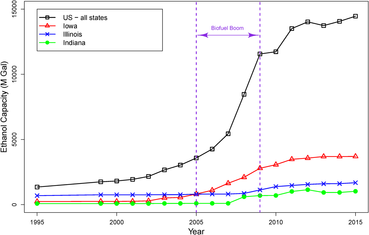
Figure 1. Ethanol Production Capacity in the United States and the Study Region (IA, IL, IN)
Figure 2 shows that the proportion of cropland in our study region (three Midwest states: IN, IL, IA) switching from regular <corn, soybean> rotation to continuous <corn, corn> production increased around the 2005–2009 biofuel boom. Figure A1 in the Appendix also presents the shares of three-period (<corn, corn, corn>) and four-period (<corn, corn, corn, corn>) corn monocropping, which show a similar trend. The rise of monocropping indicates that farmers appeared to respond relatively quickly to the expected upward shift in demand resulting from the policy shock (Wilson, Gibbons, and Ramsden Reference Wilson, Gibbons and Ramsden2003, Motamed, McPhail, and Williams Reference Motamed, McPhail and Williams2016).
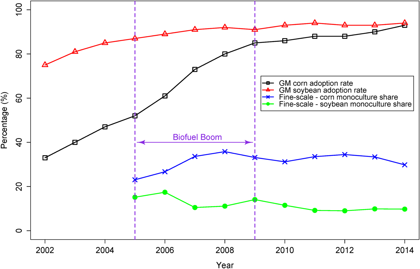
Figure 2. GM Crops Adoption Rate and Percentage of Fields Skipping Corn-Soybean Rotation
Overall, this study focuses on answering the following research questions: (1) Is the share of fields cultivated under corn monocropping responsive to price shocks reflected in the national crop commodity markets? and (2) Does the expansion in nearby ethanol production capacity have an impact on the propensity of engaging in corn monocropping? The empirical investigation in the study is based on a proportional response framework (Papke and Wooldridge Reference Papke and Wooldridge1996) to model the share of monocropping within each county in a panel data setting. The panel data consists of over 100 million land pixels at 30-meter resolution from 293 counties in the Midwest (IN, IL, and IA) with a study period of 2005–2014. In particular, we examine the time-varying economic drivers of crop rotational patterns while controlling for time-invariant factors through fixed effects. A key feature of our analysis is that we harness high-resolution remote sensing-based data on crop choice to analyze crop rotation patterns, which are typically unobservable to researchers and difficult to identify with aggregate county-level acreage data. Figure 3 illustrates the underlying land cover data for two subsequent years over a small area of the sample. The high level of detail allows us to characterize cropping decisions at the field level over time and across large areas, and to derive insights regarding the drivers underlying these regional patterns.
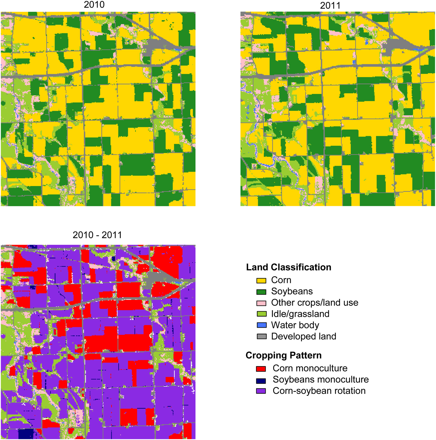
Figure 3. Land Classification and Rotation Patterns for a Small Area in the Sample
Most of the recent literature on crop rotations, especially in agronomy, focuses on the yield disadvantage of monocropping systems. In a multi-location field study, Porter et al. (Reference Porter, Lauer, Lueschen, Ford, Hoverstad, Oplinger and Crookston1997) find that, relative to continuous corn, corn rotated annually with soybeans yields 13% more, controlling for use of other inputs, and first-year corn following multiple years of soybean yields 15% more. The yield penalty from continuous corn can be as high as 25% in low-yielding environments (Porter et al. Reference Porter, Lauer, Lueschen, Ford, Hoverstad, Oplinger and Crookston1997). Among the major factors explaining this yield difference is the net soil nitrogen mineralization of soybean residues, which provides a yield boost to the following corn crop (Gentry, Ruffo, and Below Reference Gentry, Ruffo and Below2013). Similar evidence is found in Krupinsky et al. (Reference Krupinsky, Tanaka, Merrill, Liebig and Hanson2006).
Naturally, the choice that farmers make to engage in monocropping is an economic decision (Peter and Runge-Metzger Reference Peter and Runge-Metzger1994, Hennessy Reference Hennessy2006). For instance, a farmer may choose a continuous corn monocropping system over a regular <corn, soybeans> rotation if there is a premium on corn price that at least compensates for the lower average yield of the monocropping system. The premium could originate from a higher market price or from local demand for animal feed that is not directly observable to the researcher. While previous work has examined acreage response to price changes (e.g., Hendricks, Smith, and Sumner Reference Hendricks, Smith and Sumner2014a), we examine changes in the share of monocropping due to market fluctuations.
Our results indicate that there are both time-varying and time-invariant economic drivers in explaining farmers' decisions to skip regular crop rotations and engage in corn monocropping. For example, the panel data model results suggest that a $1.00/acre (2015 USD) increase in the return for corn is associated with a 0.015% increase in the percentage of fields skipping <corn, soybean> rotation and planting corn continuously. To put this in context, a one-standard-deviation increase in return for corn ($115.15/acre) implies a 1.73% increase in two-period corn monocropping. In addition, we find that a $1.00/acre (2015 USD) increase in the return for soybeans is associated with at least a 0.02% decrease in the proportion of two-period corn monocropping. To put this in context, a one-standard-deviation increase in return for soybeans ($73.16/acre) implies a 1.46% decrease in two-period corn monocropping. The results may be interpreted in other ways, such as from a perspective of yield change or a perspective of the change in the short-run probability of planting corn after corn. The implications of the findings are explored in the paper.
Method
Empirical Framework
We hypothesize that farmers tend to increase the share of monocropping when the expected market returns for crops rise, whereas they tend to decrease the share of monocropping when lower market returns are expected. Figure 4 conceptually illustrates the influence of relative returns of corn and soybeans on monocropping and rotations. A complete theoretical treatment of the dynamics of crop rotations and monocropping can be found in Hennessy (Reference Hennessy2006). Our empirical investigation focuses on quantifying how different drivers of crop returns affect the incidence of monocropping in the Midwest.
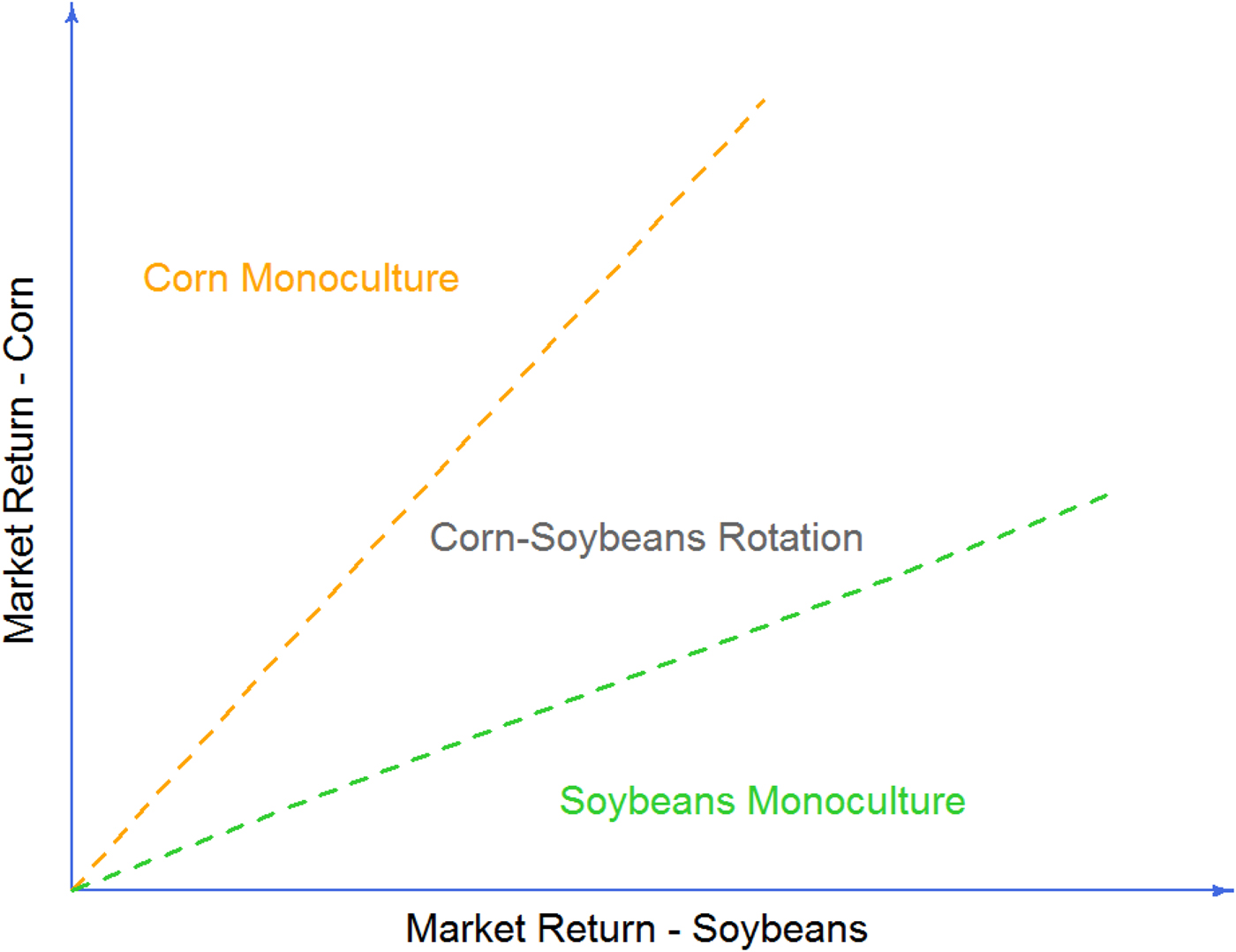
Figure 4. Market Return for Crops, Crop Rotation, and Monoculture
We consider both market-wide and local drivers of crop market returns. For instance, shocks to international trade and changes in biofuel policies can affect crop output prices differently. The market-wide changes are relatively easy to observe, as they vary over time. On the other hand, there are drivers that solely shift the relative returns of a crop in a particular locale. For instance, the presence of soils that are more suited for a given crop makes the crop relatively more profitable locally. So does the presence of local demand for the crop. For example, the demand for corn silage from nearby livestock production can make corn production more profitable in the long run. Similarly, the proximity to an ethanol plant can reduce transportation costs for corn, thus making its production more profitable in its vicinity. These local shifters of returns are more difficult to quantify.
More specifically, our empirical investigation explores both transitory and permanent drivers of crop returns affecting the spatial and temporal patterns of monocropping in the Midwest. We put particular emphasis on market-wide phenomena that shift the overall relative returns of corn and soybeans. We also explore the influence of the installation of ethanol plants as a potential time-varying local shifter. Finally, we explore the unexplained permanent drivers of monocropping.
We derive our empirical model from a binary discrete choice framework of crop rotation. Suppose a farmer can freely choose to grow two major crops (corn and soybeans), and in general, she chooses to follow a corn-soybean rotation under normal market conditions to maximize her utility. However, the farmer may choose to skip or “break” the rotation and adopt a monocropping system to take the advantage of changing market conditions. Suppose there are N fields, and the cropping decision on the i − th field in year t can be represented by the following latent model:
 $$ {\phi} _{it}^{\ast} = X_{it}\beta + \delta _i + \varepsilon _{it} $$
where X it is a matrix of variables which affect expected outcome  $ \phi _{it}^{\ast} $ (i.e., net utility or achievement from growing crops). δ i is a component unique to location i. εit is an idiosyncratic error associated with field i and year t, which is private knowledge and known to the farmer but unobservable to the researcher. The researcher does not observe $ \phi _{it}^{\ast} $, and can only observe the discrete choice $ \phi _{it} $ made by the farmer, which is based on the following rule:
 $$ \matrix{ {{\phi} _{it} = 1} & {if\; {\phi} _{it}^{\ast} \gt 0} \cr {{\phi} _{it} = 0} & {if\; {\phi} _{it}^{\ast} \le 0} \cr} $$
The above model represents the farmer's benefit-cost analysis of deciding to “break” the normal crop rotation if the net utility for doing so is positive. Since we cannot measure this net utility and what we can only observe is the actual decision that the farmer has made, the model in (1) and (2) cannot be estimated with usual linear regression methods. Instead, one can estimate a discrete choice model with a dependent variable representing the observable outcome  $ \phi _{it} $. One necessary assumption for this purpose is that εit is independently distributed with the logistic distribution (Maddala Reference Maddala1983). Given the assumption, it follows that:
 $$ \matrix{ {\Pr \lpar {\phi} _{it} = 1 \vert X\rpar } & \hskip-4.35pc= {\Pr \!\lpar {\phi} _{it}^{\ast} \gt 0 \vert X\rpar } \cr & \hskip+-.5pc= {\Pr \!\lpar X_{it}\beta + \delta _i + \varepsilon _{it} \gt 0 \vert X\rpar } \cr {} & \hskip-4.9pc= {F\lpar X_{it}\beta + \delta _i\rpar } \cr} $$
where  $ F\lpar \cdot \rpar $ is the cumulative distribution function (CDF) for a logistic variable. Using this conditional probability, we can construct a log-likelihood function to estimate β and δ i.
In this study, with high-resolution data, we have hundreds of millions of observations. The volume of data makes it very difficult to estimate the discrete choice model at the pixel level. A simple way to reduce the computational difficulty is to aggregate the data. In our case, given that the crop yield and price/cost data are observed at the county level, we aggregate the pixel-level choices to a county-level share of fields under monocropping. If there are M j pixels in a county j, then a new dependent variable Πjt can be defined as 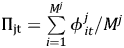 $ {\rm \Pi} _{{\rm jt}} = \mathop \sum \limits_{i = 1}^{M^j} \phi \,_{it}^j /M^j $. With the same binary response foundation, we can construct the logit (log-odds) at the county level directly. For county j, denoting odds of monocropping as Πjt/(1 – Πjt), taking log transformation yields logit(Πjt) = log(Πjt/(1 – Πjt)). Similar to the pixel-level binary logistic regression model, the goal is to model the log-odds of monocropping (skipping the rotation) as a function of explanatory variables X it and δ i. Now the regression model becomes:
 $$ {\rm logit}\lpar \Pi _{\,jt}\rpar \; = \log \displaystyle{{\Pi _{\,jt}} \over {1-\Pi _{\,jt}}} = X_{\,jt}\beta + \delta _j + \varepsilon _{\,jt} $$
Note that, if all the explanatory variables X are measured at the aggregated county level, then for a given county j, we have the same X it for all i = 1, …M j pixels in county j. In such a case, estimating an aggregated percentage/proportion model like the one in (4) and estimating a pixel-level binary logistic regression model based on the conditional probability defined in (3) should be equivalent, because both models rely on the same underlying set of information to identify β and δ j.
In our context, we rely on a panel model with fixed effects to estimate the contribution of time-varying drivers of returns of corn and soybeans to the county-level proportion of monocropping. This approach controls for unobserved heterogeneity. The estimation is computationally tractable given the relatively small number of counties compared to the number of fields underlying our county-level aggregates. In general, estimating a fixed effect logistic regression model is not an easy task in the presence of numerous cross-sectional units. Thus, the model is typically estimated relying on some sort of computational simplification, such as based on a conditional likelihood function (Chamberlain Reference Chamberlain1980).
More specifically, the estimation proceeds with a generalized linear model using the logit link function. The dependent variable is the proportion of <corn, corn> monocropping that is between 0 and 1. The proportion can be used to compute the odds ratio empirically. The log of the empirical odds ratio can be used as the dependent variable to estimate the model in equation (4) with a linear regression method, which is equivalent to the generalized linear model using the logit link function adopted in this study. The latter takes the proportion as the dependent variable directly. In the estimation, X consists of market return measures for each of the main crops (corn and soybeans) and measures of ethanol production capacity around each county. In the following subsections, we discuss data sources and how we construct the market return variables for each crop and the ethanol production capacity variable.
Data
The study region consists of three U.S. states located in the heart of the Corn Belt: Indiana (IN), Illinois (IL), and Iowa (IA). These are among the top five corn-producing states in the nation and accounted for about 40% of the U.S. corn production value in 2015.Footnote 2 The region has a landscape comprised of high-quality cropland. The country's two major commercial crops (corn and soybeans) make up more than 95% of the area of crop production in the region, making it an ideal area to study monocropping and crop rotations.
The crop choice data (NASS 2015) is derived from the USDA National Agricultural Statistics Service (NASS) Crop Data Layer (CDL). The CDL is a high-resolution remote-sensing land cover classification of the contiguous United States. The dataset is updated annually and has a 30-meter resolution for most years between 2001 and 2014, except for the 2006–2009 period for which the resolution was 56 meters. For these four years, we resampled data layers to 30 meters in ArcGIS 10 with the nearest neighbor algorithm, which is commonly used for discrete data such as land use classes (ESRI 2011). The 30-meter data pixels are small enough that six of them fit in a standard football field. We restrict the sample period to 2005–2014 to avoid relying on CDL data generated with a less accurate land cover classification algorithm that was discontinued in 2005 (Stern, Doraiswamy, and Akhmedov Reference Stern, Doraiswamy and Akhmedov2008, Johnson Reference Johnson2013).
The original CDL data provides more than 200 crop classification codes. In this study, we only focus on three types of them: corn, soybeans, and idle cropland (including grassland and pasture that can presumably be converted into crop production). These three types of land cover amount to more than 99% of all cropland in the study region. To facilitate the statistical analysis, we recoded the CDL data layers based on the rules specified in Table A1 in the Supplementary Appendix. Note that we exclude all pixels with double crops (< 0.01%), even if one of the two crops in a double-cropping system is either corn or soybeans.Footnote 3 Based on the re-classified data, we construct a large panel of 30-meter pixels. The panel is restricted to observations that are categorized as corn, soybeans, or idle in all sample years. The panel consists of about 165 million cross-sectional 30-meter pixels. To reduce the computational burden, we randomly sampled 10% of the data for the analysis.
We define crop rotation breaks in the following way. For a given pixel, if corn was grown the previous and current year, then we classify the case as a “break” from the traditional <corn, soybeans> rotation. If corn was grown the previous year and either soybeans or idle land is observed the current year, then the case does not constitute a break from the <corn, soybeans> rotation. In this study, we focus on corn monocropping, which is of greater interest given the recent market and policy context. The main empirical analysis focuses on two-period corn monocropping (<corn, corn>), but we also consider the case of three-period corn monocropping (<corn, corn, corn>). Results remain qualitatively similar. Given that the analysis incorporates information about the previous year in defining a rotation, the study period effectively used for estimation reduces to 2006–2014.
We compute the dependent variable of this study, the share of two-period corn monocropping, as the ratio of the total number of pixels growing corn both in the previous year and in the current year to the total number of corn pixels grown in the previous year. We subsample repeatedly from the pixel-level data and find that county-level ratios hover around 0.32 over the sample (see summary statistics in Table 1). The independent variables include mainly the expected crop returns and local ethanol production capacity.
Table 1. Summary Statistics

Note: All expected market return variables are measured in 2015 USD. The data sample includes 2,637 county-level observations and the study period ranges from 2005 to 2014.
Market Variables
To construct the expected market return variables for each crop, we collect data on crop yields, output prices, crop future prices, and production costs. The observed yield data used to generate expected crop yields were obtained from the USDA NASS (annual survey data). We obtain crop production costs and crop prices data from the USDA Economic Research Service (ERS), which is reported for ERS Farm Resource Regions. The future prices of corn and soybeans were obtained from TradingCharts.Footnote 4 When forecasting yields and prices, historical data of the extended time series from 2000 to 2014 are used.
We construct an expected net market return measure for each crop in the following way. For each year and field, a farmer expects to receive a location and time-specific net return from planting a given crop. Expectations on crop yield and output price are formed based on a time-series forecast. Denoting crop as s ∈ S = {corn, soybeans}, for county j in year t, the crop-specific expected yield is predicted as:
 $$ yield_{sjt} = \gamma _{sj} + \gamma _{s1}trend_{st} + \gamma _{s2}\,yield_{sjt-1} + \;e_{sjt} $$
where trend st captures the secular trend (e.g., technological progress) in crop yields. In this study, we use a linear time trend due to the relatively short sample period. γ sj is a time-invariant crop-specific county fixed effect, and e sjt represents a random shock to crop yield.
We construct expected crop prices in a similar way with an AR(1) process. A similar approach has been used in the literature (e.g., Coyle Reference Coyle1992, Scott Reference Scott2013, Haile, Kalkuhl, and von Braun Reference Haile, Kalkuhl and von Braun2014). Since crop price is usually determined at the regional level and does not vary much across counties, we drop the county dimension when forecasting. For crop s, its expected price for year t depends on a crop-specific constant, time trend, the price of last year, and the December crop future price on April 1 of the given year:
 $$price_{st}\; = {\phi} _{s0} + {\phi} _{s1}trend_{st} + {\phi} _{s2}price_{st-1} + {\phi} _{s3}Decprice_{st} + \;e_{st}$$
Given the expected yield and price above, and denoting production cost per acre as cost st, we can compute a crop-specific expected net market return (r) as the following:
 $$r_{sjt}\; = yield_{sjt} \times price_{st}-\;cost_{st}$$
For crop production costs, we use the current-year cost estimates from the ERS data directly, which is also reported for the ERS Farm Resource Regions. The main reason is that farmers very likely observe the input costs before making their planting decisions. Hence, there is no need to predict the production cost using historical data. Based on the regional ERS data, the coefficient of variation of the price ratio between corn and soybeans is about two times the coefficient of variation of the operating cost ratio. In other words, most of the variation in market return for a crop comes from output price variation, and less comes from changes in input prices. In addition, input costs appear to be fairly predictable given their relatively low variability. Similar to the output price information, the cost data is also provided at the regional level. This means that the unobserved local cost drivers are not captured by this variable. However, if these drivers are time-invariant they will be captured in the county fixed effects. Given the setup in (4) and (7), the main estimation equation can be written as:
 $$ {\rm logit}\lpar \hat{\Pi} _{\,jt}\rpar \; = \beta _1r_{\,jt\comma corn} + \beta _2r_{\,jt\comma soybean} + ethanol_{\,jt} + \delta _j + \varepsilon _{\,jt} $$
where  $ { \hat{\Pi}} _{\rm j} $ indicates that we do not observe the odds ratio directly. Instead, we compute the odds ratio empirically using the observed percentage of two-period corn monocropping in each county. In the results and discussion section, we focus on equation (8), which is estimated as a panel data model. Note that an implicit assumption in the empirical model is that variances and covariance of crop returns are time-invariant and being absorbed into fixed effects δ j. We only maintain this assumption due to data limitations. If spatially finer data on crop returns were available, measures on variances and covariance of crop returns could be included in the empirical model.
Ethanol Production Capacity
Data on ethanol production capacity and plant location were compiled from Ethanol Producer Magazine and from reports by the Renewable Fuels Association.Footnote 5 As of January 1, 2016, and according to the U.S. Energy Information Administration (EIA), there were 195 active ethanol plants in the United States. In 2016, the total nameplate ethanol production capacity reached almost 15,000 Mgal/year.Footnote 6 We expect that the increase in the ethanol production capacity around a given county would increase the propensities of corn monocropping through the price channel (Carter, Rausser, and Smith Reference Carter, Rausser and Smith2017). Normally, the location decision of an ethanol plant is made at the regional level and may be affected by other policy factors. Therefore, it is reasonable to consider the ethanol production capacity around a given county being exogenous to a farmer's crop choice decisions at the field level.
In this study, we measure the presence of ethanol production in two ways. The first metric is a dummy variable indicating whether there is a new ethanol plant within 30 miles of the county geographic center. The variable aims to capture recent changes in the local demand for corn that could be visible to farmers in a given county. The second metric is a measure of ethanol production capacity-weighted by the geographic distance from the country centroid to ethanol plants. More specifically, we define the weighted ethanol capacity measure as:
 $$ Ethanol_j\; = \sum\limits_{k = 1}^{K_j} {c_k\lpar 1-\displaystyle{{dist_{\,jk}} \over {range}}\rpar } $$
where K j is the total number of ethanol plants within a given radius (defined by range, which is set at 400 miles in this study) of county j, and dist jk denotes the distance from the geographic center of county j to ethanol plant k. c k is the capacity of plant k. Because there is new construction as well as changes in the ethanol production capacity over time, this variable is time-varying.
Results and Discussion
Main Findings
We first consider a basic model to assess how the cross-sectional variation in market returns affects the proportion of two-period corn monocropping across the sample region. For this purpose, we average all variables over time to estimate a “between-county” cross-sectional model of proportions of corn monocropping regressed on expected returns of corn and soybeans and weighted ethanol production capacity. The cross-sectional variation can be interpreted as the steady state of corn monocropping in the study region. The empirical results are reported in Table 2 for specifications exploiting sample-wide, within-state, and within-district variations.
Table 2. Model Coefficient Estimates with the Cross-Sectional Data
Note: (1) Throughout the paper, asterisks (*, **, ***) indicate statistical significance at the 10%, 5%, and 1% level, respectively, unless otherwise noted. (2) The level of significance is indicated based on Huber-White robust standard error.
We find that higher expected market returns for corn appear to be significantly associated with higher proportions of corn monocropping in both the sample-wide and within-state specifications (columns 1–2, Table 2). Similarly, a higher expected return for soybeans decreases the proportion of corn monocropping. Because most of the cross-sectional variation in returns stems from relative differences between corn and soybean yields, the result suggests that areas with more favorable conditions for corn (relative to soybeans) tend to exhibit a greater rate of corn monocropping. Note that the coefficients for the within-district specification remain insignificant (column 3, Table 2), which may signal there is insufficient variation within each of the 27 districts for a proper estimation given the small cross-sectional sample of 293 counties. Notice that the effect of ethanol production capacity is only significant in the within-state model (column 2, Table 2), with an expected positive sign. This result indicates that there is a positive association between the incidence of corn monocropping and the presence of ethanol production capacity. Table A2 in the Supplementary Appendix shows that these cross-sectional results remain qualitatively similar when we consider the three-period corn monocropping.
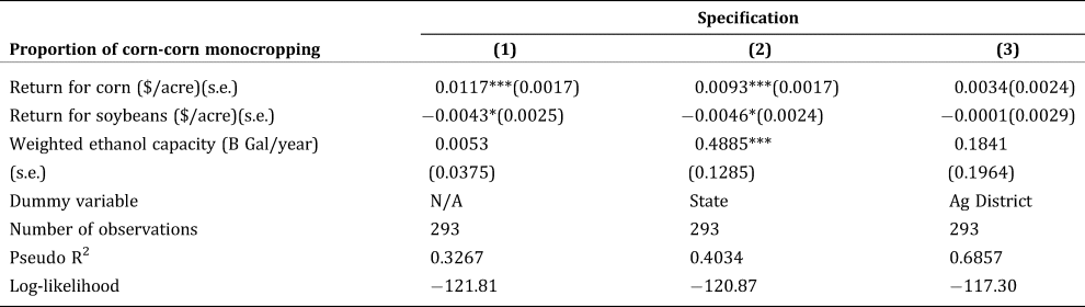
Moving to the county-level panel data model, Table 3 shows that expected crop returns constitute a key driver for engaging in corn monocropping. This table shows that coefficient signs are theoretically consistent and robust to different specifications. Somewhat surprisingly, in the fixed effects panel data model, nearby ethanol production capacity does not appear to influence the proportion of corn monocropping, regardless of the nature of the ethanol production variable used (weighted ethanol production capacity or new plant dummy). This result indicates that ethanol production capacity does not seem to influence crop rotation decisions at the county level. One possible explanation is that transportation costs are low enough that the proximity to ethanol production does not constitute a strong enough shift in the local demand to justify skipping traditional rotations.
Table 3. Model Coefficient Estimates with the Panel Data
Note: The standard error estimates are based on Huber-White robust standard error.
The panel data estimation is based on a generalized linear regression model with the logit link function, and therefore the parameter estimates do not have the familiar interpretation as marginal effects directly. In our case, the marginal effects are conditional on the level of the variables, so we need to specify a given level when reporting the marginal effects. For this purpose, we treat all dummy independent variables as balanced and select the mean value for continuous variables such as expected market return or ethanol production capacity.
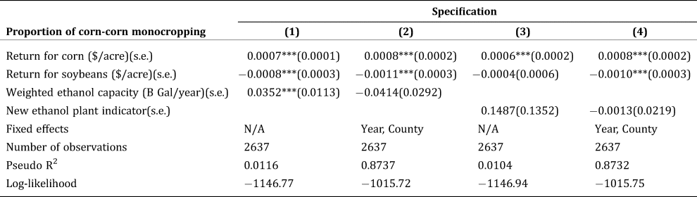
Estimated marginal effects are presented in Table 4 for three different specifications. The marginal effect of expected corn return on the proportion of two-period corn monocropping is 0.0019 for the cross-sectional model with state dummy variables (column 1). This implies that an increase of $1.00/acre (2015 USD) in return for corn can increase the fields skipping <corn, soybean> rotation and planting corn continuously by 0.19%.Footnote 7
Table 4. Marginal Effect Estimates from the Cross-Sectional and Panel Data Models
Note: The standard errors for marginal effects are computed using the Delta method.
On the other hand, the marginal effect estimate of -0.0009 for expected soybeans return implies that a $1.00/acre (2015 USD) increase in return for soybeans can decrease the fields skipping <corn, soybean> rotation by 0.09%. Recall that in the cross-sectional model, the variation in explanatory variables is driven by the cross-sectional variation of crop yields in the long run. Thus, one can interpret this result in light of spatial yield differentials. For instance, a one-standard-deviation increase in corn yield (8.77 bushels/acre, in the cross-sectional data) is associated with a 6.67% increase in corn monocropping holding the price of corn at $4/bushel and the production cost unchanged. In addition, an estimate of 0.1012 for weighted ethanol production capacity suggests that an expansion of 98.8M gallons in nearby ethanol production capacity, the equivalent of a medium-sized plant, would be associated with a one-percent increase in fields engaging in two-period corn monocropping. This illustrates how small the estimated impact of nearby ethanol production capacity is on corn monocropping even in the long run. This is consistent with the recent literature showing that crop price is a much more important driver of acreage response compared to nearby ethanol production capacity (Li, Miao, and Khanna Reference Li, Miao and Khanna2018).
The interpretation of coefficients for the panel data model specifications with county fixed effects (column 2 and 3, Table 4) is similar, but we are exploring the “within” county variations. A marginal effect of 0.00015 for corn return implies that a $1.00/acre (2015 USD) increase in the expected return for corn can on average increase the fields engaging in two-period corn monocropping by 0.015%. To put this in context, the annual change of expected return for corn ranges from $−356.88 to $352.77/acre during the sample period. Thus, the highest rate of change observed in the data ($352.77/acre) implies an increase of 5.35% in fields engaging in two-period corn monocropping. This result is consistent with the overall pattern observed in the aggregate CDL data (see Figure 2).
Similarly, a marginal effect of -0.00021 for soybeans implies that a $1.00/acre (2015 USD) increase in the expected return for soybeans is on average associated with a 0.021% reduction of fields engaging in two-period corn monocropping. Again, to put this in context, the annual change of expected return for soybeans ranges from $−225.31.96 to $217.02/acre during the sample period. The highest rate of change observed in the data ($217.02/acre) would imply a decrease of 4.56% in fields engaging in two-period corn monocropping. In a nutshell, the price fluctuations of the two main crops have counterbalancing effects on the proportion of corn monocropping in the short run.
Hendricks et al. (Reference Hendricks, Sinnathamby, Douglas-Mankin, Smith, Sumner and Earnhart2014b) offer an alternative way to interpret the estimated marginal effects: estimating the change in the probability of continuous corn due to price change using Markov transition probabilities. The estimated marginal effects in this study are effectively one of the transition probabilities—the probability of planting corn conditional on having planted corn the previous year. Following Hendricks et al. (Reference Hendricks, Sinnathamby, Douglas-Mankin, Smith, Sumner and Earnhart2014b), multiplying the estimated marginal effect with the long-run probability of planting corn gives the short-run change in the probability of planting corn after corn. During the ten years of the study period, on average 56.26% of the fields were planted with corn, which can be used to approximate the long-run probability of planting corn. Therefore, the estimated marginal effect of 0.00015 for corn return implies that a $1.00/acre (2015 USD) increase in the expected return for corn can increase the short-run probability of planting corn after corn by 0.0084%. That is, a one-standard-deviation increase of return for corn ($115.15/acre) can increase the short-run probability of planting corn after corn by almost one percent.
Unexplained Time-Invariant Drivers
So far we have discussed variation in corn monocropping that we can attribute to cross-sectional or temporal variation in the explanatory variables. It is possible, however, to visualize the unexplained variation about the time-invariant propensity of two-period corn monocropping. To do so, we represent the county fixed effects of the proportional panel model in units of the dependent variable (Figure 5). These fixed effects are conditional on the market-level factors at play and embody the unexplained time-invariant variation in two-period corn monocropping in the sample. It is clear from the map that certain regions, such as counties in northern Illinois and northeastern Iowa, have higher propensities of corn monocropping.
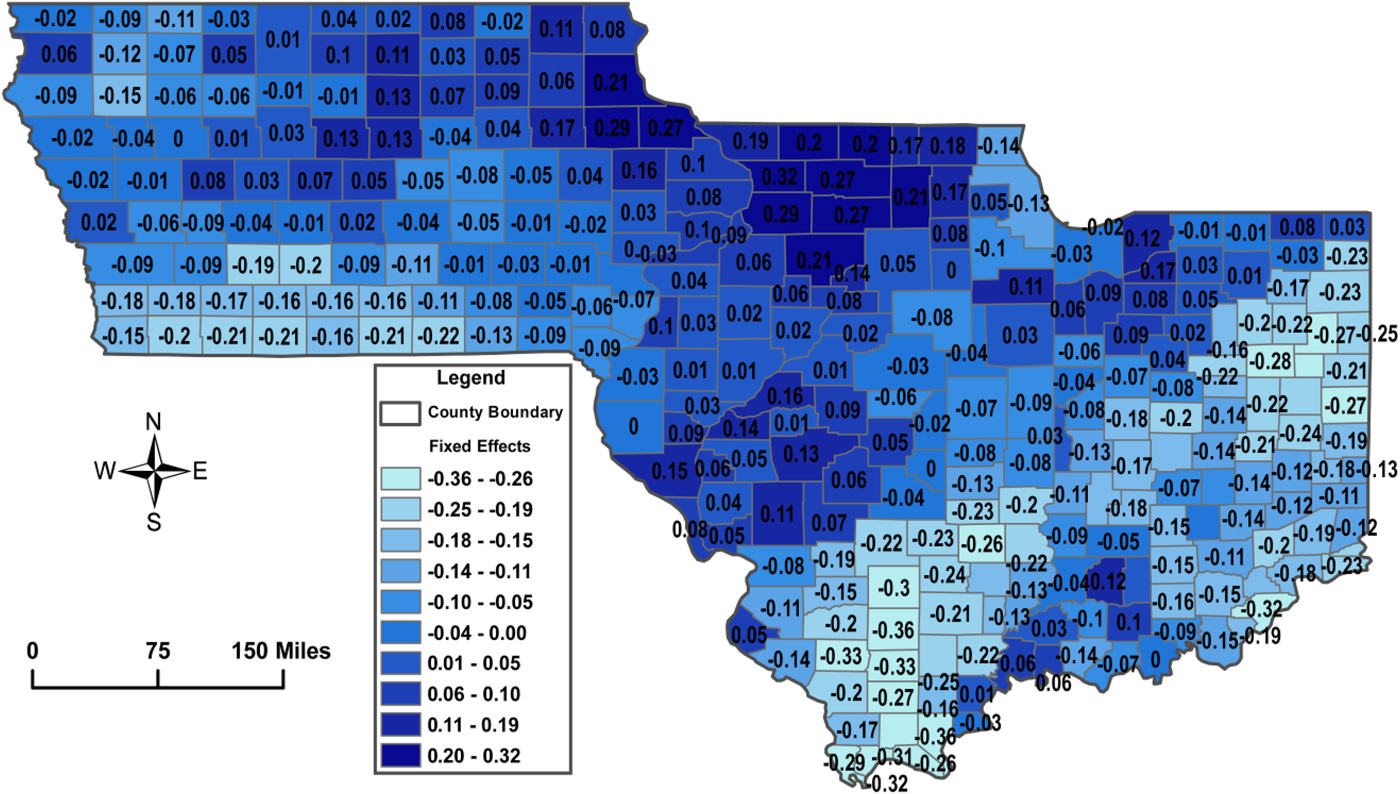
Figure 5. Time-Invariant Share of Corn Monocropping Based On Estimated County Fixed Effects
Genetically Modified (GM) Crops
It is worth noting that monocropping has been anecdotally linked to the advent of biotechnology and more particularly to the rise of GM crops. Since the mid-1990s, biotechnology development has enabled the introduction of crops with genes that confer valuable traits to farmers such as the resistance to pests and weeds. These GM crops appear to be more beneficial to farmers given their relatively rapid and widespread adoption to the detriment of non-GM crops (Fernandez-Cornejo et al. Reference Fernandez-Cornejo, Wechsler, Livingston and Mitchell2014). While serious social and ecological concerns have been raised regarding GM crops (e.g., Dale Reference Dale2002, Cellini et al. Reference Cellini, Chesson, Colquhoun, Constable, Davies, Engel, Gatehouse, Kärenlampi, Kok, Leguay and Lehesranta2004), there have been substantial net economic benefits to farmers amounting to $27 billion between 1996 and 2006 across the globe (Brookes and Barfoot Reference Brookes and Barfoot2006). GM technology also seems to have reduced pesticide use, with some potential benefits to the environment (Ammann Reference Ammann2005). Aside from its potential adverse effects on human health, animal health, and the environment (e.g., Cellini et al. Reference Cellini, Chesson, Colquhoun, Constable, Davies, Engel, Gatehouse, Kärenlampi, Kok, Leguay and Lehesranta2004), a lingering question is to what extent GM technology has altered the conventional crop rotation system.
In principle, GM technology provides benefits that could explain the rise of monocropping. For instance, using experimental data from ten U.S. university extension services, Nolan and Santos (Reference Nolan and Santos2012) find that GM traits tend to increase crop yields, controlling for other factors, with the yield boost varying by crop and the stacking of GM traits in a single crop. However, much of the existing literature has paid little attention to the effect that GM technology may have on the cropping systems. Figure 1 illustrates that the adoption of GM corn has spread rapidly across corn-growing regions over the last two decades. However, this pattern does not coincide with the evolution in the proportion of fields that we have identified as skipping the <corn, soybean> rotation in our sample. This suggests that traditional rotations appear, at first glance, to be operating in “business as usual,” except during the price shock resulting from the biofuels blending mandate introduced in the Energy Policy Act of 2005 (see footnote 1). In other words, there may be little connection between the rate of GM crop adoption and the prevalence of monocropping. One possible explanation is that the adoption of GM crops does not substitute for the benefits of traditional crop rotations, so that biotechnology and conventional rotations provide complementary benefits.
Conclusions
In this study, we develop an empirical model to examine the economic drivers of corn monocropping in the U.S. Midwest. We rely on a combination of data sources that include high-resolution remote-sensing land cover data over the past decade. The proposed empirical model allows us to study the effects of market-wide and local factors that affect the propensity of continuous corn monocropping.
We identify time-varying and potential time-invariant factors that play an important role in influencing farmers' decisions about following or skipping regular crop rotations. For example, we find that a $1.00/acre (2015 USD) increase in the expected return for corn can on average increase the percentage of fields engaging in two-period corn monocropping by 0.015%. Given that our dependent variable is effectively a transition probability that represents the county-level likelihood of planting corn conditional on having corn planted the previous year, the marginal effect estimate can also be interpreted as that a $1.00/acre (2015 USD) increase in the return for corn can increase the short-run probability of planting corn after corn by 0.0084%. That is, a one-standard-deviation increase of return for corn ($115.15/acre) can increase the short-run probability of planting corn after corn by roughly one percent. We find that these estimates are in the order of magnitude that would explain the observed increase of corn monocropping in the Midwest (IN, IL, and IA) during the 2005–2009 biofuel boom.
In addition, we find a tenuous cross-sectional association between the nearby presence of ethanol production and corn monocropping. However, this association vanishes as we explore the within-county temporal variation. We also find suggestive evidence that GM crop adoption for both corn and soybeans do not seem related to the likelihood of monocropping adoption. Finally, we explore the spatial and time-invariant variation in corn monocropping at the county level. Future research could help identify explicitly the drivers of the cross-sectional variation that remains unexplained in this study. We suggest that local factors such as livestock production clustering, soil quality, topography, and farmer characteristics could be at play and may be explored with more detailed data. This study illustrates the promising use of high-resolution remote-sensing data to tackle important agribusiness and agro-environmental policy questions that remain elusive with aggregate data.
Supplementary material
The supplementary material for this article can be found at https://doi.org/10.1017/age.2019.4


 Open access