


1. Introduction
The loss of labor and know-how of productive adults due to diseases highly reduces the productivity of agricultural labor in developing countries (World Bank 2008). In Burkina Faso, desertions of labor due to illnesses are more frequent in the rainy season. Yet the foundation of agricultural production is pluvial and depends on the availability and quality of labor that is unfortunately affected by health and disease shocks. Because of the lack of prevention programs and efficient health care throughout the country, diseases considerably affect the productivity of farming labor.
With a gross mortality rate of 11.8 percent in 2006 and a life expectancy of 57 years in 2008, the health issue remains quite concerning, especially for rural populations. The epidemiological profile is characterized by the persistence of a high morbidity rate due mainly to malaria, respiratory infections, malnutrition, diarrheic diseases, and HIV/AIDS (Ministère de la santéFootnote 1, 2011). These different diseases affect the productivity of rural households’ agricultural labor. However, without a significant gain in farm labor productivity, it is hard to sustain hunger and poverty alleviation (Timmer Reference Timmer2008).
To reduce the incidence of disease in rural areas, health policy has focused on the supply of primary health care since 2000. The budget allocated to the health sector has increased from 7.07 percent in 2000 to 15.46 percent in 2009. The average coverage of a health and social promotion center (HSPC) decreased from 9.38 km in 2000 to 7.34 km in 2010 (Ministère de la santéFootnote 2 2010). In spite of this tangible improvement of the rural households’ access to primary health care, Burkina Faso has still not achieved the Bamako InitiativeFootnote 3 goals that recommend a maximal coverage of 5 km per health facility.
After more than a decade of efforts in improving the access of rural households to health services, there is almost no research evaluating the effects of the use of health services on farm labor productivity in Burkina Faso. Nevertheless, this question is of great interest for this country, where almost 80 percent of the population lives in rural areas and depends on agriculture for their livelihood (Savadogo et al. Reference Savadogo, Bambio, Combary, Ouédraogo, Sawadogo, Tiemtore and Zahonogo2011). The poverty profile indicates that most rural households live below the poverty line (Ministère de l'Economie et des FinancesFootnote 4 2010).
Despite the theoretical agreement about health effects on agricultural labor, the results of empirical studies are quite divergent and sometimes contradictory. Poor health can have negative effects on labour productivity by reducing physical and cognitive capacities and working time. These results were found by Touzé and Ventelou (Reference Touzé and Ventelou2002) and Perkins, Radelet, and Lindauer (Reference Perkins, Radelet and Lindauer2008). However, public health expenditures by the state for the benefit of the population may have a positive effect on agricultural labour productivity. This has been shown by Fan and Hazell (Reference Fan and Hazell1999); Fan, Zhang, and Zhang (Reference Fan, Zhang and Zhang2002); Fan and Thorat (Reference Fan and Thorat2003); Rivera and Currais (Reference Rivera and Currais2003); Pham, Minh, and Duong (Reference Pham, Minh and Duong2006); Hassan (Reference Hassan2008); and Karbasi and Mojarad (Reference Karbasi and Mojarad2008).
The divergences of these results are essentially explained by the existence of the selection bias that limits the identification of the real effect of health on the productivity of farming labor. Due to the lack of randomized data, most of these studies have used the matching method through the scores of propensity, the method of double differences, and the method of standard instrumental variables to solve the issue of selection bias. Yet none of these methods is even able to appropriately treat the problem of non-complier. Imbens and Angrist (Reference Imbens and Angrist1994) have shown that the local average treatment effect (LATE) estimator can correct both the problems of selection bias and non-complier.
In the context of this study, we make use of the instrumental variables method with an estimator LATE to assess the impact of the use of health services on the productivity of agricultural labor in cases of unexpected diseases during the rainy season. For this purpose, the distance from the household's homestead to the Health and Social Promotion Center (HSPC) has been considered as an instrumental variable. Thornton (Reference Thornton2008) used the distance from the HIV test results centers as an instrumental variable in the analysis of the effects of knowing HIV test results on condom purchase.
Burkina Faso's public health system is characterized by a pyramidal organization with four levels. The health and social promotion center (HSPC) represents the first level of care or first contact and is the one found in rural areas. In the case of care that cannot be provided by the HSPC, the first level of referral is the Medical Center with Surgical Antenna (MCSA). The second level of reference is the Regional Hospital Centers (RHC), and the last level of reference is the University Hospital Centers (UHC). In parallel with public health care institutions, a private offer has developed. As mentioned above, in Burkina Faso, the HSPC is the reference for health coverage policy in rural zones. Rural households must first go through the primary health centers, before accessing higher-level health centers. The traveling distance of a household to access the health center is the main criterion for the implementation of HSPC in rural zones. According to the Bamako Initiative launched in 1987 during an international conference on access to primary health care for all, a household has access to a health center when the distance from its homestead to the health center does not exceed 5 km.
It is plausible that the nearer the health center, the more likely households will attend a HSPC upon occurrence of a disease, because their transportation is easier and less costly. The variable distance of the household's homestead from a HSPC may therefore influence the decision of households to attend a health center in case of disease occurrence. However, this variable has a high probability not to be related to the agricultural productivity of rural households. The distance to a HSPC can therefore be used as an instrumental variable in the analysis of the impact of using HSPC on agricultural labor productivity. A validity test of this instrumental variable is carried out in the continuation of the article.
The article is divided into five parts. The first part was the Introduction. The second part presents the literature review and the theoretical model of the impact assessment. The third part explains the analysis method and presents the data. The fourth part provides the empirical results on the effects of health services on farm labor productivity. Finally, the fifth part draws conclusions and explanations of the study in terms of economic policies.
2. Modeling of the Effects of the Use of Health Services on Farm Labor Productivity
This section presents the literature review of the effects of the farmers’ state of health on agricultural productivity and the theoretical basis of the impact assessment on public policy.
2.1. Effects of Farmers’ Health on Agricultural Labor Productivity
Empirical results on the effects of the state of health on agricultural labor productivity are quite divergent. In mixed crops systems, Cole (Reference Cole, Hawkes and Ruel2006) noticed that the great majority of producers suffer from an intense muscular fatigue, exhaustion with sweat, and skin infection. This state leads to a decrease of agricultural productivity because of the accumulation of days of rest. According to Pitt and Rosenzweig (Reference Pitt, Rosenzweig, Singh, Squire and Strauss1986), diseases affecting younger children and old people diverts farming labor towards taking care of sick people, which contributes to the decrease of agricultural yields.
In a study carried out in Cameroon, Audibert (Reference Audibert1986) found that an increase of 10 percent of the prevalence of schistosomiasis reduces rice-growing production by 4.9 percent, while malaria has no significant effect. Audibert and Etard (Reference Audibert and Etard1998), in a similar analysis in Mali, found that health improvement has no effect on rice production, but it modifies the division of labor for different activities.
Meanwhile, in an quasi-experimental study in an irrigated rice-growing site affected by schistosomiasis in Mali, Audibert and Etard (Reference Audibert and Etard2003) observed a 26 percent production increase per man-day of family labor following health status improvement. In the same way, Audibert, Mathonnat, and Henry (Reference Audibert, Mathonnat and Henry2003) noticed that malaria had a negative effect on the technical efficacy of cotton production in Côte d'Ivoire. However, Audibert et al. (Reference Audibert, Brun, Mathonnat and Henry2009) did not observe a significant effect of malaria infection on coffee and cocoa production in Côte d'Ivoire.
Strauss (Reference Strauss1986) revealed that caloric contribution has a significant effect on the productivity of farming labor in Sierra Leone. Croppenstedt and Muller (Reference Croppenstedt and Muller2000) found a similar result in Ethiopia by displaying a significant link between health, nutritional status, and agricultural productivity. Meanwhile, Deolalikar (Reference Deolalikar1988) obtained different results when using panel data on regions in India.
Spear (Reference Spear1991) found that extended exposure to pesticides significantly hinders the farmers’ ability to work and contributes to a reduction in their management and supervision abilities. In the same way, Antle and Pingali (Reference Antle and Pingali1994) noticed that the use of pesticides in rice-growing in the Philippines had a negative effect on the farmers’ health status, while farmers’ health had a significant positive effect on rice productivity.
Baldwin and Weisbrod (Reference Baldwin and Weisbrod1974) showed that parasitic infections caused significant undesirable effects on the productivity of farming labor. These results were confirmed years later by Weisbrod and Helminiak (Reference Weisbrod and Helminiak1977). Meanwhile, Gilgen, Mascie-Taylor, and Rosetta (Reference Gilgen, Mascie-Taylor and Rosetta2001) did not find any significant difference in work productivity when treating vermifuge of adult tea gatherers in Bangladesh. Their results have nevertheless shown that anemia affects the amount of time worked and the productivity of agricultural labor.
Kim, Tandon, and Hailu (Reference Kim, Tandon and Hailu1997) analyzed the impact of disease on the productivity of coffee planting in Ethiopia. Their results revealed that the daily wages of employees affected by cutaneous problems were reduced by 10 to 15 percent. In Kenya's tea plantations, Fox et al. (Reference Fox, Rosen, MacLeod, Wasunna, Bii, Foglia and Simon2004) noticed that seropositive workers gathered less during the last two years of their lives: between 4.11 and 7.93 kg / day.
The works of Ulimwengu (Reference Ulimwengu2009) and Badiane and Ulimwengu (Reference Badiane and Ulimwengu2009) made use of regression techniques of the stochastic frontier method to evaluate the impact of farmers’ state of health on agricultural productivity in Ethiopia and Uganda, respectively. Their results displayed positive significant effects of health measures on the technical efficiency of agricultural production. In the case of Nigeria, Ajani and Ugwu (Reference Ajani and Ugwu2008) showed that the improvement of a farmer's health status leads to an increase of his efficiency by 31 percent.
2.2. Theoretical Model of the Impact of Evaluation of Health Services on Agricultural Productivity
According to human capital theory, men invest in health care, education, food, and migration for profit and nonprofit gains that they can draw on in the short and long term (Schultz, Reference Schultz1961; Becker, Reference Becker1964). The theoretical model of reference in terms of impact assessment of public policies has been implemented by Rubin (Reference Rubin1974). It leans upon the basic hypothesis of a lack of distribution of the treatment effect (T) within the population. The approach of the current study consists in measuring the impact of the use of health services (T i) on rural households’ farm labor productivity (Y i) in case of an unexpected disease. There are two potential results that cannot be observed simultaneously for the same rural household, Y 1i if the rural household has used health services (T i = 1) and Y 0i otherwise (T i = 0). For a household that has used health services, the result Y 0i corresponds to the counterfactual result (i.e., that which might have been carried out if it had not used health services).
The farm labor productivity observed at the level of each rural household i can be deduced from the relationship:

with N being the number of households where only the couple (Y i, T i) is being observed for each household.
The impact of the use of health services on the agricultural labor productivity of each rural household is measured by:

The variable of interest Δi is individual and unobservable; this renders its distribution in the population unidentifiable. However, by building a comparison group of households being able to reproduce the counterfactual result of the group of treated households and under some hypotheses on the triple joint (Y 0i, Y 1i, T i), it is possible to identify some parameters of the distribution Δi from the density of observable variables (Y i, T i).
The parameter of interest of this study is ΔTT, which represents the average effect of the use of health services on the rural households’ agricultural work productivity:

Under the hypothesis of independence between the potential results (Y 0i, Y 1i) and the variable of treatment T i, it is possible to write:


ΔTT being estimated as the difference of the means of agricultural productivity between the group of treated households and the group of control households. This result comes from the fact that the mean productivity of household agricultural labor that used health center services might have been the same as it would be had they not resorted to health center services:

If the independence hypothesis between the potential results and the treatment is not tested, that is,E(Y 0i|T i = 1) ≠ E(Y 0i|T i = 0), then the estimator ΔTT would be affected by one selection bias:

Where B TT represents the selection bias:

The selection bias comes from the fact that the mean counterfactual result of households having made use of health services might have not been the same as the one of households that have not used health services, in the absence of treatment. This is because the group of control households is not identical to the group of treated households. To solve this problem, it is necessary to adopt an approach that helps to reduce the possibility of selection bias.
3. Strategy for Identifying the Impact of Health Services on Agricultural Labor Productivity
The elimination of the selection bias and the treatment of non-complier form is the main concern of every impact assessment. Indeed, the main groups are defined according to their assignment to take the treatment (or not). Individuals in the control group should not receive treatment and individuals in the treatment group should receive treatment. This form of contamination is called “imperfect compliance.” “Compliers” always follow the assigned treatment: they will only take the treatment when they are assigned to take it and do not take the treatment when they are not assigned to take it. A certain group is made up of people who always take the treatment, whether they are assigned or not. Another group is made up of people who never take the treatment, whether they are assigned or not. We also have defiers who will always do the opposite: when they are assigned, they do not take the treatment and when they are not assigned, they take it. The comparison between those who take the treatment and those who do not, does not always provide a causal estimate of the effect of the treatment, since the reasons for imperfect compliance may well be correlated with other characteristics that affect the outcome. The instrumental variable method offers an econometric solution to assess the impact of a treatment even when there is “imperfect compliance.” The IV analysis provides a clear set of hypotheses to identify the effect of treatment for the sub-population of those who are compliant with treatment—the Local Average Treatment Effect (LATE)—i.e., compliers. The corresponding treatment effects for non-compliers (i.e., those who always take, those who never take, and defiers) are not identified (Angrist, Imbens, and Rubin Reference Angrist, Imbens and Rubin1996). The “Treatment on treated” estimator used here estimates the effect of offering and receiving treatment and thus corrects for the non-compliers problem. To deal with these questions, the study has used a strong and valid instrumental variable to estimate a LATE, has defined relevant variables, and has carried out tests of differences on the observable characteristics between the treatment and the control. This test ensures that the two groups are statistically identical and that randomization was done correctly. The least squares method does not offer an econometric solution for non-compliers problem.
3.1. The Instrumental Variables Method
The standard instrumental variables method enables elimination of selection bias and deals with the problem of treatment endogeneity (Heckman and Vytlacyl Reference Heckman and Vytlacil2000; Heckman and Vytlacyl Reference Heckman and Vytlacil2005; Heckman and Robb, Reference Heckman and Robb1985). The method assumes the existence of at least one instrumental variable that explains the treatment but has no direct effect on the result once the observable characteristics have been controlled. To assess the effects of the use of health services on farm labor productivity, we formulated the following model:

where Y i represents agricultural labor productivity.
T i represents the treatment variable that takes the value of 1 for the group of treated households and 0 otherwise.
X i is a vector of control variables.
The parameter of interest β 1 measures the impact of the use of health services on agricultural labor productivity.
The decision to use health services can be correlated with the observed or unobserved characteristics. So to correct the potential selection bias, we estimated in the first stage with:

where Z i represents the instrumental variable.
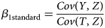
The standard parameter of interest is defined as:
If early unobserved gains of the use of health services affect the decision of resorting to the services of health centers in case of an unexpected illness, the standard estimator would be biased. To solve this problem, Imbens and Angrist (Reference Imbens and Angrist1994) developed the local average treatment effect (LATE) estimator. It measures the effect of the use of health services on agricultural labor productivity but only for households for which the change of the instrument has an effect on the decision of using health services (compliers). Under the hypothesis of monotonicity and the absence of non-compliers, it is possible to determine the size of compliers.
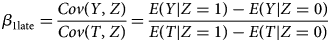
If the treatment and the instrument are binary variables, Wald's estimator can be used to estimate the LATE:
The method of estimation in two stages has been used to estimate the effect of the use of health services on agricultural labor productivity in case of an unexpected illness in the rainy season. In this article, the dependent variable is continuous and the treatment variable is binary. This requires that the endogeneity of the treatment variable be controlled. It is true that in this case, one could be tempted to use the 2sls method, but it is not appropriate because it leads to inconsistent estimators, as indicated by Wooldridge (Reference Wooldridge2010). The “treatreg” command found in the stata module takes into account the effects of the binary endogenous variable on the outcome of interest. It estimates the two regressions and yields robust standard errors. The “treatreg” command using a two-step consistent estimator is used in this paper. The two-step option specifies that two-step consistent estimates of the parameters, standard errors, and covariance matrix be produced.
To test the validity of the instruments, we use the Hausman (Reference Hausman1978) specification test to check for over-identification restrictions only for the standard IV model because the IV LATE is exactly identified. The Hausman specification test compares the estimators of the two models: the first estimator is the one of the LATE model which is just-identified because it has only one instrumental variable. The second estimator is relative to the standard IV model which is over-identified because it has two instrumental variables. The estimator of the just-identified model is considered to be consistent and the estimator of the over-identified model is considered to be efficient under the tested hypothesis. The null hypothesis is that the estimator of the over-identified model is indeed an efficient (and consistent) estimator of the true parameters. If this is the case, there should be no systematic difference between the two estimators. If there is a systematic difference between the estimates, then one may question the assumptions on which the efficient estimator is based.
3.2. Presentation of the Study Data
This section presents the source and method of data collection, defines the model's variables, and gives a descriptive analysis of farmer characteristics data.
3.2.1. Source and Method of Data Collection
Data collection was carried out through the “Convergence” project, a project conducted by the Laboratory of Quantitative Analysis Applied to Development – Sahel (LAQAD-S) in the frame of collaborative research with the International Food Policy Research Institute (IFPRI). It was aimed at conducting research on the maximization of the impact of social services expenditure on agricultural labor productivity and incomes in African countries.
The rural population of Burkina Faso lives mainly from agricultural activity. Thus, the regions studied are essentially agricultural and the producers are mostly poor small farmers. The national scope of the study led to the subdivision of the whole rural area of Burkina Faso into six strata based on social characteristics (health, education, nutrition, access to drinking water) of the population and the concentration of nongovernmental organizations in the community. Thus, eight of the 45 provinces of the country were selected on the basis of their agricultural potential and the weight of each stratum. Four teams visited the eight provinces, and each of them had to investigate nine villages in the two provinces under their responsibility. Taking into account the size of villages in terms of their agricultural performance differences, four to five villages were randomly selected. Thus, for each team, five villages were selected in the province with the greatest size in terms of agricultural productivity and four villages in the province with the smallest size in terms of agricultural productivity. The survey covered 36 villages, and in each village 15 households were selected randomly. The number of households drawn in each village is a self-weighted sample of household types according to the type of traction owned (motorized, animal, or manual) for a total number of 540 households. The sampling focused on the spatial distribution of the surveyed villages in order to account for the differences in behavior and regional diversities. For this study, only 233 households, which recorded at least one case of illness during the rainy season while farming, were retained for the analysis.
Cross-sectional data were collected from active members of farming households between January and February 2011. The survey was conducted using questionnaires on a declarative basis of farming households, generally on the basis of historical data covering the last 12 months before the survey. The data collection focused on the socioeconomic, demographic, and institutional characteristics. In accordance with the objective of the “Convergence” project, detailed data were collected on health, education, social safety nets, and agricultural production in rural households.
3.2.2. Definition of the Model's Variables
A good quality impact assessment relies on the choice of relevant variables that allow the correction of selection bias.
i) The Result Variable
Farming productivity can be defined as the agricultural productivity per unit of input (Yabi and Afari-Sefa, Reference Yabi and Afari-Sef2009). The input can be the labor, the land, or the capital. Farm labor productivity is the variable of interest on which the impact assessment of the use of health services stands. In the context of this study, it is measured by the monetary value of the farming productivity per man-day of work of each household. The aggregate agricultural productivity is the sum of the farm-gate value of the various agricultural products, which was divided by the total number of man-days of work spent on these activities. The quantities have been valued with the farm-gate prices.
ii) The Treatment Variable
The concern of any impact evaluation is to estimate the counterfactual situation by identifying a control group very comparable to the treatment group. The Health and Social Promotion Center (HSPC) is the reference in terms of health security policy in the rural zone. Therefore, the treatment variable has been defined in relation to the decision to resort to the services of a HSPC in the case of unexpected diseases during the rainy season. A binary variable was used which takes the value of 1 if the household is in the group of treatment and 0 otherwise.
The treatment group is made up of households which had at least one sick person while farming during the rainy season, suffered from a loss of working time of some active members due to the disease, and who only resorted to the services of a HSPC. But the control group is made-up of households having at least one sick member during the rainy season while farming, suffered from a loss of working time of some active members due to the disease but did not resort to the services of a HSPC or any other form of health services. Possible reasons for the non-use of health services by these sick people include lack of financial means or distance from services. Nevertheless, we are only interested in their status as non-users of health services in order to classify them in the control group.
Our definition of the two groups is based on the fact that the LATE is a method that makes estimates considering only the “compliers” for more precision. It is therefore necessary to keep in the treated group only those individuals who became ill and used a HSPC. Here, a “complier” is a household that lives within a radius of 5 km and has some of its members who have fallen ill and sought health services. On the other hand, a “non-complier” is a household that lives within 5 km and has some members who have been sick but have not used a HSPC. The two groups formed must be similar in all respects, with treatment as the only difference; consideration of the use of other health services would lead to the difficulty of making the two groups similar. Furthermore, beyond the HSPC that offer formal services, most of the health services available in rural areas are rather informal or traditional.
iii) Variables Affecting the Use of HSPC and Farming Productivity
The distance from the household's homestead to the HSPC was considered as an instrumental variable. This variable directly affects the decision of using the services of a health center in case of an unexpected disease during the rainy season but only in an indirect way. In accordance with the recommendation of the Bamako Initiative, it was considered that assistance of a HSPC covers all the rural households that live within a radius of 5 km.
Caliendo and Kopeinig (Reference Caliendo and Kopeinig2005) have shown that only the variables that simultaneously influence the decision of participation and the result are able to correct the selection bias linked to the result difference between the two groups in the lack of treatment. The theoretical and empirical literature review has helped to identify the relevant variables that are likely to influence both the decision to resort to health center services in case of an unexpected disease and the farm labor productivity of the rural households (see Table 1).
Table 1. Definition of Variables in the Impact Assessment of the Use of HSPC's Services on Farming Productivity

Source: Authors from the theoretical and empirical literature review.
3.2.3. Descriptive Analysis of the Study's Data
If these characteristics are different between the treatment group households and the control group households, their levels of farm labor productivity would be different, even in the absence of the use of health services in times of an unexpected disease. It is then necessary that the two groups have the same characteristics to help identify, without bias, the effect of resorting to health services on farming productivity. The objective of this section is to compare the treatment group and control according to their observable characteristics.
Among the 233 retained households, 107 belong to the treatment group and 126 to the control group. The test of difference on the observable characteristics enables the study of the similarities between the households that use the services of health centers in case of an unexpected disease and the households that do not make use of the services. Table 2 shows that the two groups are identical for most of the observed characteristics. Nevertheless, some significant differences are observed at the level of access to drinking water, the amount of received credit, and the sown area.
Table 2. Test of Differences on Characteristics between the Treatment and Control Groups

Source: Calculations from data of Convergence / Burkina, 2011.
*** Significant at a threshold of 1%, * Significant at a threshold of 10%.
The data show that households which used health center services in case of an unexpected disease during farming activities recorded a significantly higher farming productivity of about FCFA 479 per man-day of work at the threshold of 1 percent. However, this result does not reflect the true effect of the use of health services for the treatment of sick persons on farm labor productivity. It is biased due to the fact that the two groups of households are not similar for all of their observable and unobservable characteristics.
4. Presentation of Results
4.1 Result of the Hausman Specification Test
Table 3 presents the results of the Hausman specification test for the over-identification restrictions. This test is performed for the standard IV model only. The null hypothesis of this test states there is not a systematic difference between the two estimators. The alternative hypothesis stipulates that there is a systematic difference between estimators. If the null hypothesis is accepted, no systematic difference exists between the two estimators and the estimator of the over-identified model is indeed an efficient (and consistent) estimator. If there is a systematic difference between the estimates, then we have reasons to doubt the assumptions on which the efficient estimator is based. For interpretation, when the p-value is greater than 0.05 (5 percent), then the null hypothesis is accepted, and when the p-value is less than 0.05 (5 percent), then the alternative hypothesis is accepted. It can be seen from Table 3 that the Hausman test statistic is 0.22, with a p-value of 0.6425. Therefore, the null hypothesis cannot be rejected here. There is no systematic difference between the estimator of the just-identified model and the estimator of the over-identified model. Then, the estimator of the over-identified model is efficient and consistent to be used, and the additional instrumental variables are then valid.
Table 3. Result of the Hausman Specification Test for Over-Identifying Restrictions

We also find that the instrumental variables in Table 4 have significant coefficients in the selection equation (standard IV model). This indicates that these variables are correlated with treatment and are relevant.
Table 4. Impact of the Use of HSPC Services on Farming Productivity per Man-Day

Source: Calculations carried out from the project « Convergence » / Burkina, 2011.
*** Significant at the threshold of 1%, ** Significant at the threshold of 5%, * Significant at the threshold of 10%.
4.2. Results of the Impacts of the Use of HSPC's Services on farm Labor Productivity per Man-Day
Table 4 presents the results of the impact assessment of the use of HSPC services on farm labor productivity per man-day. The model (1) used the least squares method to estimate a multiple linear regression explaining agricultural labor productivity through the use of health services and other control variables. The Fisher's statistic indicates that the model is globally significant at the threshold of 1 percent. The use of HSPC services during an unexpected disease in the rainy season significantly increases the farm labor productivity per man-day to FCFA 528.8718, corresponding to a percentage of 52.98 percent at the threshold of 5 percent (see Table 5). The least squares method does not offer an econometric solution for non-compliers and unobservable variables problems. So because of the selection bias, these results are biased.
Table 5. Summary of Impact Results

*** Significant at the threshold of 1%, ** Significant at the threshold of 5%, * Significant at the threshold of 10%.
Model (2) corrected for selection bias on observable and unobservable variables by estimating a standard IV. Wald's chi-square statistic indicates that globally the model is significant at the 1 percent threshold. For the instrumental variable, the results of the first step indicate a non-linear relationship between distance from household residence and health service use. Indeed, distance positively influences the use of a health facility in rural areas at the 5 percent significance threshold. This means that rural populations use health services located at a greater distance. This counterintuitive result could be explained by the fact that Burkina Faso's rural households, which are mostly poor, delay the use and attendance of health facilities. Indeed, 68.1 percent of rural Burkinabe who fall ill mainly resort to self-medication (Institut National des Statistiques et de la DémographieFootnote 5 2015). However, resorting to seeking care at a health center will become unavoidable when symptoms worsen. Proximity HSPCs, which offer only a minimum package of services consisting of first aid, become unsuitable for these rural households, which then turn to more specialized centers that meet quality standards but are more remote. In addition to the deterioration of their health, the travel time required implies a loss of working hours and of manpower. However, the coefficient of distance squared has a positive sign. This result, therefore, indicates a threshold effect demonstrating that the use of health centers that are too far away, even if they are more specialized and meet quality standards, is rarer. The second stage, however, indicates that the use of HSPC services in the event of an outbreak of disease during the rainy season significantly increases agricultural labor productivity per man-day to 2255.7210 CFA, which corresponds to a percentage of 225.99 percent at the 5 percent threshold (See Table 5). We also note that this impact is much greater than that obtained by the OLS method. However, because of the issue of non-compliance, this result is also biased.
In model (3), the IV LATE uses a more precise instrument by considering less than 5 km for treated households. The LATE on compliers thus makes it possible to judge the interest of modifying the instrument, i.e., the interest of setting up HSPCs close to the households (less than 5 km). This method only takes into account compliers, those households whose status changes with the change of instrument and whose decision to use health services is influenced by the fact that the distance is closer than 5 km. Wald's chi-square statistic indicates that the model is globally significant at the 5 percent threshold. The result for distance (first step of the model [2]) is confirmed because it shows that in case of illness during the rainy season, households are more likely to use HSPC services at the 10 percent significance threshold when the HSPC are within 5 km. The second stage further shows that attendance at a HSPC located near the households further improves agricultural results with an increase in labor productivity per man-day of 3170.5880 FCFA, corresponding to a percentage of 320.87 percent at the significant threshold of 10 percent (See Table 5).
These results relating to the instrumental variable (i.e. distance) therefore suggest that policies in favor of the use of closer and better equipped health centers should be encouraged. This could be accompanied by the implementation of universal health insurance, which would reduce the likelihood of self-medication by people living in rural areas and encourage them to systematically attend health centers in case of illness (Atake and Amendah Reference Atake and Amendah2018).
Analysis of the overall results shows that the impact of correcting for selection bias due to unobservables and non-compliers is higher than in most studies. Taking biases into account leads to a considerable discrepancy between the results of OLS models and those of IV models (standard and LATE), as the latter are as high as six times OLS results. A literature review, however, suggests that other studies have led to similar findings, both in terms of direction and magnitude of the gaps. Analyzing the returns to education in the United Kingdom using data from a household panel survey, Chevalier and Walker (Reference Chevalier and Walker1999) found a return of 6.4 percent with the OLS model and a much higher return of 20.5 percent with the IV method, more than three times higher. Similarly, in a study by Vujic (Reference Vujic2009) on the socioeconomic factors of crime in the United States, the OLS model results showed that a 10 percent increase in years of schooling reduced crime convictions by 0.5 percent to 2 percent, while those of the IV model indicated a more pronounced decrease ranging from 6 percent to 7.7 percent (i.e., much greater effects of up to 12 times for the lower bound). Beyond these two works, it is well established in the literature that IV estimators yield higher results than the corresponding OLS estimators (Currie and Moretti Reference Currie and Moretti2003; Chou, Liu, Grossman, and Joyce Reference Chou, Liu, Grossman and Joyce2003; Adams Reference Adams2002; Breierova and Duflo Reference Breierova and Duflo2002).
There are several possible explanations for these differences in results. The main hypothesis of the OLS method is that the error term is not correlated with the regressors. The omission of an unobserved variable violates this assumption, which biases the estimator and makes it inconsistent because it is believed that unobserved factors could affect the decision and thus the result. In this case, the decision to attend health centers becomes endogenous and biases the estimators of this model. These unobservable factors may be, for example, character traits such as family medical history that could lead a person in the area to become ill and use health services more; self-discipline that may lead individuals to seek systematic consultation in case of an episode of illness; sensitizations that may make individuals understand the dangers of self-medication and encourage them to attend health centers; sensitivity to the cost of care, which may encourage or discourage medical consultations; quality of care and the reputation of the health care provider, which can build trust; individual experiences, which may also discourage or encourage frequent medical consultations; and the social network that can get a person to go to the health center because he or she knows someone there. The biases induced by these unobservable factors pose acute methodological problems (Dejemeppe and Van der Linden Reference Dejemeppe and Van der Linden2006) when they simultaneously affect agricultural decision-making and productivity. There is unobserved heterogeneity, because if participants and non-participants are different in terms of observed and/or unobserved individual characteristics and these characteristics are correlated with the outcome, then the difference in outcomes between the two groups will partially or totally reflect the different composition of the two groups and will therefore be biased. Thus, the lack of control for this unobservable source of heterogeneity in econometric estimates may be a non-negligible source of bias and have important effects on the results, as we have seen in our results, and the conclusions found may not be totally reliable.
For the other two IV models, the Standard IV takes into account unobserved variables and their effects on productivity, and this better specifies the effects compared to the OLS method. It controls for endogeneity bias through the use of an instrument but does not consider compliers. The IV LATE corrects for biases due to unobservables and non-compliers. It is thus limited to compliers (i.e. users of the HSPC when the HSPC is less than 5 km away). This method is therefore more accurate and more robust because it does not consider false treated and false untreated households (i.e. “non-compliers,” including “defiers,” “always takers,” and “never takers”). For these “non-compliers,” the reasons for non-compliance can be correlated with others factors that may affect the result. In our case, we find that they have significant mitigating effects on the results of the OLS method. Card (Reference Card2001) explains that IV methods estimate average effects in a small group (local average effects) that is likely to be different from the rest of the sample, whereas OLS methods estimate approximate average effects for the whole sample.
These results suggest that in the process of implementing public development policies, great importance should be attached to the choice of target populations. Taking these steps would make it possible to avoid non-compliance and to minimize bias in order to obtain the real results of programs with near accuracy.
5. Conclusion and Policy Implications
The study used the instrumental variables method to examine the impact of the use of health services on farm labor productivity in rural areas during unexpected diseases in the rainy season in Burkina Faso. The results showed that resorting to HSPC services has a significant effect on rural households’ farm labor productivity. When all the possible biases are corrected, the households which use the services of a HSPC to treat their sick people during farming activities significantly improve their farming productivity by FCFA 3170.5880 per man-day.
In terms of policy, public decision-makers should be focusing on the availability and the quality of HSPC services to improve farm labor productivity in rural areas. This could be achieved through subsidies for the construction of more operational health infrastructures for quality services. This could allow the reduction of the access radius. Subsidies could also be made to make these services accessible by reducing costs, given the limited means of rural people. All these measures would allow for a large-scale offer of health services in rural areas. Loss of working time due to illness could be reduced for better labor productivity and thus agricultural performance at the village level. Since agriculture is the main activity of the rural world, there would then be an improvement in collective social well-being. The rural environment is the foundation on which Burkina Faso's society and its economy are built, and addressing the health conditions of people living in this environment seems wise because it is a matter of concern for the state of irreplaceable human capital.
Acknowledgments
The authors would like to thank Kimseyinga Savadogo, Associate Professor of the Faculties of Economics at the University of Ouaga 2 (Burkina Faso) for his valuable contribution to the creation of this paper.
Conflict of interest statement
The authors declare no potential conflict of interest.
Data availability statement
The datasets used during the current article are available from the corresponding author on request.


 Open access