


Introduction
The tree nuts market is predicted to increase by $6.16 billion during 2021–2025 and is expected to grow at a compound annual growth rate of over 4% throughout this period (TechNavio 2021). This increase in the size of the nuts market is fueled by the growing consumer interest in the consumption of peanuts and tree nuts because of the health benefits they offer. Various studies have confirmed the association between the consumption of peanuts and tree nuts and health benefits (Ros Reference Ros2010; Van den Brandt and Schouten Reference Van den Brandt and Schouten2015; De Souza et al. Reference De Souza, Schincaglia, Pimentel and Mota2017). King et al. (Reference King, Blumberg, Ingwersen, Jenab and Tucker2008) as well as Mattes, Kris-Etherton, and Foster (Reference Mattes, Kris-Etherton and Foster2008) revealed that the frequency of nut consumption and body mass index are inversely related. Fraser et al. (Reference Fraser, Sabate, Beeson and Strahan1992) and Kris-Etherton et al. (Reference Kris-Etherton, Hu, Ros and Sabaté2008) confirmed the benefits of tree nuts and peanuts in preventing coronary heart disease. Moreover, Jiang et al. (Reference Jiang, Manson, Stampfer, Liu, Willett and Hu2002) found that nut and peanut butter consumption were inversely associated with the risk of type 2 diabetes in women. Further, tree nuts and peanuts have been recommended to be part of the daily intake of children and adults, replacing other snack foods (Rehm and Drewnowski Reference Rehm and Drewnowski2017). Additionally, Settaluri et al. (Reference Settaluri, Kandala, Puppala and Sundaram2012) highlighted the usefulness of considering peanuts as an essential component in the human diet. In the latest Dietary Guidelines for Americans 2020–2025, nuts are included in the spectrum of nutrient-dense foods and proteins (U.S. Department of Agriculture and U.S. Department of Health and Human Services 2020), further highlighting their importance in improving the health and nutrition status of consumers.
Specifically, tree nuts contain unsaturated bioactive fatty compounds, proteins, fibers, and other nutrients and minerals. For example, including almonds in the diet controls cholesterol levels in the body, helps with weight loss, and reduces the risk factors associated with type 2 diabetes. Also, walnuts are rich in antioxidants and omega-3 fatty acids, aiding in reducing the risk of cardiovascular diseases (Ros Reference Ros2010). This information is noteworthy given the fact that more than one-third of U.S. adults are obese, leading to an annual medical cost of over $150 billion dollars (Gore, Diallo, and Padilla Reference Gore, Diallo and Padilla2015), while also generating growth opportunities for the market of healthier nut snacks and nutritious bars. Yet other factors stimulating growth in the demand for peanuts and tree nuts is their rising popularity as a preferred snack option among millennials (Research and Markets 2021).
Per capita nut consumption has been on the rise in the United States. According to the latest data from the U.S. Department of Agriculture (USDA), per capita consumption of tree nuts was at 5.2 pounds, up from 1.8 pounds in 1970, and the per capita consumption of peanuts was 7.5 pounds, up from 5.7 pounds in 1970 (USDA and National Agricultural Statistics Service 2021). Per capita consumption of almonds was at 2.36 pounds, macadamia nuts at 0.09 pounds, pecans at 0.51 pounds, pistachios at 0.49 pounds, and walnuts at 0.55 pounds, with all nut types recording an increase compared to previous years (USDA and National Agricultural Statistics Service 2021). Given the opportunities associated with the demand for nuts, research is needed to quantify the growth potential of the market and identify the drivers.
To fill this need, the overall objective is to conduct a comprehensive study on the nut demand in the United States over the period of 2009 to 2015, using recent advances in consumer demand analysis. The specific objectives include (1) computing uncompensated and compensated own-price and cross-price elasticities as well as expenditure and income elasticities of demand, (2) empirically determining household demographic characteristics that drive the demand for nuts, and (3) simulating the effects of promotion expenditures on nut prices and quantities demanded.
The empirical results emerging from this analysis shed light on household demand behavior associated with different types of nuts in the United States, furnishing valuable information to various groups of stakeholders. For example, nut producers and nut purveyors can utilize the information related to price elasticities of demand in formulating revenue-maximizing pricing strategies, input procurement, and inventory management. This research can assist in designing marketing strategies and targeting specific demographic groups with the purpose of expanding their traditional customer base. Another group of beneficiaries include policy makers who can use the empirical results from this study to modify nut promotion programs as well as price and production control programs.
In the next section, we present the review of relevant literature, followed by the section dealing with the model and the accompanying discussion of econometric issues concerning censoring and endogeneity. The subsequent section describes the data and the construction of variables, followed by the section dealing with the estimation results. In the final section, we provide concluding remarks and present recommendations for future research.
Literature review
The demand for nuts in the United States has been investigated by past studies. In particular, Russo, Green, and Howitt (Reference Russo, Green and Howitt2008) used a single-equation model to estimate demand for almonds and walnuts using annual time series data covering the period from 1970 to 2001. The demand for almonds was found to be inelastic, and almonds were estimated to be a normal good. Although positive, the cross-price elasticity of demand for almonds with respect to the price of walnuts was statistically insignificant. At the same time, the demand for walnuts was inelastic. Per the income elasticity estimates, walnuts were a normal good, and the majority of cross-price elasticities of demand for walnuts with respect to the price of almonds from alternative specifications were statistically insignificant, failing to establish a strong substitutability relationship between walnuts and almonds.
Lopez and Grigoryan (Reference Lopez and Grigoryan2018) studied the U.S. import demand for nuts (coconuts, Brazil nuts, cashews, almonds, hazelnuts, walnuts, chestnuts, pistachios, and other nuts composed of macadamia nuts, kola nuts, and areca nuts) by estimating an Almost Ideal Demand System (AIDS) model and employing quarterly time series data from 1996 to 2016. The estimation results revealed that the demands for the nut types considered were elastic, and the nut types were mostly substitutes for each other. Additionally, the majority of expenditure elasticities was positive and greater than one with almonds being the most sensitive to nut expenditures and cashews being the least sensitive to nut expenditures.
Cheng, Capps, and Dharmasena (Reference Cheng, Capps and Dharmasena2021a) applied the two-stage Heckman sample selection model to the household-level data from the Nielsen Homescan panel for calendar year 2015 to analyze the demand for peanuts, pecans, almonds, cashews, walnuts, pistachios, mixed nuts, and macadamia nuts. The empirical results showed that the conditional demands for pecans, almonds, and walnuts were elastic, while that the demands for peanuts, cashews, macadamia nuts, pistachios, and mixed nuts were inelastic. In addition, all nut types considered emerged as necessities. Moreover, a set of household demographic variables, namely household income, household size, age, education level, race, and ethnicity of the household head, the presence or absence of children in the household, and the region in which the household was located, were found to significantly impact the demand for the various nuts.
Cheng, Capps, and Dharmasena (Reference Cheng, Capps and Dharmasena2021b) assessed the demand for nut products (peanuts, pecans, almonds, cashews, walnuts, pistachios, mixed nuts, and other nuts consisting of nuts topping, pumpkin nuts, filberts, sunflower seeds, etc.) in the United States by estimating a Quadratic Almost Ideal Demand System (QUAIDS) model. Monthly observations from 2004 through 2015 derived from the Nielsen Homescan panels (Nielsen 2021) were used. The estimated uncompensated own-price elasticities for peanuts and the granular array of tree nuts considered ranged from –0.31 (pistachios) to –2.08 (almonds). Estimated income elasticities varied from 0.50 (walnuts) to 0.85 (pistachios), indicative of necessities. Substitutability and complementarity among the set of nut products were evident. Importantly, this work constituted a market-level analysis and not a household-level analysis.
Asci and Devadoss (Reference Asci and Devadoss2021) estimated a differential demand model to analyze the demand for almonds, pistachios, walnuts, pecans, and hazelnuts, employing annual time series data from 1996 to 2018. According to the empirical results from this study, the demand for almonds, pistachios, walnuts, and pecans was found to be inelastic, while the demand for hazelnuts was found to be elastic. Significant substitutability relationships among certain nut types were evident based on estimated cross-price elasticities. All expenditure elasticities emerged as significant with pecans being the least expenditure elastic and hazelnuts being the most expenditure elastic of the various nut types.
Although prior studies enhance our understanding of nut demand by providing important insights, nonetheless, the present study builds upon the previous research by making the following distinctive contributions to the current literature. First, unlike previous research, this study adopts the Exact Affine Stone Index (EASI) model that not only possesses the attractive features of previously widely used demand systems but also extends its methodological virtues by allowing for unobserved household heterogeneity and arbitrary shapes of Engel curves. Accounting for unobserved household heterogeneity is important, since the latter can explain a notable amount of the variation in consumer demand (Pendakur Reference Pendakur and Slottje2009). As well, accounting for arbitrary shapes of Engel curves, in contrast to forcing an a priori specific structure on household income, is important in terms of ascertaining the true income effects (Lewbel and Pendakur Reference Lewbel and Pendakur2009). As well, the EASI model is extended to incorporate region fixed effects that are used to capture unobserved regional heterogeneity which can arise due to sociocultural differences across regions. Lastly, the EASI model is adapted to address the censoring present in the data by utilizing a two-step method proposed by Shonkwiler and Yen (Reference Shonkwiler and Yen1999).
Second, unlike prior studies, the present study employs disaggregate household-level balanced panel data from the Nielsen Homescan panels extending from 2009 through 2015 and containing granular information on prices and quantities of nine types of nuts (peanuts, pecans, almonds, cashews, walnuts, pistachios, mixed nuts, macadamia nuts, and other nuts) as well as detailed information on household demographic characteristics. It is noteworthy that the use of balanced panel data permits tracing the same household across multiple years, thereby incorporating dynamics into the analysis.
Third, price and expenditure endogeneity issues are addressed following the procedure outlined in Dhar, Chavas, and Gould (Reference Dhar, Chavas and Gould2003) and using the Hausman-type instruments for prices, which are developed based on the price data from the nearby markets. Disregarding the endogeneity issue in prices and expenditure can lead to inconsistent parameter estimates resulting in erroneous demand and policy implications (Hovhannisyan and Bozic Reference Hovhannisyan and Bozic2017; Hovhannisyan et al. Reference Hovhannisyan, Kondaridze, Bastian and Shanoyan2020).
Finally, this study contributes to the literature by simulating the effects of changing promotion expenditures on prices and quantities demanded of nuts, using demand elasticities from the present and prior studies. To the best of our knowledge, this empirical exercise is conducted for the first time in application to a granular set of nut types. This simulation exercise is noteworthy in that it furnishes important insights for nut promotion programs.
Model
Linear approximate EASI (LA-EASI) model
To analyze the demand for peanuts and various nuts, this study estimates the EASI model introduced by Lewbel and Pendakur (Reference Lewbel and Pendakur2009). The EASI model uses a much more flexible functional form than the QUAIDS model used by Cheng, Capps, and Dharmasena (Reference Cheng, Capps and Dharmasena2021b). The empirical specification of the EASI model, allowing for flexible Engel curves and unobserved household preference heterogeneity, is as follows:
 $$\matrix{
{{w_{hit}}\; = \;{\alpha _i}\; + \sum\nolimits_{j = 1}^N {{\gamma _{ij}}} \ln {p_{hjt}} + \;\sum\nolimits_{l = 1}^L {{\beta _{il}}} y_{ht}^l + \;{\varepsilon _{hit}},\;{\rm{for}}\;{\rm{any}}\;h = 1, \ldots ,H;} \hfill \cr
{\quad \quad \quad \quad \quad \quad \quad \quad \quad \quad \quad \quad \quad \quad i = 1, \ldots ,N;\;t = 1, \ldots ,T} \hfill \cr
} $$
$$\matrix{
{{w_{hit}}\; = \;{\alpha _i}\; + \sum\nolimits_{j = 1}^N {{\gamma _{ij}}} \ln {p_{hjt}} + \;\sum\nolimits_{l = 1}^L {{\beta _{il}}} y_{ht}^l + \;{\varepsilon _{hit}},\;{\rm{for}}\;{\rm{any}}\;h = 1, \ldots ,H;} \hfill \cr
{\quad \quad \quad \quad \quad \quad \quad \quad \quad \quad \quad \quad \quad \quad i = 1, \ldots ,N;\;t = 1, \ldots ,T} \hfill \cr
} $$
where w hit is the budget share of product i in period t for household h, p hjt is the price of product j in period t paid by household h, y ht is household real expenditures in period t, N is the number of products, H is the number of households, L is the highest order of polynomial in expenditures to be determined empirically, α i , γ ij , and β il are the parameters to be estimated, and ϵ hit is the error term.
Household demographic characteristics and region specific and time fixed effects can be included in the EASI model budget share equations through the intercept parameter α i0 as follows (Pollak and Wales Reference Pollak and Wales1981):
 $${\alpha _i} = {\alpha _{i0}} + \mathop \sum \nolimits_{k = 1}^S {\alpha _{ik}}{D_{htk}}\; + \mathop \sum \nolimits_{r = 1}^R {\kappa _{ir}}Re{g_{htr}} + \mathop \sum \nolimits_{t = 1}^T {\eta _{it}}Yea{r_{ht}}$$
where D htk represents household demographic characteristics related to household income, size, age, and presence of children aged below 18 years in the household, as well as the age, education level, race, and ethnicity of the household head. Additionally, to control for the average sociocultural differences across regions and years (fixed effects), the EASI model incorporates region-specific (Reg htr ) and time (Year ht ) dummy variables. Substituting (2) into (1) yields the following specification of the EASI model:
 $$\matrix{
{{w_{hit}}\; = \;{\alpha _{i0}}\; + \sum\nolimits_{j = 1}^N {{\gamma _{ij}}} \ln {p_{hjt}} + \;\sum\nolimits_{l = 1}^L {{\beta _{il}}} y_{ht}^l + \;\sum\nolimits_{k = 1}^S {{\alpha _{ik}}} {D_{htk}} + \sum\nolimits_{r = 1}^R {{\kappa _{ir}}} Re{g_{htr}}} \hfill \cr
{\quad \quad \quad + \sum\nolimits_{t = 1}^T {{\eta _{it}}} Yea{r_{ht}}\; + \;{\varepsilon _{hit}}.} \hfill \cr
} $$
$$\matrix{
{{w_{hit}}\; = \;{\alpha _{i0}}\; + \sum\nolimits_{j = 1}^N {{\gamma _{ij}}} \ln {p_{hjt}} + \;\sum\nolimits_{l = 1}^L {{\beta _{il}}} y_{ht}^l + \;\sum\nolimits_{k = 1}^S {{\alpha _{ik}}} {D_{htk}} + \sum\nolimits_{r = 1}^R {{\kappa _{ir}}} Re{g_{htr}}} \hfill \cr
{\quad \quad \quad + \sum\nolimits_{t = 1}^T {{\eta _{it}}} Yea{r_{ht}}\; + \;{\varepsilon _{hit}}.} \hfill \cr
} $$
The EASI model in (3) is estimated with the following classical theoretical restrictions of adding-up, homogeneity, and symmetry imposed on the parameters:
 $$\sum\nolimits_i {{\alpha _{i0}}} = 1,\;\sum\nolimits_i {{\gamma _{ij}}} = 0,\sum\nolimits_i {{\beta _{il}}} = 0,\sum\nolimits_i {{\alpha _{ik}}} = 0,\;\sum\nolimits_i {{\kappa _{ir}}} = 0,\;\sum\nolimits_t {{\eta _{it}}} = 0,\,\,{\rm{for}}\,{\rm{any}}$$
 $${\rm{j}} = 1 \ldots N,\,{\rm{and }}\;{\gamma _{ij}} = {\gamma _{ji}}\,{\rm{for \;any \;j}} \ne {\rm{i}}.$$
Additionally, in the present analysis, a linear approximate EASI model (i.e., LA-EASI) by Lewbel and Pendakur (Reference Lewbel and Pendakur2009) is used. In particular, with x ht denoting total nominal expenditures, y ht is specified as Stone price-deflated real expenditures as follows:
 $${y_{ht}} = \log \left( {{x_{ht}}} \right) - \mathop \sum \nolimits_j^N {w_{hjt}}\log \left( {{p_{hjt}}} \right).$$
The LA-EASI model is adopted in this study since, in addition to possessing the appealing features of the AIDS model of Deaton and Muellbauer (Reference Deaton and Muellbauer1980), the LA-EASI model also allows for unobserved consumer heterogeneity and an arbitrary shape of Engel curves (Pendakur Reference Pendakur and Slottje2009; Lewbel and Pendakur Reference Lewbel and Pendakur2009). With nonlinear versions of the EASI model, y ht is the affine transformation of the Stone price-deflated real expenditures. By design, the Stone price in the EASI model is the correct and exact deflator of real expenditures, which is contrary to the Stone price index in the linear approximate AIDS model, where it is merely an approximation to the true expenditure deflator (Zhen et al. Reference Zhen, Finkelstein, Nonnemaker, Karns and Todd2013). Furthermore, estimated parameters from the LA-EASI model typically are similar to its nonlinear counterpart (Lewbel and Pendakur Reference Lewbel and Pendakur2009).
Censoring in the LA-EASI model and demand elasticities
Oftentimes, when employing household-level data, researchers need to account for situations when households have zero consumption levels of products over the sample period. The current study faces this type of censoring issue in the data given that household-level Nielsen’s Homescan panel data are used where no purchases of nuts are reported for some households.
To address censoring in the data, this study utilizes a two-step approach developed by Shonkwiler and Yen (Reference Shonkwiler and Yen1999). In the first step, a probit model is estimated to model the decision of the household to purchase the product or not. In this step, the estimation of the probit model generates the cumulative distribution function and the probability density function associated with a standard normal distribution. In the second step, the entire right-hand side of the demand system is multiplied by the computed cumulative distribution function, incorporating the computed probability density function as an additional independent variable in each budget share equation of the system.
Applying Shonkwiler and Yen’s approach to our EASI model results in its modification which can be written as follows:
 $$\matrix{
{{w_{hit}}\; = \Phi \left( {{Z_i}\theta } \right)\left[ {{\alpha _{i0}}\; + \sum\nolimits_{j = 1}^N {{\gamma _{ij}}} \ln {p_{hjt}} + \;\sum\nolimits_{l = 1}^L {{\beta _{il}}} y_{ht}^l + \;\sum\nolimits_{k = 1}^S {{\alpha _{ik}}} {D_{htk}}} \right.} \hfill \cr
{\left. {\;\;\;\;\;\;\; + \sum\nolimits_{r = 1}^R {{\kappa _{ir}}} Re{g_{htr}} + \sum\nolimits_{t = 1}^T {{\eta _{it}}} Yea{r_{ht}}} \right] + {\mu _i}\phi \left( {{Z_i}\theta } \right) + \;{\kappa _{hit}},} \hfill \cr
} $$
$$\matrix{
{{w_{hit}}\; = \Phi \left( {{Z_i}\theta } \right)\left[ {{\alpha _{i0}}\; + \sum\nolimits_{j = 1}^N {{\gamma _{ij}}} \ln {p_{hjt}} + \;\sum\nolimits_{l = 1}^L {{\beta _{il}}} y_{ht}^l + \;\sum\nolimits_{k = 1}^S {{\alpha _{ik}}} {D_{htk}}} \right.} \hfill \cr
{\left. {\;\;\;\;\;\;\; + \sum\nolimits_{r = 1}^R {{\kappa _{ir}}} Re{g_{htr}} + \sum\nolimits_{t = 1}^T {{\eta _{it}}} Yea{r_{ht}}} \right] + {\mu _i}\phi \left( {{Z_i}\theta } \right) + \;{\kappa _{hit}},} \hfill \cr
} $$
where $\Phi \left( {{Z_i}\theta } \right)$
is the cumulative distribution function,
$\Phi \left( {{Z_i}\theta } \right)$
is the cumulative distribution function, $\phi \left( {{Z_i}\theta } \right)$
is the probability density function, Z
i
is a vector of household demographic characteristics discussed in the data section, θ is a conformable vector of parameters, μ
i
is a parameter to be estimated, and κ
hit
is the error term.
$\phi \left( {{Z_i}\theta } \right)$
is the probability density function, Z
i
is a vector of household demographic characteristics discussed in the data section, θ is a conformable vector of parameters, μ
i
is a parameter to be estimated, and κ
hit
is the error term.
Price elasticities of demand and expenditure elasticities are computed based on the formulas derived by Zhen et al. (Reference Zhen, Finkelstein, Nonnemaker, Karns and Todd2013). Using the parameter estimates from the censored EASI model, the compensated (Hicksian) price elasticities ( $e_{ij}^C$
) can be calculated as follows:
$e_{ij}^C$
) can be calculated as follows:
 $$e_{ij}^C = {{{\gamma _{ij}}\Phi \left( {{Z_i}\theta } \right)} \over {{w_i}}} + {w_j} - {\delta _{ij}}, {\rm {for\; any}}\; i, j =1,…,N, $$
where δ ij is the Kronecker delta, which is equal to 1 if i=j and 0 otherwise. The expenditure elasticity associated with the censored EASI model is given by:
 $$E = \left( {\left( {{{\left( {diag\left( W \right)} \right)}^{ - 1}}\left[ {{{\left( {{I_N} + BP\prime } \right)}^{ - 1}}B} \right]} \right)\# \Phi \left( {{Z_i}\theta } \right)} \right) + {1_N},\;$$
where E is the (N x 1) vector of expenditure elasticities, W is the (N x 1) vector of observed product budget shares, I
N
is a (N x 9) identity matrix, B is an (N x 1) vector with the i
th
element given by $\mathop \sum \nolimits_{l = 1}^L {\beta _{il}}l{y^{l - 1}},\;$
P is the (N x 1) vector of logarithmic prices,
$\mathop \sum \nolimits_{l = 1}^L {\beta _{il}}l{y^{l - 1}},\;$
P is the (N x 1) vector of logarithmic prices, $\Phi \left( {{Z_i}\theta } \right)$
is an (N x 1) vector, 1
N
is the (N x 1) vector of ones, and # represents the elementwise multiplication operator. The uncompensated (Marshallian) price elasticities (
$\Phi \left( {{Z_i}\theta } \right)$
is an (N x 1) vector, 1
N
is the (N x 1) vector of ones, and # represents the elementwise multiplication operator. The uncompensated (Marshallian) price elasticities ( $e_{ij}^U$
) are calculated using the Slutsky equation and compensated price elasticity (
$e_{ij}^U$
) are calculated using the Slutsky equation and compensated price elasticity ( $e_{ij}^C$
) and expenditure elasticity (
$e_{ij}^C$
) and expenditure elasticity ( ${e_i}$
) estimates as follows:
${e_i}$
) estimates as follows:
 $$e_{ij}^U = e_{ij}^C - {e_i}{w_j}.$$
According to the law of demand, own-price elasticities of demand are expected to be negative. At the same time, compensated cross-price elasticities of demand are anticipated to be positive, since nuts are considered to be substitutes for each other.
Endogeneity issues
Before estimating the EASI model, issues related to endogeneity in real expenditures and prices must be addressed. In particular, the endogeneity in real expenditures may result due to the potential simultaneity bias in the EASI model budget share equation, where the right-hand side real expenditures may be determined jointly with the expenditure shares (i.e., budget shares) of individual products that enter the model on the left-hand side. Similar to Dhar, Chavas, and Gould (Reference Dhar, Chavas and Gould2003), the issue of endogeneity in real expenditures is remedied by supplementing the EASI demand model with the following real expenditure equation:
 $${y_{ht}} = {\rho _0} + \mathop \sum \nolimits_{r = 1}^R {\kappa _r}Re{g_r} + \mathop \sum \nolimits_{t = 1}^T {\eta _t}Yea{r_t} + {\sigma _{ht}}ln\_Incom{e_{ht}} + {\nu _{ht}},$$
where Reg r represents the region and is operationalized as a dummy variable, Year t represents time entering the model as a dummy variable, ln_Income ht is a logarithmic transformation of household income utilized as an instrument for real expenditures, and ρ, κ, η, and σ are parameters to be estimated. Interestingly, from equations (6) and (10), income elasticities of demand can be derived as the product of σ ht and the expenditure elasticities of demand. We expect positive income elasticities of demand, assuming nuts are a normal good.
In this study, unit values, used as proxies for prices, are not devoid of an endogeneity issue because of two reasons. First, besides market price variations, unit values also reflect quality variations, which is determined by the composition of household purchases over the individual products (Deaton Reference Deaton1988; Dong, Shonkwiler, and Capps Reference Dong, Shonkwiler and Capps1998). The second reason for prices to be endogenous is that Homescan data, and prices therein, possess a degree of measurement error (Zhen et al. Reference Zhen, Finkelstein, Nonnemaker, Karns and Todd2013). In this study, an approach suggested by Hausman (Reference Hausman, Bresnahan and Gordon1997) is adopted to circumvent the endogeneity issue associated with prices. According to this approach, for each cross-sectional unit (i.e., household), the price is imputed as an average of prices of other nearby locations (in our case, designated market areas). The underlying assumption is that the prices from neighboring locations reflect the supply-side shocks only (Zhen et al. Reference Zhen, Finkelstein, Nonnemaker, Karns and Todd2013). However, it needs to be noted that this underlying assumption for these instruments may not hold in empirical settings where, for example, national-level promotional campaigns result in positive demand shocks that are common to multiple markets in the country. A set of equations for prices model the endogenous prices ( ${p_{hjt}}$
) as a function of region, time, and logarithmic transformation of the Hausman-type price instruments (
${p_{hjt}}$
) as a function of region, time, and logarithmic transformation of the Hausman-type price instruments ( ${\bar p_{hjt}}$
) as follows:
${\bar p_{hjt}}$
) as follows:
 $${p_{hjt}} = {\pi _0} + \mathop \sum \nolimits_{r = 1}^R {\varphi _r}Re{g_r} + \mathop \sum \nolimits_{t = 1}^T {\nu _t}Yea{r_t} + \tau {\bar p_{hjt}} + {\psi _{ht}}$$
The issues of expenditure and price endogeneity were checked using a test developed by Durbin (Reference Durbin1954), Wu (Reference Wu1973), and Hausman (Reference Hausman1978), commonly referred to as the DWH test. The DWH test details are presented in Dhar, Chavas, and Gould (Reference Dhar, Chavas and Gould2003). The idea of the test is that it checks for statistically significant differences in the parameter estimates associated with the variables deemed to be endogenous. These parameter estimates come from two demand systems that are estimated with one of them not addressing potential endogeneity, while the other one directly controlling for it. With the null hypothesis supporting exogeneity, the test statistic follows a χ 2 (g) distribution with g indicating the number of potentially endogenous variables.
Data
For this study, household-level balanced panel data derived from the Nielsen Homescan panelsFootnote 1 from January 1 of 2009 through December 31 of 2015 are used. Nielsen Homescan panels are the largest ongoing nationally representative longitudinal survey of households, where panel members use patented handheld scanners to record all their grocery items for at-home consumption purchased at any store for a given period. Nielsen Homescan panel data include both purchase and household demographic information (age, educational attainment, race, ethnicity of household heads, household size, presence of children in the household, income, region of residence, etc.).
For the present study, the sample size consists of 106,491 observations and the data cover information on prices and quantities associated with nine types of nuts: peanuts, pecans, almonds, cashews, walnuts, pistachios, mixed nuts, macadamia nuts, and other nuts (other nuts include mostly hazelnuts/filberts along with Brazil nuts, nuts toppings, pumpkin nuts, and sunflower seeds). The balanced panel data used include households who purchased a nut type at least once annually for a total of 15,213 unique households for each year. It is worth noting that while peanuts are not technically a true nut, as they are a legume, however, the proteins contained in peanuts are similar in structure to those found in tree nuts. As such, hereafter, all the products considered will be referred to as nuts.
For every household, quantities of each nut purchased are aggregated annually and expressed in ounces. Since Nielsen Homescan panel data do not report prices, unit values are used in lieu of them. These unit values (henceforth prices), obtained as a ratio of total expenditure divided by the quantity purchased of nuts, are expressed in dollars per ounce. It needs to be noted that for households that reported zero purchases of any nuts and consequently zero expenditures, price imputation had to be done. Following Kyureghian, Capps, and Nayga (Reference Kyureghian, Capps and Nayga2011), Alviola and Capps (Reference Alviola and Capps2010), and Dharmasena and Capps (Reference Dharmasena and Capps2014), actual prices of nuts were regressed as a function of household size, household income, and region, and the predicted values for prices were developed and used in further analysis. In these regressions, household size was expected to account for the differences in sociodemographic conditions, household income was expected to account for various levels of product quality, and region was anticipated to allow for spatial variations in price. Additionally, the data set is augmented with information on participant households’ demographic characteristics including the age, education, race, and ethnicity of the household head as well as household size, the presence of children in the household, region of residence, and household income.
The descriptive statistics associated with the variables used in this study are shown in Table 1. In particular, the average amounts purchased of peanuts (81.8457 ounces), pecans (9.9003 ounces), almonds (28.7807 ounces), cashews (22.8461 ounces), walnuts (17.0197 ounces), pistachios (15.6047 ounces), mixed nuts (31.2800 ounces), other nuts (14.1501 ounces), and macadamia nuts (0.1302 ounces) reveal that the most prevalent nut is peanuts, while the least prevalent nut is macadamia nuts. According to the values of the mean prices, macadamia nuts are the most expensive nut with an average price of $0.8282 per ounce, while the least expensive nut is peanuts at $0.1637 per ounce on average. The mean budget shares indicate that peanuts account for the largest share in expenditures with 22.4245%, while macadamia nuts take up the lowest share of 0.28475%. The mean budget shares of pecans, almonds, cashews, walnuts, pistachios, mixed nuts, and other nuts are 8.3828%, 15.0465%, 12.7255%, 10.8134%, 8.6878%, 14.4950%, and 7.1397%, respectively.
Table 1. Descriptive statistics and description of variables, n = 106,491

Note: Asterisk denotes the base category. Researcher(s)’ own analyses calculated (or derived) based in part on data from Nielsen Consumer LLC and marketing databases provided through the NielsenIQ Datasets at the Kilts Center for Marketing Data Center at The University of Chicago Booth School of Business.
The number of zeros (censoring) in the consumption of peanuts, pecans, almonds, cashews, walnuts, pistachios, mixed nuts, other nuts, and macadamia nuts is 38,087, 72,007, 54,324, 62,849, 65,525, 76,203, 60,746, 69,851, and 102,816, respectively.
In the Nielsen Homescan panel data, household income is expressed in thousand dollars and is recorded in corresponding brackets. The household income variable is incorporated into the analysis by using the median point for a bracket to record the actual income for a household. For instance, for a bracket of $5,000–$7,999, a value of $6,500 is recorded as an actual household income. The average of the median household income is $61,159. The household size shows the actual number of household members, which on average is 2.24 in our sample.
The rest of the household demographic characteristics enter the analysis as dummy variables. The distribution of the age of the household head characteristic has nine categories: under 25 years, 25–29 years, 30–34 years, 35–39 years, 40–44 years, 45–49 years, 50–54 years, 55–64 years, and 65 years and above. More than one-third of the sample households have heads aged from 55 to 64 years. Close to 30% of the household heads are 65 years of age and above. Slightly more than 15% of household heads are between the ages of 50 and 54 years, slightly more than 10% of household heads are between the ages of 45 and 49 years, and slightly more than 5% of household heads are between the ages of 40 and 44 years. Roughly 4% of household heads are less than 40 years of age in the sample. The educational attainment of household heads is broken down into four categories: less than high school degree, high school degree only, some college experience, and at least a college degree. As the educational profile of the household heads indicate, 54.83% of the sample households have heads with at least a college degree and 27.44% of the sample households have heads with some college experience.
The race characteristic consists of four categories: White, Black, Asian, and other. Households with White heads comprise 85.03% of the sample, households with Black heads constitute 8.65% of the sample, and households whose heads are Asian comprise 2.77% of the sample. Households whose heads are neither White, Black, nor Asian comprise 3.55% of the sample. Household ethnicity has two categories: Hispanic and non-Hispanic. The ethnicity profile of the household heads suggests that only 4.22% of the sample households have heads of Hispanic ethnicity. The characteristic of age and presence of children in the household consists of two categories: at least one child below 18 years of age in the household and no children in the household less than 18 years of age. The majority of the sample households (85.55%) reported not having children below 18 years of age. The region characteristic is classified into nine categories: New England (4.41%), Middle Atlantic (11.63%), East North Central (19.07%), West North Central (9.89%), South Atlantic (20.04%), East South Central (5.78%), West South Central (10.11%), Mountain (7.47%), and Pacific (11.6%). The majority of the sample households reside in the South Atlantic, East North Central, Middle Atlantic, Pacific, and West South Central regions.
Estimation results
The LA-EASI model for nine nut types, the expenditure equation, and the price equations given in (6), (10), and (11), respectively, are estimated using the MODEL procedure in the SAS 9.4 statistical software (SAS 9.4 2013). The budget share equation for macadamia nuts is left out to circumvent the singularity of the variance–covariance matrix of error terms, attributed to the budget shares adding up to one in the EASI model. The parameters of the omitted budget share equation are subsequently derived utilizing the parametric restrictions of adding-up, homogeneity, and symmetry.
To determine the proper degree of real expenditure polynomial function (i.e., the shape of the Engel curves), the EASI model is estimated with the degree initially pegged at one and then sequentially increasing by unity. Then, the likelihood ratio test is used to assess the superiority of more general models. The p-values of the χ2 test statistic from the likelihood ratio tests for various degrees of real expenditures (up to the quintic/5th degree) shown in Table 2 did not yield a conclusive result in favor of a specific degree (p-values = 0.0001 rejecting a particular specification). The final choice of the Engel curve structure was settled at the quintic/5th degree polynomial in real expenditures because we believe that this specific degree is sophisticated enough to reflect the curvilinearity in real expenditure function reasonably well (the sextic/6th degree did not provide qualitatively different results compared to the quintic/5th degree). The key point is that the appropriate degree of real total expenditure is not one or two. As such, the EASI model is statistically superior to linear or quadratic demand systems.
Table 2. The EASI model diagnostic tests
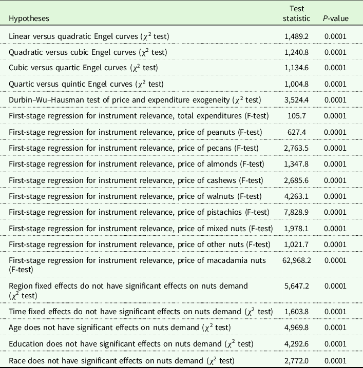
Note: Researcher(s)’ own analyses calculated (or derived) based in part on data from Nielsen Consumer LLC and marketing databases provided through the NielsenIQ Datasets at the Kilts Center for Marketing Data Center at The University of Chicago Booth School of Business.
The estimated DWH χ 2 statistic of 3,524.4 and its associated p-value of zero reject the null hypothesis of exogeneity and imply that total expenditure and prices are endogenous. Moreover, the results from the first-stage F-test decisively confirm that the expenditure and price instruments meet the relevance criterion (the p-value is equal to less than 0.0001). Finally, the p-value of the χ2 statistic (0.0001) implies that regional and time fixed effects significantly contribute to the explanatory power of the EASI model. A similar conclusion is reached for age, education, and race variables (p-value = 0.0001).
The parameter estimates from the expenditure and price equations are not reported for brevity (they are available upon request). However, the vast majority of the parameter estimates indeed are statistically significant at the 1% significance level, possessing the anticipated signs. Table 3 shows the parameter estimates, the corresponding standard errors, and the goodness-of-fit (R2) statistics from the EASI demand model.Footnote 2 The R2s, computed by squaring the correlation coefficient of actual and predicted values of the dependent variable, range from 0.0004 (macadamia nuts) to 0.0335 (other nuts). Most of the parameter estimates are statistically significant at the conventional significance levels. In particular, household income is negatively related to the budget shares of peanuts, walnuts, other nuts, and macadamia nuts, while positively affecting the budget shares of pecans, almonds, cashews, pistachios, and mixed nuts. An increase in the household size leads to an increase in the budget shares of peanuts, pecans, cashews, pistachios, and mixed nuts, and to a decrease in the budget shares of other nuts and macadamia nuts.
Table 3. Parameter estimates, standard errors, and goodness-of-fit statistics (R2) from the EASI demand model
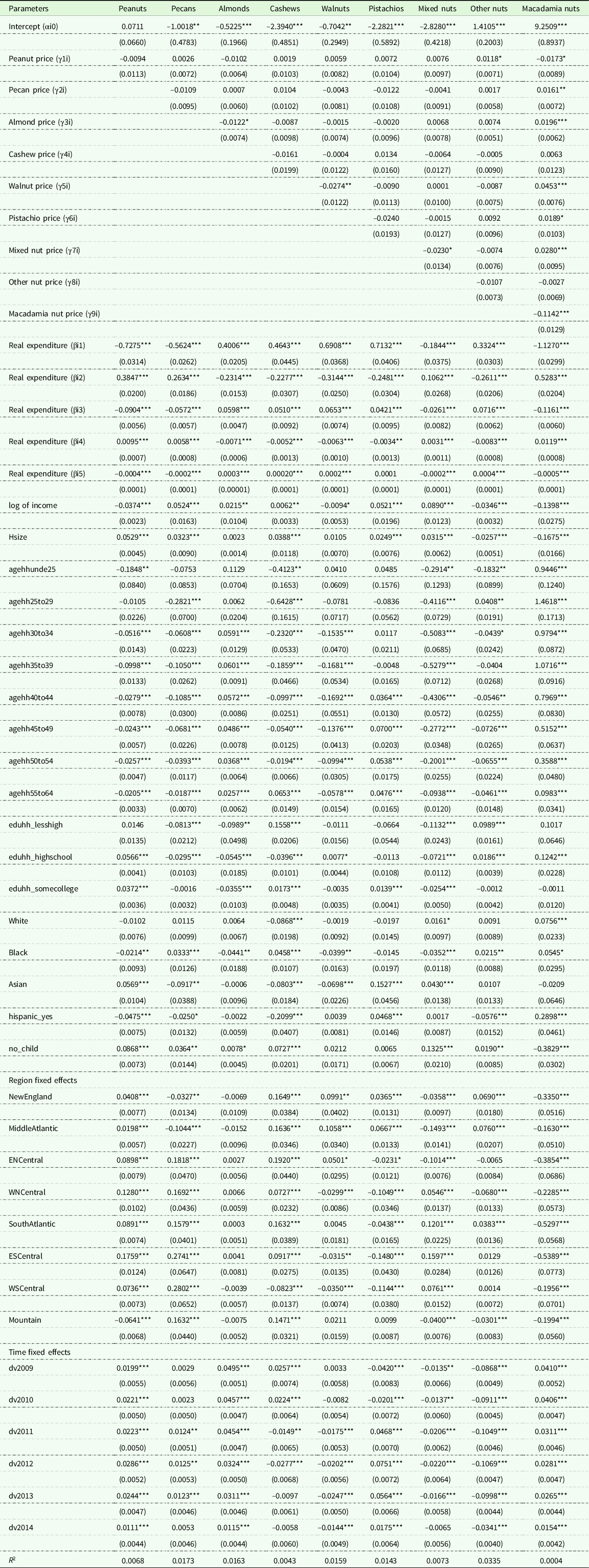
Note: Values in parentheses are the standard errors. Single, double, and triple asterisks (*,**,***) indicate statistical significance at the 10%, 5%, and 1% level, respectively.
Researcher(s)’ own analyses calculated (or derived) based in part on data from Nielsen Consumer LLC and marketing databases provided through the NielsenIQ Datasets at the Kilts Center for Marketing Data Center at The University of Chicago Booth School of Business.
Compared to households with heads aged above 64 years, households with heads aged under 25 years allocate higher shares of their nut expenditures to macadamia nuts and lower shares of their nut expenditures to peanuts, cashews, mixed nuts, and other nuts. Compared to households with heads aged above 64 years, households with heads aged between 25 and 29 years allocate higher shares of their nut expenditures to other nuts and macadamia nuts, and lower shares of their nut expenditures to pecans, cashews, and mixed nuts. Compared to households with heads aged above 64 years, households with heads aged between 30 and 34 years tend to allocate higher shares of their nut expenditures to almonds and macadamia nuts, and lower shares of their nut expenditures to peanuts, pecans, cashews, walnuts, mixed nuts, and other nuts. Compared to households with heads aged above 64 years, households with heads aged between 35 and 39 years tend to allocate higher shares of their nut expenditures to almonds and macadamia nuts, and lower shares of their nut expenditures to peanuts, pecans, cashews, walnuts, and mixed nuts. Compared to households with heads aged above 64 years, households with heads aged between 40 and 44 years, between 45 and 49 years, and between 50 and 54 years allocate higher shares of their nut expenditures to almonds, pistachios, and macadamia nuts, and lower shares of their nut expenditures to peanuts, pecans, cashews, walnuts, mixed nuts, and other nuts. Compared to households with heads aged above 64 years, households with heads aged between 55 and 64 years allocate higher shares of their nut expenditures to almonds, cashews, pistachios, and macadamia nuts, and lower shares of their nut expenditures to peanuts, pecans, walnuts, mixed nuts, and other nuts.
Relative to households with heads who have a college degree, households with heads who have less than high school education have higher budget shares for cashews and other nuts, but lower budget shares for pecans, almonds, and mixed nuts. Relative to households with heads who have a college degree, households with heads who have high school education have higher budget shares for peanuts, walnuts, other nuts, and macadamia nuts, but lower budget shares for pecans, almonds, cashews, and mixed nuts. Relative to households with heads who have a college degree, households with heads who have some college education have higher budget shares for peanuts, cashews, and pistachios, but lower budget shares for almonds and mixed nuts.
Households with White heads have higher budget shares for mixed nuts and macadamia nuts, but lower budget shares for cashews as opposed to households with heads of other races. Households with Black heads allocate more of their nut expenditures to pecans, cashews, other nuts, and macadamia nuts but allocate less of their nut expenditures to peanuts, almonds, walnuts, and mixed nuts, as opposed to households with heads of other races. Households with Asian heads have higher budget shares for peanuts, pistachios, and mixed nuts, but lower budget shares for pecans, cashews, and walnuts, as opposed to households with heads of other races.
Hispanic households allocate more of their nut expenditures to pistachios and macadamia nuts, and less of their nut expenditures to peanuts, pecans, cashews, and other nuts, as opposed to non-Hispanic households. Budget shares for peanuts, pecans, almonds, cashew, mixed nuts, and other nuts are higher for households with no children aged below 18 years, in contrast to households with at least one child aged below 18 years. But households with no children aged below 18 years have lower budget shares for macadamia nuts, in contrast to households with at least one child aged below 18 years.
Compared to households living in the Pacific region, households living in New England and Middle Atlantic regions allocate more of their nut expenditures to peanuts, cashews, walnuts, pistachios, and other nuts and allocate less of their nut expenditures to pecans, mixed nuts, and macadamia nuts. Compared to households living in the Pacific region, households living in the East North Central region allocate more of their nut expenditures to peanuts, pecans, cashews, and walnuts and allocate less of their nut expenditures to pistachios, mixed nuts, and macadamia nuts. Compared to households living in the Pacific region, households living in the West North Central region allocate more of their nut expenditures to peanuts, pecans, cashews, and mixed nuts and allocate less of their nut expenditures to walnuts, pistachios, other nuts, and macadamia nuts. Compared to households living in the Pacific region, households living in the South Atlantic region allocate more of their nut expenditures to peanuts, pecans, cashews, mixed nuts, and other nuts and allocate less of their nut expenditures to pistachios and macadamia nuts. Compared to households living in the Pacific region, households living in the East South Central region allocate more of their nut expenditures to peanuts, pecans, cashews, and mixed nuts and allocate less of their nut expenditures to walnuts, pistachios, and macadamia nuts. Compared to households living in the Pacific region, households living in the West South Central region allocate more of their nut expenditures to peanuts, pecans, and mixed nuts and allocate less of their nut expenditures to cashews, walnuts, pistachios, and macadamia nuts. Compared to households living in the Pacific region, households living in the Mountain region allocate more of their nut expenditures to pecans and cashews and allocate less of their nut expenditures to peanuts, mixed nuts, other nuts, and macadamia nuts.
Table 4 depicts uncompensated (Marshallian) own-price, cross-price, expenditure, and income elasticities of demand from the EASI model computed at the sample means. All the uncompensated own-price elasticities of demand are statistically significant, negative, as anticipated, and are greater than one in absolute value, implying that the demand for all nuts is elastic. This result may be attributed to the large number of available substitutes in the nut category. In particular, the magnitudes of own-price elasticities of demand for peanuts (–1.0149), pecans (–1.0368), almonds (–1.0464), cashews (–1.0512), walnuts (–1.0982), pistachios (–1.0820), mixed nuts (–1.0742), other nuts (–1.0567), and macadamia nuts (–2.3836) were different from those reported by Cheng, Capps, and Dharmasena (Reference Cheng, Capps and Dharmasena2021b). In the aforementioned study, the own-price elasticities for the same nut categories were as follows: peanuts (–1.5238), pecans (–1.8623), almonds (–2.0846), cashews (–2.0790), walnuts (–0.7385), macadamia nuts (–1.8942), pistachios (–0.3139), mixed nuts (–1.7782), and other nuts (–1.5492). Differences are attributed to functional form (QUAIDS versus EASI), time period 2004 to 2015 as opposed to 2009 to 2015, and level of aggregation (household versus market). Except for walnuts, macadamia nuts, and pistachios, the own-price elasticities of demand were larger in the Cheng, Capps, and Dharmasena study (Reference Cheng, Capps and Dharmasena2021b) compared to our study based on the EASI demand system.
Table 4. Uncompensated (Marshallian) price, expenditure, income elasticity estimates, and associated standard errors from the EASI demand model
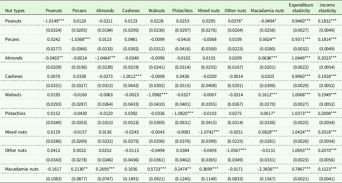
Note: Elasticities are calculated at the sample means. Values in the parentheses are the standard errors. Single, double, and triple asterisks (*,**,***) indicate statistical significance at the 10%, 5%, and 1% level, respectively. Researcher(s)’ own analyses calculated (or derived) based in part on data from Nielsen Consumer LLC and marketing databases provided through the NielsenIQ Datasets at the Kilts Center for Marketing Data Center at The University of Chicago Booth School of Business.
All expenditure elasticities are positive and statistically significant. Based on the expenditure elasticities, peanuts (0.9460), pecans (0.9371), cashews (0.9960), and macadamia nuts (0.7867) emerge as less responsive to changes in expenditure, whereas almonds (1.0449), walnuts (1.0068), pistachios (1.0373), mixed nuts (1.0424), and other nuts (1.0693) are more responsive. These findings are consistent with the results obtained by Lopez and Grigoryan (Reference Lopez and Grigoryan2018) and Asci and Devadoss (Reference Asci and Devadoss2021). As expected, all estimated income elasticities are positive and statistically significant. The values of income elasticity for peanuts (0.1832), pecans (0.1814), almonds (0.2023), cashews (0.1928), walnuts (0.1949), pistachios (0.2008), mixed nuts (0.2018), other nuts (0.2070), and macadamia nuts (0.1523) indicate that all the nut types are necessities in economic parlance. This finding was not completely in accord with the empirical results by Cheng, Capps, and Dharmasena (Reference Cheng, Capps and Dharmasena2021b). Although the respective nut categories were found to be necessities in their study, the magnitude of the income elasticities were roughly three to four times larger in the Cheng, Capps, and Dharmasena study (Reference Cheng, Capps and Dharmasena2021b).
Table 5 shows the estimated compensated (Hicksian) own-price elasticity of demand from the EASI model calculated at the sample mean values. Per the estimation results in Table 5, similar to the uncompensated own-price elasticities, all compensated own-price elasticities of demand are negative and statistically significant, ranging from –2.3813 (macadamia nuts) to –0.8028 (peanuts). As anticipated, the vast majority of compensated cross-price elasticities are statistically significant and positive, suggestive of net substitutability relationships among the nut types. Specifically, the strongest significant relationship is observed between macadamia nuts and walnuts (0.6573), while the weakest significant relationship is between mixed nuts and other nuts (0.0494). At the same time, a significant complementarity relationship is evident only between peanuts and macadamia nuts (–0.0467). The net substitutability relationship among nut types also was empirically established by Lopez and Grigoryan (Reference Lopez and Grigoryan2018). Cheng, Capps, and Dharmasena (Reference Cheng, Capps and Dharmasena2021b) not only found evidence of net substitutes among nut products but also found evidence of net complements as well. That said, substitution relationships were more common than complementary relationships.
Table 5. Compensated (Hicksian) price elasticity estimates and associated standard errors from the EASI demand model
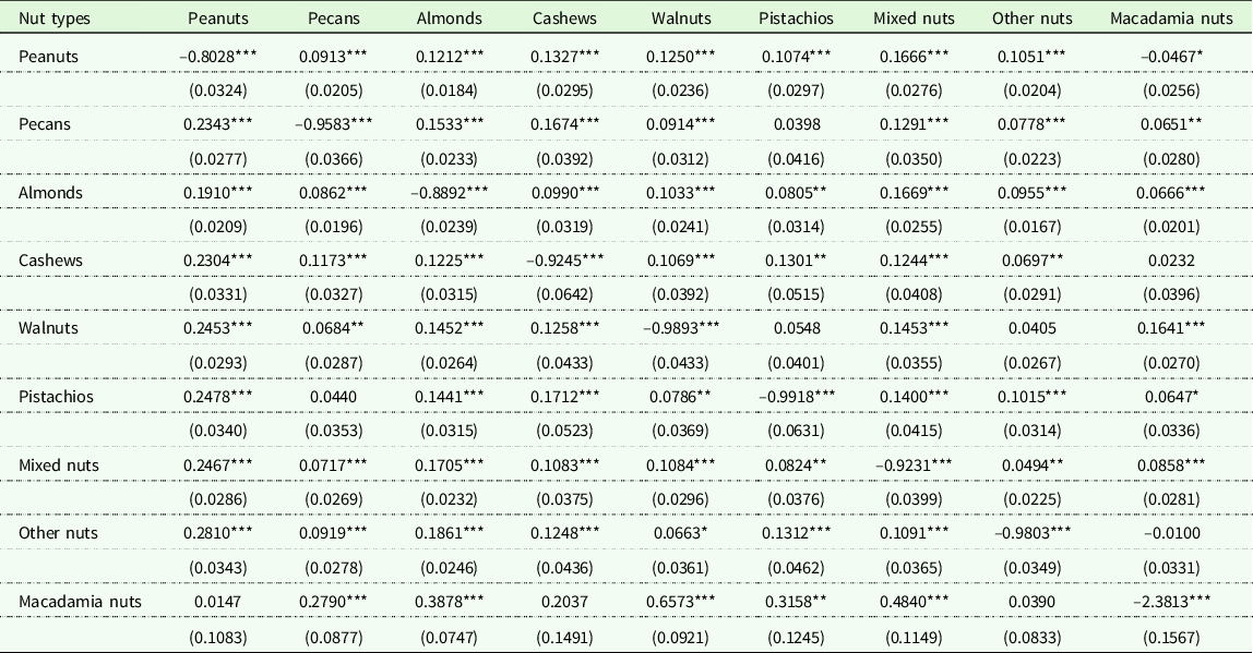
Note: Elasticities are calculated at the sample means. Values in the parentheses are the standard errors. Single, double, and triple asterisks (*,**,***) indicate statistical significance at the 10%, 5%, and 1% level, respectively. Researcher(s)’ own analyses calculated (or derived) based in part on data from Nielsen Consumer LLC and marketing databases provided through the NielsenIQ Datasets at the Kilts Center for Marketing Data Center at The University of Chicago Booth School of Business.
Finally, we simulate the effects of changing promotion expenditures on nut prices and quantities demanded. In general, promotion programs are designed to benefit producers and other interested parties in the supply chain in the form of expanded sales, heightened consumer awareness, and an overall increased demand. Not unlike other commodity organizations, promotion programs also have been implemented for different types of nuts. To foster the marketing and promotion of almonds, walnuts, pistachios, and pecans, various Federal Marketing Orders were put into place under the auspices of the Agricultural Marketing Service. In 1948, Federal Marketing Order 984 established the California Walnut Board. In 1950, Federal Marketing Order 981 established the Almond Board of California. In 2004, Federal Marketing Order 983 established the Administrative Committee for Pistachios. Most recently, in 2016, Federal Marketing Order 986 established the American Pecan Council. As such, the growth in the domestic demand for peanuts and tree nuts has been buoyed in part by their promotion as nutritious and healthy snacks by marketing boards and trade associations (Capps and Williams Reference Cheng, Capps and Dharmasena2021).
Based on this background information, a simulation exercise is conducted, where we use the information on the uncompensated own-price elasticities of demand from the present study ( $e_{ij}^U$
), the own-price elasticity of supply (
$e_{ij}^U$
), the own-price elasticity of supply ( $e_{ij}^S$
) from prior studies (for almonds and walnuts from Russo, Green and Howitt (Reference Russo, Green and Howitt2008), for peanuts from Beghin and Matthey (Reference Beghin and Matthey2003), and for the rest of the nuts from Okrent and Alston (Reference Okrent and Alston2012), since no other nut-specific own-price elasticity of supply information was available). Also, the base value of promotion expenditure elasticity for pecans of 0.0654 is taken from Capps and Williams (Reference Capps and Williams2021). This figure was calculated as the average of promotion expenditure elasticities for pecans from 2016 through 2020 (Capps and Williams Reference Cheng, Capps and Dharmasena2021). Lastly, Alston et al. (Reference Alston, Crespi, Kaiser and Sexton2007) estimated the promotion expenditure elasticity for almonds to be 0.13, and Kaiser (Reference Kaiser2018) estimated the promotion expenditure elasticity for walnuts to be 0.012, with both promotion expenditure elasticities being utilized in the simulation exercise. For the rest of the nut types that did not have an empirically estimated promotion expenditure elasticity, the base value of promotion expenditure elasticity for pecans is used.
$e_{ij}^S$
) from prior studies (for almonds and walnuts from Russo, Green and Howitt (Reference Russo, Green and Howitt2008), for peanuts from Beghin and Matthey (Reference Beghin and Matthey2003), and for the rest of the nuts from Okrent and Alston (Reference Okrent and Alston2012), since no other nut-specific own-price elasticity of supply information was available). Also, the base value of promotion expenditure elasticity for pecans of 0.0654 is taken from Capps and Williams (Reference Capps and Williams2021). This figure was calculated as the average of promotion expenditure elasticities for pecans from 2016 through 2020 (Capps and Williams Reference Cheng, Capps and Dharmasena2021). Lastly, Alston et al. (Reference Alston, Crespi, Kaiser and Sexton2007) estimated the promotion expenditure elasticity for almonds to be 0.13, and Kaiser (Reference Kaiser2018) estimated the promotion expenditure elasticity for walnuts to be 0.012, with both promotion expenditure elasticities being utilized in the simulation exercise. For the rest of the nut types that did not have an empirically estimated promotion expenditure elasticity, the base value of promotion expenditure elasticity for pecans is used.
Following Lusk and Tonsor (Reference Lusk and Tonsor2021), we plug these values into the following expressions to compute the percentage change in price: %ΔP = (S
d
− S
s
)/( $\;e_{ij}^S$
-
$\;e_{ij}^S$
- $e_{ij}^U$
), and the percentage change in quantity demanded: %ΔQ = E
d
×(%ΔP) + S
d
, where S
d
represents the percentage change in quantity demanded due to a change in the value of promotion expenditure elasticity, S
s
represents the percentage change in quantity supplied due to a change in the value of any right-hand side supply shifter other than own price (in this case, we assume that S
s
is zero since promotion expenditure is a demand shifter). Both %ΔP and %ΔQ are computed for the base value of promotion expenditure elasticity and its alternative values (base value: +1%, +5%, and +10%). We recognize that the alternative values for promotion elasticities indeed are arbitrary. That said, the simulation process remains the same no matter the magnitude of the promotion elasticity.
$e_{ij}^U$
), and the percentage change in quantity demanded: %ΔQ = E
d
×(%ΔP) + S
d
, where S
d
represents the percentage change in quantity demanded due to a change in the value of promotion expenditure elasticity, S
s
represents the percentage change in quantity supplied due to a change in the value of any right-hand side supply shifter other than own price (in this case, we assume that S
s
is zero since promotion expenditure is a demand shifter). Both %ΔP and %ΔQ are computed for the base value of promotion expenditure elasticity and its alternative values (base value: +1%, +5%, and +10%). We recognize that the alternative values for promotion elasticities indeed are arbitrary. That said, the simulation process remains the same no matter the magnitude of the promotion elasticity.
Table 6 shows the own-price demand, own-price supply, and alternative promotion expenditure elasticities, and the corresponding simulated percentage changes in prices and quantities demanded for all nut types. As the figures in Table 6 demonstrate, for 1% increase in promotion expenditure elasticity from its base case, prices for all nuts increase with the lowest percentage change increase of 0.0171 recorded for walnuts and the highest percentage change increase of 0.0816 recorded for almonds. Additionally, a 5% increase in promotion expenditure elasticity from its base case leads to the lowest percentage change of 0.0409 for macadamia nut price and to the highest percentage change of 0.1049 for almond price. And, for a 10% increase in promotion expenditure elasticity from its base case, the percentage change in price ranges from the lowest of 0.0586 (macadamia nut) to the highest of 0.1340 (almonds).
Table 6. Effects of changing promotion expenditure elasticities on nut prices and quantities
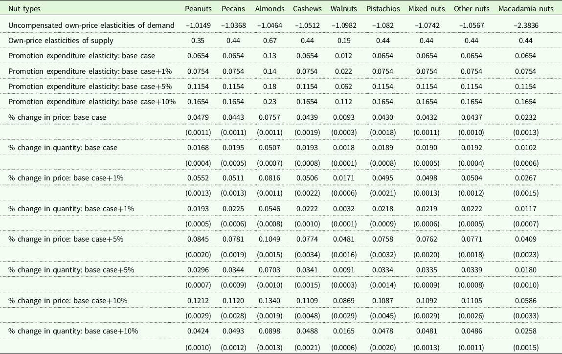
Note: Uncompensated own-price elasticities of demand are computed in the present study. The estimate of the own-price elasticity of supply of peanuts is borrowed from Beghin and Matthey (Reference Beghin and Matthey2003), the estimates of the own-price elasticity of supply of almonds and walnuts are borrowed from Russo, Green, and Howitt (Reference Russo, Green and Howitt2008), and the estimate of the own-price elasticity of supply of the rest of the nut types is borrowed from Okrent and Alston (Reference Okrent and Alston2012). The average promotion expenditure elasticity of pecans of 0.0654 is taken from Capps and Williams (Reference Capps and Williams2021), the promotion expenditure elasticity of 0.13 for almonds is taken from Alston et al. (Reference Alston, Crespi, Kaiser and Sexton2007), and the promotion expenditure elasticity of 0.012 for walnuts is taken from Kaiser (Reference Kaiser2018). Values in the parentheses are the standard errors around the simulated price and quantity calculated using a stochastic simulation procedure in SIMETAR statistical software (Richardson, Schumann, and Feldman Reference Richardson, Schumann and Feldman2008).
A 1% increase in promotion expenditure elasticity from its base case leads to an increase in percentage change in quantity demanded of all nut types varying from the lowest change of 0.0032 (walnuts) to the highest change of 0.0546 (almonds). Also, a 5% increase in promotion expenditure elasticity from its base case results in the lowest percentage change increase of 0.0091 for walnuts and the highest percentage change increase of 0.0703 for almonds. Finally, for a 10% increase in promotion expenditure elasticity from its base case, the percentage change in quantity demanded ranges from the lowest of 0.0165 (walnuts) to the highest of 0.0898 (almonds).
Conclusions and recommendations for future research
This study analyzes the interrelationships of household demand for peanuts and various tree nuts. To that end, the fixed-effect LA-EASI model is estimated taking into account unobserved household preference heterogeneity, flexible Engel curves, total expenditure and price endogeneity, data censoring as well as region- and time-specific unobservable effects. The household-level panel data used in this study are derived from the Nielsen Homescan panels from calendar years 2009 through 2015. The data pertain to prices and quantities of peanuts, pecans, almonds, cashews, walnuts, pistachios, mixed nuts, macadamia nuts, and other nuts as well as sociodemographic characteristics of participant households.
As evidenced by the empirical results, the quintic (fifth) degree EASI model was favored over other degrees in real expenditures, an important finding that shows that linear and quadratic real expenditures, oftentimes used in empirical work, may not be the “best” ones to apply. The empirical results demonstrate that the demands for all nuts are elastic. Given the sensitivity of households to changes in prices, nut producers and purveyors should center attention on lowering prices in order to maximize their short-run total revenue. Per the compensated cross-price elasticities of demand, nuts are substitutes for each other. This information is useful to stakeholders in the industry in terms of their input procurement and inventory management decisions in response to changes in prices of competing nut types. According to the income elasticity estimates, all the nuts emerge as necessities. As such, households are not particularly sensitive to changes in household income.
A set of household demographic characteristics are statistically significant drivers of the demand for nuts. This information can be used by nut producers and nut purveyors in terms of designing marketing strategies aimed at expanding their customer base. Finally, this study uses demand and supply elasticities to simulate the effects of changes in the magnitude of a selected promotion expenditure elasticity on the prices and quantities demanded of nuts. The computed changes in prices and quantities of nuts resulting from corresponding changes in promotion expenditure elasticities can be used by policy makers, the Almond Board of California, the Walnut Marketing Board, the American Pecan Council, and the California Pistachio Research Board in designing promotion programs as well as price and production control programs.
A few recommendations for future research are worth noting. First, conditional upon the availability of such information, future research would benefit from using cost data to serve as instruments for prices. Second, if available, it would be appealing for future research to also incorporate information on relevant away-from-home consumption, since the Nielsen Homescan data used in this study provide information only for at-home consumption. Third, it would be worthwhile for future research to allow for possible seasonality in the consumption of nuts by using monthly or quarterly data. Despite these recommendations, the present research makes solid contributions to the extant literature.
Supplementary material
To view supplementary material for this article, please visit https://doi.org/10.1017/age.2022.11
Acknowledgments
Researcher(s)’ own analyses calculated (or derived) based in part on: (i) retail measurement/consumer data from Nielsen Consumer LLC (“NielsenIQ”); (ii) media data from The Nielsen Company (US), LLC (“Nielsen”); and (iii) marketing databases provided through the respective NielsenIQ and the Nielsen Datasets at the Kilts Center for Marketing Data Center at The University of Chicago Booth School of Business. The conclusions drawn from the Nielsen data are those of the researcher(s) and do not reflect the views of NielsenIQ or Nielsen. Neither NielsenIQ nor Nielsen is responsible for, had any role in, or was involved in analyzing and preparing the results reported herein.
Author contributions
Study conception and design: Oral Capps, Jr., Guo “Chris” Cheng, Senarath Dharmasena; data collection: Guo “Chris” Cheng, Senarath Dharmasena; analysis and interpretation of results: Rafael Bakhtavoryan, Oral Capps, Jr.; draft manuscript preparation: Rafael Bakhtavoryan, Oral Capps, Jr., Guo “Chris” Cheng, Senarath Dharmasena. All authors reviewed the results and approved the final version of the manuscript.
Funding statement
This research received no specific grant from any funding agency, commercial, or not-for-profit sectors.
Competing interests
The author(s) declare none.
Ethical standards
This article does not contain any studies involving human participants performed by any of the authors.


 Open access