

In the United States, a farmers market (FM) is a common area where farmers gather on a recurring basis to sell a range of products including fresh fruits and vegetables, and other farm products, directly to consumers (Martinez et al. Reference Martinez, Hand, Da Pra, Pollack, Ralston, Smith, Vogel, Clark, Lohr, Low and Newman2010). The USDA Agricultural Marketing Service reports that from 1994 to 2015 the number of FMs in the United States has increased from 1,755 units to 8,476. However, growth rates have slowed in recent years, from 1.5 percent to 2.5 percent.
Several benefits have been associated with the presence of short food supply chains, of which FMs are an example. From the participant farmers’ (i.e., vendors’) standpoint, direct channels allow them to avoid intermediaries and retailers and, as a result, to realize a higher share of the channel's profits (La Trobe Reference La Trobe2001). Besides internalizing higher margins, participating farmers can have direct access to consumers with higher willingness to pay for locally produced foods (Gilg and Battershill Reference Gilg and Battershill1998). FMs can also give vendors greater ability to launch and test new products (Brown Reference Brown2002, Brown and Miller Reference Brown and Miller2008).
FMs are found to provide societal benefits including positive community-wide impacts such as human capital building (Brown Reference Brown2002, Brown and Miller Reference Brown and Miller2008), facilitation of social interaction, promotion and development of trust and social capital (Hunt Reference Hunt2007), and a stronger sense of connection between consumers and the local community (Gale Reference Gale1997). For consumers, FMs may increase customer satisfaction due to freshness and quality of products (Govindasamy et al. Reference Govindasamy, Italia, Zurbriggen and Hossain2002), and may lead to increased consumption of fruit and vegetables and other “wholesome” foods. A few authors also suggest that FMs can contribute to improved diets and a reduction in childhood obesity (Frieden, Dietz, and Collins Reference Frieden, Dietz and Collins2010). To this point, Berning (Reference Berning2012) finds higher densities of FMs and community supported agricultureFootnote 1 to be inversely related to individual weight outcomes in the United States, while Bimbo et al. (Reference Bimbo, Bonanno, Nardone and Viscecchia2015) find a negative correlation between FMs’ presence and adults’ BMI in Italy. More generally, Salois (Reference Salois2012) finds the presence of short food supply chains to have a negative association with obesity rates and diabetes’ prevalence.
The rapid growth of FMs in the United States has been promoted by policymakers who aim to expand the sales of locally produced food and agricultural commodities (see Martinez et al. Reference Martinez, Hand, Da Pra, Pollack, Ralston, Smith, Vogel, Clark, Lohr, Low and Newman2010, for a summary of federal, state and local policies supporting local food production) while also attempting to improve access to food for underserved individuals. The 2014 Farm Bill supports directly the development of more FMs via the direct marketing grants program of the Farmers Market Promotion Program (FMPP). Indirectly, the Local Food Promotion Program (LFPP) aims to strengthen the structure of local food supply chains. Furthermore, many FMs have adopted strategies targeting low-income consumers by accepting Electronic Benefit Transfer (EBT) from the Supplemental Nutrition Assistance Program (SNAP). A Congressional Research Service report indicates that 2,445 FMs and farmers were authorized to accept SNAP in 2011, and the redeemed benefits totaled $11.7 million (Johnson, Alison and Cowan, Reference Johnson, Alison and Cowan2013). These figures represent a 51 percent increase in authorizations and more than a 55 percent increase in redeemed benefits compared to 2010. As of July 2014, about two thirds of the states authorized farmers to accept cash value vouchers from the Women, Infants and Children (WIC) program through the Farmers Market Nutrition Program (FMNP).Footnote 2
Given the increasing interest of policymakers and local planners in promoting FMs, and the potential benefits associated with them, it is both relevant and timely to evaluate the economic factors facilitating and supporting their development. The geographic dispersion of FMs shows higher numbers along the coasts, predominantly in proximity to highly populated areas in California, in the northeast, and surrounding the Great Lakes (Martinez et al. Reference Martinez, Hand, Da Pra, Pollack, Ralston, Smith, Vogel, Clark, Lohr, Low and Newman2010). This can be attributable to the fact that, to be successful, FMs must attract both sufficient numbers of vendors and consumers to a single location. Thus, areas where more FMs exist can be found in easy to reach, populated areas, with a relatively high level of farming activities. At the same time, vendors face higher competition in areas with higher demand, which can be costly (Lohr et al. Reference Lohr, Diamond, Dicken and David2011). While less populous areas may not be current hot spots of growth for FMs, they could represent lower-cost options for producers if sufficient demand exists to support their economic viability.
Anecdotal evidence suggests that the continued expansion of FMs over the last few years may mask high failure rates.Footnote 3 Several factors are found to be affecting the likelihood of FMs market failures (Stephenson, Lev, and Brewer Reference Stephenson, Lev and Brewer2008). While areas most suited for supporting one or more FMs may already be saturated, areas less suited for supporting FMs, either because of limited demand or infrastructure, may be those that remain unserved, making policy efforts to promote FM expansion harder to be implemented.Footnote 4 While academic research has attempted to characterize FM shoppers and their motivations for patronizing these outlets (e.g., Wolf, Spittler, and Ahern Reference Wolf, Spittler and Ahern2005, Zepeda Reference Zepeda2009, Pascucci et al. Reference Pascucci, Cicatiello, Franco, Pancino and Marino2011, Gumirakiza, Curtis, and Bosworth Reference Gumirakiza, Curtis and Bosworth2014) and to assess the factors that affect the performance of their vendors (e.g., Schmidt and Gómez Reference Schmidt and Gómez2011, Varner and Otto Reference Varner and Otto2008), with the exception of Lohr et al. (Reference Lohr, Diamond, Dicken and David2011) and Singleton, Sen, and Affuso (Reference Singleton, Sen and Affuso2015), little is known of the market forces driving FM formation.
In this article we assess the demand- and supply-side conditions that facilitate FM creation. To achieve this objective we create a theoretical model of a farmer's decision to engage in an FM and determine an expression for the equilibrium number of farmers willing to participate. Based on this result, we parameterize different specifications of a reduced-form empirical model to estimate how specific market factors affect the probability of observing one or two or more FMs in a given area.
We choose the New England states as a case study for two reasons. First, while the northeast is one of the areas showing the highest prevalence of FMs (see Martinez et al. Reference Martinez, Hand, Da Pra, Pollack, Ralston, Smith, Vogel, Clark, Lohr, Low and Newman2010 pg. 8), in the year prior to our sample year (2012) New England presented one of the largest areas of growth in FMs, well above the national rates (14.4 percent, second only to the mid-Atlantic, 15.8 percent) (USDA, Reference Zepeda2012). Second, as illustrated in more detail in the data section, while there is a relatively high variation in the number of FMs across zip codes in New England, the size of each zip code (in terms of square miles) is less heterogeneous in these states compared to other parts of the nation, which can reduce unobserved heterogeneity bias.
Our results indicate that market size, presence of children in the household, a more educated and younger population, and a higher percentage of individuals in SNAP, are more likely to foster the location of FMs, as well as a higher pool of potential participant vendors. Also, the opportunity cost of selling area, used as a proxy for establishments’ costs, is associated with a lower probability of observing more FMs, and while the presence of alternative distribution channels (that is, fruit and vegetable wholesalers) is inversely related to the likelihood of observing FMs, grocery stores seem to act as complements.
A Model for Farmers Market Formation and Location
Assume that, in a given geographic market, there are M farmers who decide through which marketing channel to sell their product, the FM channel (a), the traditional retail channel (b) or both. The total market size for a given geographic area is S. Consumers can shop in both channels: a fraction λ prefers the FM marketing channel (S a = λS), while the rest prefer traditional channels or S b = (1 − λ)S. Therefore, S = S a + S b =λS+ (1 − λ)S.
Consider the ith farmer (i = 1 to M), whose potential sales from the FM channel (S
ia
) and traditional channel (S
ib
) are determined by the number of participants in each channel, or $S_{ia} = \displaystyle{{S_a} \over {m_a}} = \displaystyle{{\lambda S{\rm \; }} \over {m_a}}$
and
$S_{ia} = \displaystyle{{S_a} \over {m_a}} = \displaystyle{{\lambda S{\rm \; }} \over {m_a}}$
and $S_{ib} = \displaystyle{{S_b} \over {m_b}} = \displaystyle{{\left({1 - \; \lambda} \right)S} \over {m_b}}$
, where m
a
and m
b
are homogenous farms participating in the FM channel and in the traditional channel, respectively. Each channel price (P) is determined by the market and the average variable cost (AVC) for producing and selling products in each channel is assumed constant. The per-unit margin for products sold through each channel j is θ
j
≡ (P
j
− AVC
j
) where j = [a, b].
$S_{ib} = \displaystyle{{S_b} \over {m_b}} = \displaystyle{{\left({1 - \; \lambda} \right)S} \over {m_b}}$
, where m
a
and m
b
are homogenous farms participating in the FM channel and in the traditional channel, respectively. Each channel price (P) is determined by the market and the average variable cost (AVC) for producing and selling products in each channel is assumed constant. The per-unit margin for products sold through each channel j is θ
j
≡ (P
j
− AVC
j
) where j = [a, b].
To participate in the FM channel, each farmer pays a fee (F) that is determined by establishment costs (E), assumed to be evenly distributed across participants or F = E/m a . The establishment costs include selling area rental expenses, and utility costs, advertising, and marketing for the FM and any other management and maintenance costs required to create, maintain, and organize the FM.Footnote 5
In the simplest case (Scenario 1), farmers participate in only one of the channels. This implies that M = m
a
+ m
b
and that $S_{ia} = \displaystyle{{\lambda S} \over {m_a}}$
and
$S_{ia} = \displaystyle{{\lambda S} \over {m_a}}$
and $S_{ib} = \displaystyle{{\left({1 - \; \lambda} \right)S} \over {M - m_a}}$
. Similar to Sexton's (1986) work on cooperatives, participating in an FM is desirable for a farmer if:
$S_{ib} = \displaystyle{{\left({1 - \; \lambda} \right)S} \over {M - m_a}}$
. Similar to Sexton's (1986) work on cooperatives, participating in an FM is desirable for a farmer if:
 $$\psi _i = \pi _{ia} - \pi _{ib} = \theta_a \displaystyle{{\lambda S} \over {m_a}} - \theta_b \displaystyle{ {\lpar {1 - \; \lambda} \rpar S} \over {M - m_a}}\; - F\; \ge 0$$
When equation (1) is an equality, a farmer will be indifferent to participating in an FM or in the traditional channels. Manipulating this expression for the indifferent farmer, one can obtain the limiting number of farms participating in the FM channel:
 $$m_a^{\ast} = M\displaystyle{{\theta _a\lambda S - E} \over {\theta _b \lpar {1 - \lambda} \rpar S + \theta _a\lambda S - E}}\; \lpar \rm Scenario \;1\rpar$$
If equation (2) is continuous, it is easy to verify that participation decreases with establishment costs, although at declining rates $\bigg(\displaystyle{{\partial m_a^ \ast} \over {\partial E}} \lt 0$
,
$\bigg(\displaystyle{{\partial m_a^ \ast} \over {\partial E}} \lt 0$
, $\displaystyle{{\partial ^2m_a^*} \over {\partial E^2}} \gt 0\bigg)$
. Participation also decreases with the margin of the traditional channel at a decreasing rate
$\displaystyle{{\partial ^2m_a^*} \over {\partial E^2}} \gt 0\bigg)$
. Participation also decreases with the margin of the traditional channel at a decreasing rate $\bigg(\displaystyle{{\partial m_a^*} \over {\partial \theta _b}} \lt 0$
,
$\bigg(\displaystyle{{\partial m_a^*} \over {\partial \theta _b}} \lt 0$
, $\displaystyle{{\partial ^2m_a^*} \over {\partial \theta _b^2}} \gt 0\bigg)$
and increases at a decreasing rate with the margin for the FM channel
$\displaystyle{{\partial ^2m_a^*} \over {\partial \theta _b^2}} \gt 0\bigg)$
and increases at a decreasing rate with the margin for the FM channel $\bigg(\displaystyle{{\partial m_a^*} \over {\partial \theta _a}} \gt 0$
,
$\bigg(\displaystyle{{\partial m_a^*} \over {\partial \theta _a}} \gt 0$
, $\displaystyle{{\partial ^2m_a^*} \over {\partial \theta _a^2}} \lt 0\bigg)$
. Participation increases at a decreasing rate with the share of consumers preferring the short channel
$\displaystyle{{\partial ^2m_a^*} \over {\partial \theta _a^2}} \lt 0\bigg)$
. Participation increases at a decreasing rate with the share of consumers preferring the short channel $\bigg( \displaystyle{{\partial m_a^*} \over {\partial \lambda}} \gt 0$
,
$\bigg( \displaystyle{{\partial m_a^*} \over {\partial \lambda}} \gt 0$
, $\displaystyle{{\partial ^2m_a^*} \over {\partial \lambda ^2}} \lt 0\bigg)$
and increases linearly with the total number of farmers
$\displaystyle{{\partial ^2m_a^*} \over {\partial \lambda ^2}} \lt 0\bigg)$
and increases linearly with the total number of farmers $\bigg(\displaystyle{{\partial m_a^*} \over {\partial M}} \; \gt 0$
,
$\bigg(\displaystyle{{\partial m_a^*} \over {\partial M}} \; \gt 0$
, $\displaystyle{{\partial ^2m_a^*} \over {\partial M^2}} = 0\bigg)$
. Finally, participation increases at a decreasing rate with the total market size
$\displaystyle{{\partial ^2m_a^*} \over {\partial M^2}} = 0\bigg)$
. Finally, participation increases at a decreasing rate with the total market size $\bigg(\displaystyle{{\partial m_a^*} \over {\partial S}} \gt 0$
,
$\bigg(\displaystyle{{\partial m_a^*} \over {\partial S}} \gt 0$
, $\displaystyle{{\partial ^2m_a^*} \over {\partial S^2}} \lt 0\bigg)$
.
$\displaystyle{{\partial ^2m_a^*} \over {\partial S^2}} \lt 0\bigg)$
.
Alternatively, farmers have the ability to participate in both channels at once (Scenario 2). Farmers may do this for one of two reasons. First, in joining both channels, farmers can cater to different consumer types and spread production risk; these farmers may produce higher-quality products and will likely benefit the most from the FM channel.Footnote 6 Second, farmers selling primarily in traditional channels may treat the FM channel as an outlet for their excess supply, as they may see FMs as seasonal and less consistent than traditional channels. In both cases, farmers’ sales to each channel are determined by participation: in this case the decision to enter the FM channel only requires that variable profits exceed participation costs, or θ a λS ≥ E (in this second scenario, m a represents the number of farmers participating in the FM channel plus those participating in both channels). That is, a farmer will be more likely to participate in the FM channel if per-unit margin or consumer demand for FMs increases, or if the establishment costs decrease.
Let us consider now the creation of an FM. For the equilibrium number of FMs (N) in a given area to be strictly positive, enough farmers must be willing to participate. Thus, for an FM to exist, at least one farmer must find joining the FM channel profitable. In Scenario 1, participating in an FM requires the establishment fee to be bounded as $0 \lt E \lt \theta _a\lambda S - \displaystyle{{\left({1 - \lambda} \right)S\theta _b} \over {M - 1}}$
(because E is non-negative) while in Scenario 2 the condition to be satisfied is 0 <E <θ
a
λS. Thus, for the same levels of θ
a
, λ and S, joining an FM can still be profitable at higher participation fees in markets where farmers can join both channels (Scenario 2), than in those where participation in one channel is exclusive (Scenario 1). If program participation fees are reduced (that is, as E → 0), the maximum number of participating farmers is bounded by
$0 \lt E \lt \theta _a\lambda S - \displaystyle{{\left({1 - \lambda} \right)S\theta _b} \over {M - 1}}$
(because E is non-negative) while in Scenario 2 the condition to be satisfied is 0 <E <θ
a
λS. Thus, for the same levels of θ
a
, λ and S, joining an FM can still be profitable at higher participation fees in markets where farmers can join both channels (Scenario 2), than in those where participation in one channel is exclusive (Scenario 1). If program participation fees are reduced (that is, as E → 0), the maximum number of participating farmers is bounded by $m_a \in \left({1\comma \; M\displaystyle{{\theta _a\lambda S} \over {\theta _a\lambda S + \left({1 - \lambda} \right)S\theta _b}}} \right)$
in Scenario 1 and by M in Scenario 2. Thus, factors supporting the adoption of two channels (presence of alternative distribution systems, etc.) may create conditions more conducive to FM creation. These two results imply that it is more likely to observe a higher participation in Scenario 2 than in Scenario 1, or in other words, factors facilitating the adoption of two channels can foster higher N.
$m_a \in \left({1\comma \; M\displaystyle{{\theta _a\lambda S} \over {\theta _a\lambda S + \left({1 - \lambda} \right)S\theta _b}}} \right)$
in Scenario 1 and by M in Scenario 2. Thus, factors supporting the adoption of two channels (presence of alternative distribution systems, etc.) may create conditions more conducive to FM creation. These two results imply that it is more likely to observe a higher participation in Scenario 2 than in Scenario 1, or in other words, factors facilitating the adoption of two channels can foster higher N.
We assume that, once a minimum participation threshold is reached, there is a positive relationship between the number of farmers / vendors participating in the FM channel $m_a^* $
and the number of FMs N. Let us consider now N*, a realization of N. Define
$m_a^* $
and the number of FMs N. Let us consider now N*, a realization of N. Define $\bar m_{a\left({N^ \ast} \right)}$
as the minimum number of participating farmers necessary for the probability of observing at least N* FMs to be non-zero. For any
$\bar m_{a\left({N^ \ast} \right)}$
as the minimum number of participating farmers necessary for the probability of observing at least N* FMs to be non-zero. For any $m_a^ \ast $
strictly greater than
$m_a^ \ast $
strictly greater than $\bar m_{a\left({N^ \ast} \right)}$
one has:
$\bar m_{a\left({N^ \ast} \right)}$
one has:
 $$Pr\lsqb {N^{\ast} \gt 0\left \vert {m_a^{\ast} \lpar {\lambda, S,\theta _a,\theta _b,E,M} \rpar} \right\gt {\bar m}_{a\lpar {N^{\ast}} \rpar}} \rsqb \gt 0$$
Equation (3) indicates that even if there are some farmers wanting to join an FM, there need to be enough of them to support N* FMs. Generalizing, the number of FMs will be limited by the number of participating farmers such that:
 $$Pr \lsqb {N^{\ast} + 1 \vert {{\bar m}_{a\lpar{N^{\ast} + 1} \rpar}} \gt m_a^{\ast} \lpar. \rpar \ge {\bar m}_{a\lpar{N^{\ast}} \rpar}} \rsqb = 0 \comma$$
where $\bar m_{a \left({N^* + 1} \right)}$
is the minimum number of FMs required to establish N* + 1 FMs. In other words, if there are fewer than
$\bar m_{a \left({N^* + 1} \right)}$
is the minimum number of FMs required to establish N* + 1 FMs. In other words, if there are fewer than $\bar m_{a\left({N^* + 1} \right)}$
participant farmers it is not possible for N* + 1 farmers markets to formFootnote
7
. For any non-zero values of
$\bar m_{a\left({N^* + 1} \right)}$
participant farmers it is not possible for N* + 1 farmers markets to formFootnote
7
. For any non-zero values of $m_a^* \left(. \right)$
satisfying conditions (3) and (4), there will be an equilibrium number of FMs equal to N*. Intuitively, as a farmer-participation threshold is crossed, the probability that an additional FM is formed will increase. As participation grows, new thresholds are reached, and the probability of observing additional FMs increases.
$m_a^* \left(. \right)$
satisfying conditions (3) and (4), there will be an equilibrium number of FMs equal to N*. Intuitively, as a farmer-participation threshold is crossed, the probability that an additional FM is formed will increase. As participation grows, new thresholds are reached, and the probability of observing additional FMs increases.
The number of FM participants, as well as participation thresholds, are not observed, whereas the number of FMs and market characteristics influencing participation are. Thus, we treat participants’ numbers as a latent variable and recover the effect of different market characteristics by estimating the probability of observing a given number of FMs N*. To that end, we parameterize an expression for N* as a function of the factors affecting FM participation and estimate the link between the number of observed FMs and market characteristics determining participation. The probability of observing an area with at least N = N* FMs is
 $$Pr \lpar {N^{\ast} \gt N} \rpar = 1 - {\rm \Phi} \lpar {m_{a\lpar {N^{\ast}} \rpar}} \rpar$$
where Φ(.) is the standard normal cumulative density function and $m_{a\left({N^*} \right)} = m_a^* \left({\lambda\comma \; S\comma \; \theta _a\comma \; \theta _b\comma \; E\comma \; \; M} \right)+ \varepsilon $
represents the number of participating farmers satisfying the condition
$m_{a\left({N^*} \right)} = m_a^* \left({\lambda\comma \; S\comma \; \theta _a\comma \; \theta _b\comma \; E\comma \; \; M} \right)+ \varepsilon $
represents the number of participating farmers satisfying the condition $m_a^* \gt \bar m_{a\left({N^*} \right)}$
, while the probability of observing an area with exactly N* FMs is
$m_a^* \gt \bar m_{a\left({N^*} \right)}$
, while the probability of observing an area with exactly N* FMs is
 $$Pr \lpar {N^{\ast} \le \; N \lt N^{\ast} + 1} \rpar = {\rm \Phi} \lpar {m_{a\lpar {N^{\ast} + 1} \rpar}} \rpar - {\rm \Phi} \lpar {m_{a\lpar {N^{\ast}} \rpar}} \rpar.$$
For simplicity, we assume $m_a^* \left({\lambda\comma \; S\comma \; \theta _a\comma \; \theta _b\comma \; E\comma \; \; M} \right)= {\bi {X}^{\prime}\beta}$
, where
X
is a vector of covariates including elements that characterize the different factors affecting market participation, and
β
is a conformable vector of coefficients capturing the relationship between the different covariates and market participation. Given the assumptions illustrated above, estimates of the vector
β
are obtained using an ordered probit estimator.Footnote
8
$m_a^* \left({\lambda\comma \; S\comma \; \theta _a\comma \; \theta _b\comma \; E\comma \; \; M} \right)= {\bi {X}^{\prime}\beta}$
, where
X
is a vector of covariates including elements that characterize the different factors affecting market participation, and
β
is a conformable vector of coefficients capturing the relationship between the different covariates and market participation. Given the assumptions illustrated above, estimates of the vector
β
are obtained using an ordered probit estimator.Footnote
8
Data
We estimate the parameters of our model using a zip-code-level database encompassing the six New England states, assembled from different sources. Our data were collected in the spring of 2013 and represent a single cross-section. We acquired data on FMs’ zip code location from LocalHarvest, Inc. (localharvest.org), which provides a nationwide registry of FMs free of charge. In addition, LocalHarvest indicates the last time an FM's information was updated. While a large share of FMs update their LocalHarvest site regularly, for those that have not updated their site in the last two years, we determined whether the FM was still in operation using State-level Department of Agriculture listings of FMs and internet searches.Footnote 9 The initial data set is comprised of 1,833 zip codes. In New England, seventy seven percent of the zip codes do not have an FM, nineteen percent have at least one, and the remaining four percent has two or more FMs (Table 1).
Table 1. Frequency of FMs Within Zip Codes

We use total population in each zip code from the 2011 American Community Survey to characterize market size (S). Figure 1 shows the geographic distribution of FMs location (left panel) and population (right panel) in New England's zip codes. This map shows that FMs seem mostly located along the coasts and in proximity to large urbanized areas, and that areas with higher populations are more attractive as the location of one or more FMs.
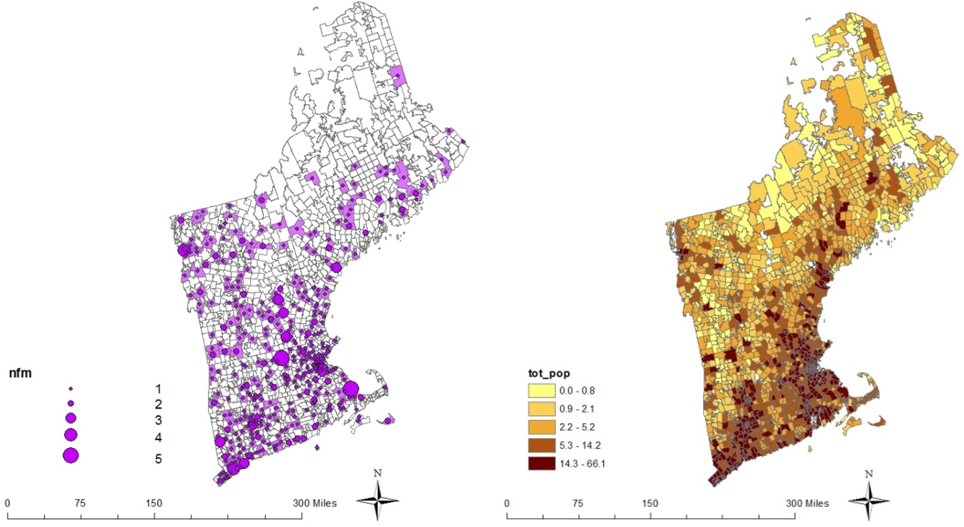
Figure 1. Zip-Code-Level Location of FMs (Left Panel) and Total Population (tot_pop) in New England
Variables capturing factors affecting consumer preferences for FMs (i.e. λ) also come from the American Community Survey. First, we control for the share of household with children, median age in the zip code, as well as the average household size in the zip code, as the size of the household affects the likelihood of shopping at FMs (Gumirakiza, Curtis, and Bosworth Reference Gumirakiza, Curtis and Bosworth2014). As ethnicity seems to be correlated with FMs’ location (Singleton, Sen, and Affuso Reference Singleton, Sen and Affuso2015), we control for the share of nonwhite individuals in the zip code. We also include the share of individuals with bachelor's degrees or higher as other studies find that having completed postgraduate work is a likely feature of FMs’ shoppers (e.g., Wolf, Spittler, and Ahern, Reference Wolf, Spittler and Ahern2005). We control for the percentage of SNAP participants (county-level, from the Small Area Income and Poverty Estimates database) as SNAP benefits may allow more households to participate in the market, given the higher acceptance of EBT at FMs. Last, we control for median income, even though the evidence that consumers’ income affects FMs patronage is mixed.Footnote 10
To capture M, the total pool of potential participating farmers, we used zip-code-level data from the 2007 Census of Agriculture. For each zip code we calculated the total number of fruit and vegetable operations and identify zip codes with no farms. According to our theoretical model, we expect that as the number of fruit and vegetable operations increases, the likelihood of an FM being established will increase as well. Alternatively, zip codes with no farms will be less likely to have FMs. Figure 2 presents a map of fruit and tree-nut farms as well as vegetable farms (including seeds and transplants) along with the number of FMs. As expected, the number of FMs seems to be higher in areas where more farming activities occur.

Figure 2. Location and Number of Farms with Fruits and Nuts (fruit_Farms), Vegetables (veg_Farms), and FMs (nfm) in New England
To obtain proxies for FM establishment costs (E) we gather information on housing density and business establishments, assuming that locations with higher building costs will have a higher opportunity cost of land, resulting in higher establishment fees. Data on per-capita housing units were collected from the 2011 American Community Survey, while the location of business establishments came from the County Business Patterns database of the U.S. Bureau of Labor Statistics. We expect per-capita housing units to be directly related to establishment fees, and therefore to affect FMs at a negative but declining rate. As for establishment counts, we calculated the number (in hundreds) of small establishments (fewer than twenty employees) and medium/large establishments (greater than twenty employees) belonging to all NAICS codes, divided by total land in a zip code. As these represent different physical capital requirements, we expect the former to be negatively related to establishment fees, while the latter to be directly related to them.
We do not have data to measure channel mark-ups directly (θ a and θ b ). We used the number of fruit and vegetable wholesalers as a proxy for the availability of traditional market channels for farmers, which will likely compete with direct-to-consumer distribution methods and affect the relative profitability of indirect channel sales over the direct one. We collected the number of establishments belonging to fresh fruit and vegetable wholesalers (NAICS 424480) from the 2010 Census. We expect this variable to affect negatively the probability of observing more FMs, although at a declining rate (consistent with θ b effect in our theoretical model). Last, we control for the zip-code-level number of grocery stores (NAICS 45110 establishments from the 2010 Census). This variable may affect the formation of FMs via two different mechanisms. On the one hand, grocery stores may compete with FMs as a substitute, leading to lower profit margins for farmers participating in FMs and consequently a lower probability of FMs being established. On the other hand, previous research has shown grocery stores may complement FMs, therefore showing a positive association with FMs (Morgan and Alipoe Reference Morgan and Alipoe2001, Singleton, Sen, and Affuso Reference Singleton, Sen and Affuso2015).
Summary statistics of the variables discussed above are presented in Table 2. To provide a descriptive assessment of our covariates and the presence of FMs, we present averages of our variables conditional on the different number of FMs (Table 3). Given the small number of zip codes with 3 or more FMs, conditional averages are obtained for zip codes with 0, 1, 2 and 3 or more FMs. Total population tends to be larger in areas with more FMs, supporting the hypothesis that the size of a market is a significant driver of FMs. As for the socioeconomic characteristics, the values in Table 3 indicate that one is more likely to observe a larger number of FMs in areas characterized by a more educated population and with a higher share of households with children. Median income and population age do not seem to exhibit any particular pattern, while areas with more FMs seem to have a higher share of SNAP participants. As expected, the average number of fruit and vegetable farms is larger in areas with more FMs, while absence of farms does not seem to be related to FM presence. Regarding supply-side variables, greater housing density and density of small establishments seem to be correlated with a higher presence of FMs, while no pattern emerges with the presence of medium/large establishments. A larger number of fruit and vegetable wholesalers seems to exist in areas with a positive number of FMs, potentially due to the higher presence of fruit and vegetable farms. There appears to be a positive correlation between FMs and the number of grocery stores, likely because direct-to-consumers farm products and grocery stores may act as complements.
Table 2. Summary Statistics

Table 3. Summary Statistics for Zip Codes with a Specific Number of FMs

Estimation and model specification
The dependent variable in the estimation is the number of FMs in a zip code. Given the small number of zip codes with three or more FMs, we opted to use the following categorical variable in place of the actual number of FMs:
 $$\; FM\lpar{12} \rpar= \left\{{\matrix{ {0\; if\; NFM = 0} \cr {1\; if\; NFM = 1} \cr {2\; if\; NFM \ge 2} \cr}} \right.\semicolon \; \; $$
Where all zip codes with two or more FMs are treated the same.Footnote 11
To test whether the explanatory variables affect the probability of observing more FMs in a way consistent with our theoretical model, our model specifications include quadratic terms of some of the explanatory variables. Consistent with equation (2), the only two variables that enter all models specifications linearly are the number of fruit and vegetable farms and the indicator variable for absence of farms.
Given the two proxies for establishment cost (housing density and small and medium/large establishment densities), we specify three versions of the model: one including housing density (Model 1), a second including establishment densities (Model 2), and a third including both measures (Model 3). After preliminary exploration of the results, we noticed that the coefficients associated with the quadratic terms of some of the demographic variables (household size, share of individuals with a bachelor's degree or higher, median age, and median income) were not statistically different than zero across model specifications. Thus, we estimated three additional model specifications (Models 4, 5, and 6) as counterparts to Models 1, 2 and 3, where quadratic terms of these variables were excluded, to avoid over fitting.
Data manipulation and estimation were performed using STATA v. 13. Due to missing observations, the final sample size used for the estimation was 1,783. The different specifications of the model were estimated using a maximum likelihood (ML) ordered probit (OP) estimator,Footnote 12 and model selection performed using the Akaike Information Criterion (AIC) and the Bayesian Information Criterion (BIC), which penalizes less parsimonious specifications.
Results
As the OP results reported in Table 4 show, our estimates are fairly consistent across model specifications. Based on both AIC and BIC, the model specifications where the quadratic terms for some of the demographic variables are excluded (Models 4, 5, and 6) outperform those that include them (Models 1, 2, and 3). Because Models 4 and 6 show the lowest BIC and AIC, the discussion that follows will focus primarily on the results of those models.
Table 4. Estimation Results of Ordered Probit Model; Dependent Variable FM (12)

Note: *, **, and *** represent 10, 5 and 1 percent significance levels, respectively. Robust standard errors in parenthesis. State-level fixed effects and constants omitted for brevity.
Considering the cross-sectional nature of our data, these models fit the data relatively well, with a pseudo R-squared of roughly 0.2. Across all models specifications, we find that as population increases so does the number of FMs, although at a declining rate. This is consistent with the predictions of our theoretical model. This result suggests that participation and the probability of observing more FMs is more likely in areas with larger market size. However, as will be discussed in more detail below, the relationship between market size and the probability of observing a positive number of FMs tends to taper off, as other factors in the market may play a role in limiting farmers’ participation.
With regard to consumer taste for the FM channel (λ), we find some support for our theoretical model. Consistent with our expectations, participation is directly related (at a declining rate) to the share of households with children. Household size, median age, and the share of individuals with a bachelor's degree or higher have a statistically significant and positive association with the probability of observing a positive number of FMs in models 4, 5 and 6. Higher education levels, as well as smaller households, with more children and a younger population, seem to foster expansion of FMs. This is in line with previous literature which reports a younger, more educated consumer base for FMs (e.g., Wolf, Spittler, and Ahern Reference Wolf, Spittler and Ahern2005). We also find a positive relationship between share of population in SNAP and participation, although at a declining rate. Although this result may indicate that including EBT redemption at FMs increases patronage and creates additional demand for this outlet, this effect may be limited to small patronage numbers, given the concave nature of the estimated relationship. As SNAP-recipient spending at farm-direct outlets is small, compared both in terms of total SNAP purchases (according to USDA FNS, in 2014 this amounted to circa 0.02 percent of total redemptionFootnote 13 ) and as a fraction of direct sales (less than 1 percent of total direct sales), other factors may limit the viability of SNAP participants as suitable FM clientele, which are likely not to be captured by our ceteris paribus estimates.Footnote 14 Finally, consistent with existing studies we also find that income is not significantly associated with FM participation or with the probability of observing more FMs (e.g., Wolf, Spittler, and Ahern Reference Wolf, Spittler and Ahern2005, Zepeda Reference Zepeda2009).
The coefficients associated with the variables capturing the potential pool of farmers participating in an FM (M) are consistent with our expectations. As the number of fruit and vegetables farm operations increases, so do FMs’ probability across all model specifications. Further, the absence of farming activities in a zip code is negatively associated with the probability of finding one or more farmers markets.Footnote 15 With regards to establishment costs (E), we find that as housing density and the number of medium/large establishments increases, the probability of observing one or more FMs declines. As the quadratic terms of these variables produce positive and statistically significant coefficients, our empirical findings are consistent with the theoretical model. Also, per our expectation small establishments are inversely related to the presence of FMs.
Estimates for the set of variables related to channel margins (θa, θb) provide a less clear picture. The number of fruit and vegetable wholesalers is only weakly associated with the probability of observing a positive number of FMs. The estimated coefficients for the number of grocery stores indicates a positive and decreasing relationship with participation, suggesting that grocery stores and FMs may be complementary shopping experiences (consistent with Morgan and Alipoe Reference Morgan and Alipoe2001, and Singleton, Sen, and Affuso Reference Singleton, Sen and Affuso2015). This could be indicative of demand for similar services or co-location strategies where both types of outlets try to locate in areas with larger demand.
Additional Estimates and Robustness Checks
Our OP estimates are valid if the proportional odds (aka parallel regression) assumption is satisfied. That is, the parameter estimates are assumed to be the same for all levels of the dependent variable. We estimated a constrained generalized ordered probit (CGOP) to verify whether the proportional odds assumption is violated in our estimates. To that end, we used a stepwise procedure, starting from a fully unconstrained model, and then successively constraining each parameter, until a Wald test indicated that the constrained parameters did not violate the parallel regression assumption (see Williams Reference Williams2006 for a more extensive discussion).
We apply this procedure to model specifications 4 and 6.Footnote 16 The majority of the estimated parameters satisfy the proportional odds assumptions (24 out of 30 parameters for specification 4; 29 out of 34 parameters for specification 6), providing estimates consistent with those presented in Table 4. While some parameters violate the proportional odds assumption, variables for which the proportional odds assumption is violated show parameters with either different sign or significance levels across model specifications. As Williams (Reference Williams2006) warns that a violation of the parallel lines assumption can be based on empirical “chance,” given the lack of consistency of these estimates, we consider our OP estimates the preferred specification.
As there is evidence that, at least in the case of retail outlets, population in neighboring areas can also affect location decision (Mushinski and Weiler Reference Mushinski and Weiler2002; Thilmany et al. Reference Thilmany, McKenney, Mushinski and Weiler2005), spatial interdependencies may also affect FMs’ location. If not accounted for, such spatial effects may lead to biased results. Thus, we re-estimated model specifications 4 and 6, using a spatial autoregressive ordered probit that accounted for the existence of spatial correlation of the unobserved drivers of FM location in a given zip code. The estimation algorithm used was adapted from the Bayesian procedure proposed by Wang and Kockelman (Reference Wang and Kockelman2009) for estimating a spatial dynamic ordered probit.Footnote 17
The Bayesian estimates of the ordered probit (OP) and spatial ordered probit (SOP) are presented in Table 5. Three main findings can be highlighted. First, despite the magnitude of the estimated spatial ordered probit coefficients differing from those obtained using maximum likelihood, their sign and significance levels are generally consistent with those reported in Table 4, supporting the robustness of our results. One notable difference is that the income's parameter (still negative) is now statistically significant. Second, a comparison of OP and SOP results shows that in most cases, once spatial correlation of the error terms is taken into account, both the magnitude and the significance level of the coefficients decreases. This indicates that given our data, spatial patterns in unobserved zip code features are likely to be relevant both in determining farmers’ participation in FMs and on the location of FMs. Third, even though in both model specifications the estimated spatial autocorrelation coefficient is statistically significant, our estimates are not conclusive regarding which estimator provides the best fit for the data. Based on the Deviance Inflation Criterion (DIC), we find that the SOP is favored to the OP in model 4. Alternatively, for model 6, we find the opposite. Thus, even though we find evidence that the residuals may be spatially correlated, we have no conclusive reason to believe that the spatial estimator produces more reliable estimates that those presented in Table 4.
Table 5. Estimation Results of Bayesian Ordered Probit and Spatial Ordered Probit (1000 burn in – 1000 posterior iteration) Model with Dependent Variable FM(12)

Note: *, **, and *** represent 10, 5 and 1 percent significance levels, respectively. Pseudo standard errors in parenthesis. State-level fixed effects and constants omitted for brevity.
Marginal Effects and Discussion
Our discussion so far has been limited to the sign and significance of the estimated coefficient and whether or not they were consistent with the expectations of our theoretical model. Next, we used the estimates from model 4 (the best-performing model specification) to assess how changes in the independent variables affect the probability of observing a positive number of FMs (FM ≥ 1), one FM, (FM = 1) or two or more FMs (FM ≥ 2), calculated at the sample average. These average marginal effects are reported in Table 6 (ML estimates only).
Table 6. Average Marginal Effects on the Probability of Observing 1 or More FM (Pr(NFM ≥ 1)); one FM (Pr(NFM = 1)) and Two or More FMs (Pr(NFM ≥ 2)); Model 4 (ML only)

Note: *, **, and *** represent 10, 5, and 1 percent significance levels, respectively. Standard errors in parenthesis are approximated. The average marginal effects of a variable X, introduced in the model as quadratic, whose parameters are, β
X
and $\beta _{X^2}$
, for the linear and quadratic terms, respectively, are calculated as
$\beta _{X^2}$
, for the linear and quadratic terms, respectively, are calculated as $\displaystyle{{\partial \Pr \left({N^* \ge 1} \right)} \over {\partial X}} = {\rm \Phi} \left({\mu _1 - \bar {\bf X}^{\prime}{\bf \beta}} \right)\left({\beta _X + 2\beta _{X^2}\bar X} \right)\semicolon \; \; \; \displaystyle{{\partial \Pr \left({N^* = 1} \right)} \over {\partial X}} =$ $ \left[{{\rm \Phi} \left({\mu _2 - \bar{\bf X}^{\prime}{\bf \beta}} \right)- {\rm \Phi} \left({\mu _1 - \bar{\bf X}^{\prime}{\bf \beta}} \right)} \right]\left({\beta _X + 2\beta _{X^2}\bar X} \right)$
;
$ \left[{{\rm \Phi} \left({\mu _2 - \bar{\bf X}^{\prime}{\bf \beta}} \right)- {\rm \Phi} \left({\mu _1 - \bar{\bf X}^{\prime}{\bf \beta}} \right)} \right]\left({\beta _X + 2\beta _{X^2}\bar X} \right)$
; $\displaystyle{{\partial \Pr \left({N^{\ast} \ge 2} \right)} \over {\partial X}} = {\rm \Phi} \left({\mu _2 - \bar {\bf X}^{\prime}{\bf \beta}} \right)\left({\beta _X + 2\beta _{X^2}\bar X} \right)\comma \; $ $\bar{X} $
where is the average of the variable of interest,
$\bar{X} $
where is the average of the variable of interest, $\bar{\bf X}^{\prime}{\bf \beta} $
is the linear prediction obtained multiplying the parameters’ values times the average of the explanatory variables, and the μ
s
are the estimated ordered probit constants.
$\bar{\bf X}^{\prime}{\bf \beta} $
is the linear prediction obtained multiplying the parameters’ values times the average of the explanatory variables, and the μ
s
are the estimated ordered probit constants.
A unitary increase in the zip code population (1,000 people) is associated with higher probability of observing one or more FMs by 0.86 percent; one FM by 0.62 percent; and 2 or more FMs by 0.23 percent. Going forward, we report all the results in the same order: one or more FMs; one FM, and 2 or more FMs. An additional 1 percent of households with children, is associated with a higher probability of having a positive number of FMs of 0.26 percent, 0.19 percent, and 0.07 percent. For every percentage of the population being nonwhite, the probability of observing one or more FMs declines (on average) by roughly 10.5 percent, 7.5 percent, and 2.8 percent. On average, a 1 percent increase in the share of population in SNAP is associated with an increase of 0.81 percent, 0.59 percent, and 0.22 percent.
Zip codes inhabited by smaller households are characterized by a higher probability of having one or more FMs. A unitary increase in the average household size is associated with a decline in FMs of 17 percent, 12.34 percent, and 4.63 percent. A one percent increase in the share of population with a bachelor degree or higher, is associated with a higher probability of having FMs by 0.52 percent, 0.38 percent, and 0.14 percent. Last, an increase in average age by one year, is related to lower probabilities of observing one or more FMs by 0.5 percent, 0.36 percent, and 0.13 percent. Consistent with the sign and significance of the estimated coefficients, income has no association with the probability of observing more FMs.
With respect to the variables capturing the potential pool of participant farmers (M), an additional fruit and vegetable farm in a zip code is associated with a higher probability of observing FMs by 0.51 percent, 0.37 percent, and 0.14 percent. The absence of farming activities in the same zip code where the farm is located is associated with lower the probability of FMs by 5.4 percent, 3.92 percent, and 1.47 percent. A unitary increase in the proxy for the opportunity cost of establishment (housing density) is associated with a decline of the probability of observing one or more FMs of 1.47 percent, 1.07 percent, and 0.4 percent. Additional fruit and vegetable wholesalers do not have a statistically significant effect. Zip codes with a higher number of grocery stores, show a higher probability of having FMs by roughly 3.93 percent, 2.86 percent, and 1.07 percent.
These marginal effects help describe areas that are more conducive to supporting the establishment of one or more FMs (in New England). In summary, the positive estimated effects of population show that larger markets are more likely to support one or more FMs, which is not surprising. In addition, the profile of areas supporting one or more FMs is comprised of younger, more highly educated individuals residing in areas with smaller households but with a higher share of households with children. This provides greater detail about the characteristics of consumers who are likely to support FMs. Other factors supporting the location of FMs appear to be the existence of a pool of farmers to draw from, and complementary services such as grocery stores. Detrimental effects include the absence of farms and limitations in finding adequate space for establishing the market itself (i.e., housing density effects).
Given that some of the variables used in the analysis enter the model as quadratic terms, the marginal effect for each of these variables will be a nonlinear function of the variable itself. This leads to additional nuances in our results. To illustrate these nuances, we depicted in Figure 3 how the marginal effects of total population, the number of grocery stores and fruit and vegetable wholesalers change with the values of each independent variable. The marginal effects of population on the probability of observing a positive number of FMs (top panel of Figure 3) is higher at low population levels (about 1.42 percent for zip codes with 1,000 people), and it reaches zero at the 96th percentile of the population distribution (that is, at roughly 33,340 people). This indicates that while a larger market may help the establishment of one or more FMs if the initial population is small, more population does not contribute to having a larger number of FMs in areas where the market potential is already large. As shown in the middle panel of Figure 3, the positive spillover and co-location effects of grocery stores is associated with a 4.35 percent increase in the probability of observing one or more FMs when one adds an additional grocery store in a zip code with one pre-existing store. This relationship becomes null in areas with more than 16 stores, which is 3 percent of our sample. This suggests that co-location helps the most in areas far from market saturation. Similarly, competition from one additional establishment belonging to a traditional distribution channel (e.g., fruits and vegetable wholesalers) is associated with a lower probability of observing FMs for values as large as 2.57 percent (bottom panel of Figure 3). In areas where there is a large number of wholesalers, their relationship with the probability of observing FMs becomes null.

Figure 3. Marginal Effects of Selected Variables on the Probability of Observing 1 or More FMs (NFM ≥ 1), 1 FM (NFM = 1), or 2 or More FMs (NFM ≥ 2)
Conclusions
Farmers markets give farmers the opportunity to acquire a larger share of the channel's margins, while improving access to fresh food for consumers. Not surprisingly, the number of farmers markets in the United States in the last two decades has tripled. However, a slowing growth rate suggests an approaching market saturation. As local planners and policy makers consider further expansion of farmers markets, a better understanding of the factors facilitating their establishment may help foster their development. In this analysis we present a theoretical model of farmers’ participation in the marketing channel, and assess the economic forces determining FMs’ existence using a simple empirical framework applied to zip-code-level data in New England. The results of our empirical analysis indicate that both demand and supply-side characteristics are significantly related to the establishment of FMs in a zip code.
Our results support previous research (e.g., Wolf, Spittler, and Ahern Reference Wolf, Spittler and Ahern2005, Zepeda Reference Zepeda2009) identifying specific “target markets” for FMs in New England. In particular, the target demographic is identified as highly educated and younger individuals from smaller households but with a higher likelihood of having children, and lower likelihood of being ethnically diverse. At the same time, our theoretical model and empirical results highlight other relevant factors that affect the potential for FMs. Specifically, the role of market size and the extent of competition suggest a more nuanced understanding of the potential growth of FMs. Even though the existence of a larger pool of farmers from which to draw is positively associated with a higher probability of having a positive number of FMs, benefits from co-location with other types of outlets (that is, grocery stores) and competition from traditional channels (i.e., fruits and vegetable wholesalers) have nonlinear effects as well.
Our analysis is characterized by a number of limitations and could be expanded in several directions going forward. First, as pointed out by an anonymous reviewer, while it may make sense that consumers patronize FMs located in the same zip codes where they reside, it is less likely that farmers only sell at FMs located in the same zip code where their farm is located. As a result, our empirical choice of using only farmers located in the same zip code as the potential pool of farmers available for the formation of an FM, although convenient from an empirical standpoint, could introduce bias in our estimates. As the existing literature has already highlighted that farmers appear willing to travel farther distances to participate in FMs located in more populous areas (Lohr et al. Reference Lohr, Diamond, Dicken and David2011), the determination of the appropriate distance radius to consider to aggregate farms is challenging. Future research could expand the present analysis by assessing how farmers decide how far to travel to reach an FM, and how distance traveled affects FM formation.
Second, as we only examine a cross-sectional database, we are not able to capture the exit of FMs from a given zip code. Thus, we are not able to assess what market conditions contribute to the failure of FMs in a particular zip code, which could be addressed if a panel database of FM locations were available. As there are important FM quality differences, the role of individual FMs’ characteristics (number of days open, weeks of operation, winter opening, number of stands, etc.) should be appropriately modeled in the future to assess what characteristics of a market are more appealing to consumers, and therefore increase their probability of survival.
Third, a result that warrants additional exploration is the positive association between the share of SNAP recipients’ population and FM numbers. Even though this result appears in line with the goals of policies aimed to increase FM patronage by SNAP recipients, additional considerations should be taken into account. In particular, certain types of FMs may be more conducive to successfully marketing to SNAP recipients.
Finally, our empirical analysis assesses the effect of specific market characteristics on the probability of observing one or more FMs. Although informative, our estimates do not speak to the potential of a specific market to actually host one or more FMs. An extension of this work could focus on the estimation of population thresholds (that is, the minimum number of people) needed to support one or more FMs (see Mushinski and Weiler, Reference Mushinski and Weiler2002, Thilmany et al., Reference Thilmany, McKenney, Mushinski and Weiler2005, Bonanno et al., Reference Bonanno, Cleary, Chenarides-Hall and Goetz2016). This would help shed light on how different policy levers could be implemented to facilitate the profitability of FMs in a given area.


 Open access