


Introduction
A body of evidence has emerged over the last three decades suggesting that consumer behavior may not be entirely consistent with the axioms of neoclassical economic theory, where, for example, behavior can often be characterized by a large degree of arbitrariness. Implications from this work therefore challenge the central premise of welfare economics, that choices reveal preferences, and rather suggest preferences are subject to the vagaries of the environment in which they are observed (Lichtenstein and Slovic Reference Lichtenstein and Slovic2006). One of the most studied sources of arbitrariness comes from the undue influence of normatively irrelevant cues, termed “anchors” in the seminal work of Tversky and Kahneman (Reference Tversky and Kahneman1974). When “anchoring” occurs, a decision maker uses an otherwise arbitrary piece of information to inform future judgments or choices.Footnote 1 In the influential work of Ariely, Loewenstein, and Prelec (Reference Ariely, Loewenstein and Prelec2003), arbitrary anchors such as the last two digits of an individual’s social-security number are shown to have a large influence on the amount these same individuals are willing to pay (WTP) for common household items. Similar anchoring effects have been reported across a variety of decision-making domains, including in the formation of risk perceptions, value judgements, and probability estimates. (Tufano Reference Tufano2010; Alevy et al. Reference Alevy, Landry and List2011; Fudenberg et al. Reference Fudenberg, Levine and Maniadis2012; Sugden et al. Reference Sugden, Zheng and Zizzo2013)
Within the stated-preference valuation field, the anchoring phenomenon has been particularly troublesome. Research in this field attempts to generate welfare estimates, i.e. willingness to pay/willingness to accept, by casting survey respondents as decision-making agents in hypothetical market settings, forcing choice over a set of substitute products that vary by product-level attributes. Within this context, the researcher is required to specify the product and the attributes that define that product, a simple example of which is price. Varying the levels of these attributes is ideally informed systematically in survey pretesting, though it is still a somewhat subjective and arbitrary choice on the behalf of the researcher. Therefore, as respondents are using this information to make decisions, the information gathered from their choices is potentially arbitrary as well, possibly reducing the usefulness of derived welfare estimates from a policy perspective.
To understand anchoring in this context, consider that respondents to a stated-preference survey might perceive some initial price presented within the survey instrument as conveying information about the “true” value of the product. If these respondents allow arbitrary variations in these prices to influence their choices within the context of the survey instrument, then willingness to pay estimates derived in this framework may be considered biased. Several studies have examined the effects of anchoring bias in contingent valuation studies (Alberini et al. Reference Alberini, Veronesi and Cooper2005; Boyle et al. Reference Boyle, Bishop and Welsh1985; Cameron and Quiggin Reference Cameron and Quiggin1994; Chien et al. Reference Chien, Huang and Shaw2005; Herriges and Shogren Reference Herriges and Shogren1996; Whitehead Reference Whitehead2002) and have, in general, concluded that individuals’ derived welfare estimates are sensitive to both survey price scale and range.
A number of studies have also examined the effects of anchoring in the choice experiment (CE) framework and results are largely mixed. Within this literature, numerous studies have found under experimental conditions that varying the price level in choice experiments has effects on preference and preference rankings, as well as second-order effects on WTP estimates (see Carlsson, Frykblom, and Lagerkvist (Reference Carlsson, Frykblom and Lagerkvist2007); Carlsson and Martinsson (Reference Carlsson and Martinsson2007); Su et al. (Reference Su, Adam, Lusk and Arthur2017); Morkbak, Christensen, and Gyrd-Hansen (Reference Mørkbak, Christensen and Gyrd-Hansen2010); Ladenburg and Olsen (Reference Ladenburg and Olsen2008); and Glenk et al. (Reference Glenk, Meyerhoff, Akaichi and Martin-Ortega2019)). Though, in contrast, Hanley et al. (Reference Hanley, Adamowicz and Wright2005); Frykblom and Shogren (Reference Frykblom and Shogren2000); and Ohler et al. (Reference Ohler, Le, Louviere and Swait2000) showed that changes in the price vector used in a CE produced no significant effects on preference estimates.
This paper examines anchoring behavior within the context of a choice experiment that was conducted to gather consumer preferences for local and organic tomatoes in Northern New England. Three contributions to related literature are made within this work. First, this study provides further evidence of the existence of anchoring effects in the CE framework. Second, this study proposes an ex ante approach to mitigating anchoring effects in the form of an “anchoring information treatment”. This treatment acts as an information supplement for respondents, informing them of the tendency for individuals to anchor on potential arbitrary information and reminding them that the prices presented in the choice experiment do not necessarily reflect the “true” value of the product, or each individual respondents reservation price. Within this intervention, survey respondents are cautioned against anchoring, and thus deviating away from their true preferences, based on the prices presented in each choice set.
Finally, this paper contributes to the literature on local and organic agriculture by estimating consumer willingness to pay for local and organic tomatoes in New Hampshire, Vermont, and Maine. There is a large and growing interest in the economic valuation of local agriculture across the country and both contingent valuation (Loureiro and Hine Reference Loureiro and Hine2002; Giraud et al. Reference Giraud, Bond and Bond2005; Carpio and Isengildina-Massa Reference Carpio and Isengildina-Massa2009) and choice experiments (Darby et al. Reference Darby, Batte, Ernst and Roe2008; Adalja et al. Reference Adalja, Hanson, Towe and Tselepidakis2015; Onozaka and McFadden Reference Onozaka and McFadden2011; James et al. Reference James, Rickard and Rossman2009; Onken et al. Reference Onken, Bernard and Pesek2011; Pyburn et al. Reference Pyburn, Puzacke, Halstead and Huang2016; Werner et al. Reference Werner, Lemos, McLeod, Halstead, Gabe, Huang, Liang, Shi, Harris and McConnon2019) have produced mixed results in uncovering consumers’ willingness to pay for locally grown food. Focusing on the choice experiment literature in Northern New England, Pyburn et al. (Reference Pyburn, Puzacke, Halstead and Huang2016) and Werner et al. (Reference Werner, Lemos, McLeod, Halstead, Gabe, Huang, Liang, Shi, Harris and McConnon2019) find that consumers in the region are willing to pay premia in the range of 30–55% for locally grown produce, including tomatoes, the product studied here. These findings are consistent with the broader literature studying consumer preferences for local agricultural products (Adams and Salois Reference Adams and Salois2010).
Briefly, results from this analysis show: (1) the presence of anchoring effects in this choice experiment, primarily measured by increases in marginal willingness to pay estimates on the magnitude of 43.9–50.8% when the price vector is doubled; (2) a role for anchoring information treatments in mitigating anchoring effects on the magnitude of 60–80%; and (3) positive consumer preferences for locally grown tomatoes across the New England region, consistent with effect sizes in studies from Pyburn et al. (Reference Pyburn, Puzacke, Halstead and Huang2016) and Werner et al. (Reference Werner, Lemos, McLeod, Halstead, Gabe, Huang, Liang, Shi, Harris and McConnon2019).
The rest of the paper proceeds as follows: “Anchoring effects and the role of information” section discusses anchoring effects and the potential role of information treatments in mitigating these effects, “Experimental Design and Data Summary” section describes the experimental design and summarizes the data, “Modeling Framework and Specification” section details the econometric method, “Results” section presents and discusses the full set of parameter and WTP estimates, and finally, “Conclusions and Discussion” section concludes.
Anchoring effects and the role of information
Anchoring in stated-preference methodology
The notion of anchoring as a decision-making heuristic was first introduced in the psychological literature by Slovic (Reference Slovic1967) who studied patterns of preference reversals among bets of varying risk, but the anchoring-and-adjustment heuristic developed in the seminal work of Tversky and Kahneman (Reference Tversky and Kahneman1974) has been the workhorse theory for much of the related literature. They propose that anchoring is caused by “insufficient adjustment” away from an initially presented value, i.e. the anchor, and thus starting pieces of information disproportionately influence the choices of decision makers. This assumes that decision makers are influenced primarily by an initial anchor and slowly adjust back to some starting value and has alternatively been termed “starting-point” effects in the resulting literature. Using this theory of anchoring, many studies have illustrated the prevalence of anchoring in decisions regarding both general knowledge (Epley and Gilovich Reference Epley and Gilovich2001; McElroy and Dowd Reference McElroy and Dowd2007; Mussweiler and Strack Reference Mussweiler and Strack1999; Strack and Mussweiler Reference Strack and Mussweiler1997) and probability estimates (Chapman and Johnson Reference Chapman and Johnson1999; Plous Reference Plous1989).
An alternative view of the anchoring model is that of selective accessibility, based on the psychological theory of confirmation bias. Here, a decision maker is thought to selectively access information consistent with an anchor, and thus attempt to confirm the hypothesis that some anchor represents the “correct” choice. Compared to the anchoring-and-adjustment heuristic, this suggests that decision makers are primarily influenced not by an initial anchor, but rather by values presented later in the choice process. In this alternative view, the prevalence of anchoring can be expected to increase over the choice process. Chapman and Johnson (Reference Chapman and Johnson1999) and Strack and Mussweiler (Reference Strack and Mussweiler1997) provide empirical evidence that selective accessibility is a plausible mechanism for anchoring.
Each of these explanations for anchoring directly contradicts the assumptions of utility maximization, in which individuals’ choices are assumed to reflect their underlying preferences for the product. In the context of a choice experiment, varying the scale and/or range of the price vector should not change individuals’ responses as they are expected to possess exogenously determining valuations for the product that are unaffected by preference elicitation framing. From this perspective, welfare estimates derived from the choice experiment should not be influenced by the set of presented prices.
The prices attached to alternatives in CEs are displayed simultaneously in each choice set. If these prices act as an anchor under which choices are made, then one would expect that, across individuals, the distribution of choices between alternatives in each choice set to differ based on the presented set of prices, holding all other attributes constant. For instance, if the presented prices are high enough relative to a decision maker’s income, then it is possible they find that the price is high enough to make a difference in their choices. Though, if this type of anchoring is present, it is not a priori clear whether the respondent anchors on the highest, lowest, or average prices presented in the choice set, or some other combination of prices and attributes altogether. Within the CE framework, studies examining anchoring have focused on two potential effects: (1) price vector effects; and (2) starting point effects, and results have been mixed.
With regards to price vector effects, individuals are thought to anchor their preferences on the vector of prices used for the price attribute. Within the context of water quality improvements, Hanley et al. (Reference Hanley, Adamowicz and Wright2005) and Frykblom and Shogren (Reference Frykblom and Shogren2000) each use an experimental split-sample approach to study price vector effects and find no significant impact of changing the price vector on estimates of preferences or willingness to pay. Further, Ohler et al. (Reference Ohler, Le, Louviere and Swait2000) investigate attribute range effects in binary response conjoint analysis tasks in the context of public bus choices and find that varying attribute range impacts preferences to a small degree. On the other hand, using split sample approaches, Carlsson and Martinsson (Reference Carlsson and Martinsson2007) and Ryan and Wordsworth (Reference Ryan and Wordsworth2000) find that marginal willingness to pay estimates are sensitive to price vector scale in the context of power outages and cervical screening programs, respectively. Most recently, Su et al. (Reference Su, Adam, Lusk and Arthur2017) use a choice experiment to determine WTP for improvements in rice insect control and storage and again find that WTP estimates are sensitive to the price vector presented in the CE.
On the other hand, starting point effects are thought to influence respondent perceptions of prices in subsequent choice sets through the prices used in the first choice. To the author’s knowledge, only two studies examine starting point effects in the CE framework. Carlsson and Martinsson (Reference Carlsson and Martinsson2007) used a split sample design in which one split was presented with an additional choice set with low prices and large attribute improvements at the beginning of the choice experiment found no presence of starting point bias. Conversely, Ladenburg and Olsen (Reference Ladenburg and Olsen2008), using a split sample design in which they fix the prices used in an Instruction Choice Set (ICS) at different levels, find the presence of starting point bias, though the effect is significant only for females.
This study focuses on the effects of varying the price vector on consumer preferences. Following the related literature, we hypothesize that an increase (decrease) in the mean of the price vector would increase (decrease) willingness to pay estimates by decreasing the estimated coefficient on the price variable, in other words, by decreasing price sensitivity. That is, holding all else equal, an increase in the price vector of a choice experiment will decrease the mean marginal disutility of price. Here, we would expect that $|{\beta _{p;j,k|LP}}| \gt \left| {{\beta _{p;j,k|HP}}} \right|$
, or the absolute value of the marginal utility on price (p) for attribute j of product k conditional upon receiving the low price vector (LP) will be greater than the absolute value of the marginal utility on price (p) for the same attribute j of the same product k conditional now upon receiving the high price vector (HP). That is, an increase in the price vector of the choice experiment will induce an income and substitution effect, which, within the random utility discrete-choice framework used in this study, has second-order effects on welfare estimates (McFadden Reference McFadden1973). In terms of generating marginal welfare estimates (i.e.
$|{\beta _{p;j,k|LP}}| \gt \left| {{\beta _{p;j,k|HP}}} \right|$
, or the absolute value of the marginal utility on price (p) for attribute j of product k conditional upon receiving the low price vector (LP) will be greater than the absolute value of the marginal utility on price (p) for the same attribute j of the same product k conditional now upon receiving the high price vector (HP). That is, an increase in the price vector of the choice experiment will induce an income and substitution effect, which, within the random utility discrete-choice framework used in this study, has second-order effects on welfare estimates (McFadden Reference McFadden1973). In terms of generating marginal welfare estimates (i.e. ${\rm{WTP}})$
, we follow McFadden (Reference McFadden1974) who shows that for an individual i is calculated as the negative of the marginal rate of substitution between the attribute (j) and price (p) for a given product (k), or
${\rm{WTP}})$
, we follow McFadden (Reference McFadden1974) who shows that for an individual i is calculated as the negative of the marginal rate of substitution between the attribute (j) and price (p) for a given product (k), or
 $$WT{P_{i,j,k}} = {{{{\delta {U_i}} \over {\delta {j_k}}}} \over {{{\delta {U_i}} \over {\delta {p_k}}}}} = - {{{\beta _{j,k}}} \over {{\beta _{p,k}}}}$$
Given (1) and the assumption of an income effect induced by increasing the mean price vector, we can expect that individuals presented with the high price vector will have a higher marginal WTP than individuals presented with the low price vector for the same attribute/product combination. This “anchoring” hypothesis can be expressed according to the null hypothesis $H_0^A:WT{P_{i,j,k|LP}} \gt = WT{P_{i,j,k|HP}}$
. Rejection of the null of equal marginal WTP estimates by attribute across price vectors would suggest that an anchoring effect exists.
$H_0^A:WT{P_{i,j,k|LP}} \gt = WT{P_{i,j,k|HP}}$
. Rejection of the null of equal marginal WTP estimates by attribute across price vectors would suggest that an anchoring effect exists.
The role of information in mitigating anchoring effects
In stated-preference valuation studies, respondents make choices contingent on the information provided by the researcher within the survey. This information may influence respondents’ choices within the survey by affecting the probabilities that respondents attach to the occurrence of uncertain benefits, enhancing the credibility of the valuation process or by reducing potential strategic bias. (Munro and Hanley Reference Munro and Hanley2001) The literature that examines the effects of information variations within choice experiments and stated-preference methods, more generally, often focus on variations in design dimensions of the survey. For example, some studies examine the effect on valuation outcomes of different design dimensions defined by the number of alternatives, attributes, attribute levels and choice sets (Caussade et al. Reference Caussade, de Dios Ortúzar, Rizzi and Hensher2005; Hensher Reference Hensher2006). Other studies investigate the effect of differences in choice question formats (Breffle and Rowe Reference Breffle and Rowe2002), attribute level descriptions (Kragt and Bennett Reference Kragt and Bennett2012), attribute combinations (Rolfe and Windle Reference Rolfe and Windle2015), substitute alternatives (Rolfe et al. Reference Rolfe, Bennett and Louviere2002), choice set information visualization (Bateman et al. Reference Bateman, Day, Jones and Jude2009; Hoehn et al. Reference Hoehn, Lupi and Kaplowitz2010; Rid et al. Reference Rid, Haider, Ryffel and Beardmore2018; Shr et al. Reference Shr, Ready, Orland and Echols2019) and choice set information display orientation (Sandorf et al. Reference Sandorf, dit Sourd and Mahieu2018). Finally, Aadland et al. (Reference Aadland, Caplan and Phillips2007) examine the effects of information interventions in contingent valuation studies using a Bayesian updating approach and find interactions between anchoring and an informational prompt regarding hypothetical bias systematically bias willingness to pay estimates.
Within the context of this study, Epley and Gilovich (2005) and LeBoeuf and Shafir (Reference LeBoeuf and Shafir2009) provide the motivation for adapting information treatment prompts aimed at mitigating anchoring effects. Specifically, Epley and Gilovich (2005) provide evidence from two experiments that forewarning respondents of judgmental biases in the form of anchoring diminished the effects of anchoring. Further, LeBoeuf and Shafir (Reference LeBoeuf and Shafir2009) provide evidence that forewarnings of insufficient adjustment away from an initial anchor significantly reduced the effects of respondent anchoring. The anchoring information script used in this study, focusing on decision-making associated with anchoring, represents an additional set of information which can influence respondent choices in the context of the choice exercise (see “Experimental Design and Data Summary” section below for the full script) and is the first attempt at using this approach within the context of a choice experiment.
Within this context, anchoring information is thought of as a “signal”, or vector of information embedded in the survey regarding the presence of anchoring bias. Here, this warning represents a “costless transmission of information” (Cummings and Taylor Reference Cummings and Taylor1999; p. 650), which the respondent can use, at least partially, to avoid anchoring their responses on information presented within the choice exercise. To note, this additional information may have opposite effects on welfare estimates from both the high price (HP) and low price (LP) samples, in that it provides no information on the direction of anchoring effects.Footnote 2 This notion is developed further in Aadland and Caplan (Reference Aadland and Caplan2006a) and Aadland et al. (Reference Aadland, Caplan and Phillips2007), which show issues of over-correction in response to informational cheap talk, and therefore draw into question the efficacy of cheap talk as a reliable ex ante tool for mitigating specifically hypothetical bias, and behavioral biases more broadly.
Experimental design and data summary
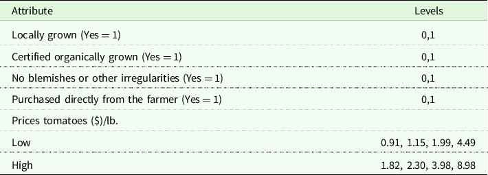
A survey and choice experiment were designed to elicit consumer preferences for local and organic produce in Northern New England and included three sections: “Introduction” section familiarized the consumer with the products being valued and gathered information on attribute preferences for the target population; “Anchoring Effects and the Role of Information” section presented the choice experiment and a set of related follow-up questions; and “Experimental Design and Data Summary” section gathered a set of socio-economic indicators from each of the survey respondents. For the empirical experiment concerned with testing for anchoring bias and the effectiveness of information scripts on mitigating such bias in a discrete choice framework, the responses to a study collecting individuals’ preferences for local and organic agriculture in Northern New England were analyzed. Here, an online survey is used to compare a treatment group, i.e. anchoring information (INFO) with a neutral control group, i.e. no anchoring information (NoINFO). Formally, the test was carried out by using a split-sample design, in which the full sample was split along two dimensions: price vector (Low/High) and anchoring information exposure (NoINFO/INFO). The price-vector dimension split the sample according to the level of the price attribute presented for each choice set, where respondents exposed to the high price split were presented with prices double that of those faced with the low price split, as shown in Table 1.
Table 1. Attributes and attribute levels in choice experiment survey
Respondents exposed to survey versions with the anchoring information (INFO) were presented with an identical set of survey questions, but the choice experiment portion of the survey was prefaced with a short script describing the issue of anchoring bias in stated preference valuation techniques. The information script presented to the respondents was as follows:
Experience from previous similar surveys is that in uncertain and hypothetical situations, people often base their responses to questions on easily accessible information. That is, people often anchor their responses to a question based on the first piece of information they see, even though this information might be contrary to their actions in a similar, non-hypothetical situation. Throughout the following section, keep in mind that the price presented for each bundle does not necessarily reflect the actual value you might see in a marketplace. And more importantly, do not consider the proposed bundle prices as the “true” value of the bundle, particularly as they relate to your preferences for the vegetable.Footnote 3
Based on qualitative information gathered from focus groups of consumers and producers in the region, tomatoes are presented in the choice experiment as being composed of five product attributes, summarized in Table 1 below. The first two attributes are indicators of whether the produce were grown locally or through certified organic practices.Footnote 4 Another indicator describing the method of purchase (i.e. directly from farmers or indirectly from other markets) was included as an attribute and is expected to capture preferences around purchasing convenience, as well as social capital considerations.Footnote 5 Further, Bond et al. (Reference Bond, Thilmany and Keeling-Bond2008) and Brown and Miller (Reference Brown and Miller2008) suggest that freshness and quality are the most important attributes for consumers who purchase produce. Thus, to capture the fact that consumers are often forced to make quality judgments based on appearance alone, an attribute indicating if the produce has visual blemishes was included in the experimental design. Finally, price is included to obtain the willingness to pay estimates for each of the non-price attributes.
Among the five attributes detailed in Table 1, four attributes have two levels (Yes/No) and the price attribute takes on four levels. As shown in Figure 1, consumers are asked to make a choice over three bundles of produce, two of which are hypothetical bundles proposed in the choice set, and the third representing their current purchasing habits. An orthogonal main effects design was conducted using the JMP software suite to ensure no interactions between the attributes, as each level of one factor occurs with each level of another factor with equal or at least proportional frequencies. Results from this design technique reduced 24 x 4 = 64 possible combinations into eight combinations of attributes, which are then split into four versions of the survey with two combinations in each version. Therefore, information is gathered on two choice sets over varying tomatoes for each respondent.
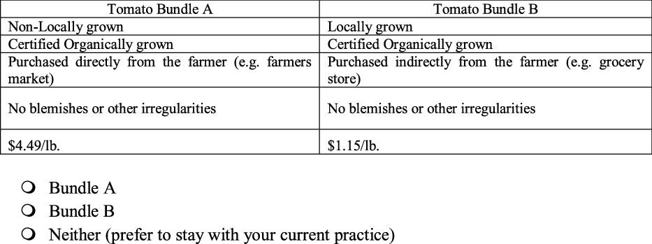
Figure 1. Example of choice experiment survey bundle.
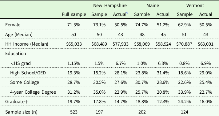
The four versions of the survey are divided into four subsamples: (1) LP/NoINFO; (2) HP/NoINFO; (3)LP/INFO; and (4) HP/INFO, for a total of 16 versions of the survey. The survey questionnaires were created and distributed via the Qualtrics Survey Research Suite, through which a quota-based approach was used to sample from an online panel, where respondents were screened and filtered according to three criteria: (1) at least 18 years old; (2) the households primary food shopper; and (3) a resident of New Hampshire, Maine, or Vermont. Additionally, respondents who failed a “focus test” were also removed from the analysis. Footnote 6 Details on the development of the survey instrument and the policy background can be found in Pyburn et al. (Reference Pyburn, Puzacke, Halstead and Huang2016). Data collection was handled in 2017 by the Marketing Systems GroupFootnote 7 , who controls an online panel consisting of members of the general United States public. Respondents were invited via email and due to the sampling scheme, it is not possible to calculate a standard response rate as a quota-based sampling frame was employed. After clearing incomplete responses and non-compliers, 523 respondents remain in the final sample, consisting of 197 respondents from New Hampshire, 202 from Maine, and 124 from Vermont. The proportions of respondents chosen from each state were based on share of population across the three states.
Table 2 presents demographic summary statistics of survey respondents and their associated populations for comparison, by state. Across the full sample, 71.3% of respondents are female, though this percentage is somewhat lower in Vermont (62.9%) and represents a larger proportion of females than their population average of about 50%. The mean age across the sample is about 50 years old, with a standard deviation of 16.3, indicating that the sample has a broad coverage of age groups used in estimation and is roughly consistent with population averages, though the sample in New Hampshire and Vermont are about 7 years older than their population average. The median annual household income across the sample is $65,033, where this average is higher in VT ($70,887) and lower in ME ($58,069), and most likely found in NH ($68,5489). In terms of educational attainment, 79.6% of respondents have at least some college education and is slightly higher than each of the three states averages.
Table 2. Summary statistics of respondent characteristics by state
Modeling framework and specification
To test for the presence of anchoring effects and whether anchoring information treatments were an effective anchoring mitigation technique, a set of discrete choice models are used to analyze and compare the preference structures and WTP estimates across each of the treatment and control groups for the product. The discrete-choice random utility (RUM) framework (McFadden Reference McFadden1973) is used to analyze respondents’ choices among different bundle alternatives.
Equation 2 below represents the utility function of decision maker i over choice alternative j. It is assumed to contain both a deterministic and random component. The deterministic component ( $\beta \prime{x_{ij}})$
is usually assumed to be a linear function of the choice attributes, the price of the choice, and individual characteristics, which are included through their interactions with an alternative-specific constant and
$\beta \prime{x_{ij}})$
is usually assumed to be a linear function of the choice attributes, the price of the choice, and individual characteristics, which are included through their interactions with an alternative-specific constant and $\beta $
is a vector of coefficients assumed constant across individuals and choice alternatives.Footnote
8
The random component (
$\beta $
is a vector of coefficients assumed constant across individuals and choice alternatives.Footnote
8
The random component ( ${\varepsilon _{ij}})$
is included as an error term and is assumed to be randomly distributed.
${\varepsilon _{ij}})$
is included as an error term and is assumed to be randomly distributed.
 $${U_{ij}} = \beta ^{\prime}{x_{ij}} + {\varepsilon _{ij}}$$
A rational decision maker chooses the alternative that yields the highest utility, such that the probability of decision maker i choosing alternative j over other alternatives k is
 $${\pi _{ij}} = {\rm{Pr}}(\beta ^{\prime}{x_{ij\;}} + {\varepsilon _{ij}} \gt \beta ^{\prime}{x_{ik\;}} + {\varepsilon _{ik}})\;\;\forall j \ne k$$
Assumptions about the distribution of the error term in Eq. 3 lead to different types of discrete choice models. For example, if we assume the error term follows an i.i.d. Type I extreme value distribution, the conditional logit model arises. This type of model is widely used in the choice-modeling literature. The benefits of using the conditional logit model are in its operational simplicity, whereas the costs are in: (1) its inability to account for preference heterogeneity across decision-makers; and (2) its restrictive IIA assumption.
Within this model, the conditional probability that decision maker i chooses alternative j can be expressed as
 $${\pi _{ij}} = \;{{{\rm{exp}}\left( {\beta ^{\prime} {x_{ij}}} \right)} \over {\sum\nolimits_{j = 1}^J {{\rm{exp}}} \left( {\beta ^{\prime} {x_{ij}}} \right)}}$$
where J is the maximum number of choice alternatives faced by decision maker i. The log-likelihood function of the choice responses made by n decision-makers can be expressed as
 $$L = \;\mathop \sum \nolimits_{i = 1}^n [{y_{i1}}\log \left( {{\pi _{i1}}} \right) + {y_{i2}}\log \left( {{\pi _{i2}}} \right) + \ldots + {y_{iJ}}\log \left( {{\pi _{iJ}}} \right)]\;$$
where $n$
is the total number of decision makers, and
$n$
is the total number of decision makers, and ${y_{i1}} = 1$
if decision-maker i chooses alternative j, and
${y_{i1}} = 1$
if decision-maker i chooses alternative j, and ${y_{i1}} = 0$
otherwise.
${y_{i1}} = 0$
otherwise.
For this analysis, the mixed logit modeling approach is used. (Train Reference Train2003) This class of models allows for individual preference heterogeneity and relaxes the restrictive IIA assumption by allowing one or more of the parameters in the model to be randomly distributed (Revelt and Train Reference Revelt and Train1998). Here, if we assume $\beta $
to be randomly distributed with density
$\beta $
to be randomly distributed with density $f\left( {{\beta _i}{\rm{|}}\theta } \right)$
where
$f\left( {{\beta _i}{\rm{|}}\theta } \right)$
where $\theta $
represents the true parameters of the distribution, the unconditional probability of decision-maker i choosing alternative j is the conditional probability of (6) integrated over the distribution of
$\theta $
represents the true parameters of the distribution, the unconditional probability of decision-maker i choosing alternative j is the conditional probability of (6) integrated over the distribution of $\beta $
, or
$\beta $
, or
 $${\pi _{ij}^*} = \;{{{\rm{exp}}\left( {\beta ^{\prime}_i{x_{ij}}} \right)} \over {\mathop \sum \nolimits_{j = 1}^J {\rm{exp}}\left( {\beta ^{\prime}_i{x_{ij}}} \right)}}\;f\left( {{\beta _i}{\rm{|}}\theta } \right)\;d{\beta _i}\;\;$$
Since the integral in (6) cannot be evaluated analytically, exact maximum likelihood estimation is not possible. Instead, the probability is approximated through simulation. The simulated log likelihood is given by
 $$SLL\left( \theta \right) = \;\sum\limits_{n = 1}^N {{\rm{ln}}} [{1 \over R}\sum\nolimits_{r = 1}^R {\pi _{ij}^*} \left( {{\beta ^r}} \right)]$$
where R is the number of replications and ${\beta ^r}$
is the r-th draw from
${\beta ^r}$
is the r-th draw from $f\left( {{\beta _i}{\rm{|}}\theta } \right)$
.
$f\left( {{\beta _i}{\rm{|}}\theta } \right)$
.
Within this framework, welfare measures, i.e. marginal willingness to pay (WTP), are calculated according to Eq. 1, in which the non-monetary coefficients of interest (i.e. local, organic, etc…) are divided by the price coefficient and is carried out using the wtp command in Stata 13.1, the details of which can be found in Hole (Reference Hole2007a).
To test for anchoring effects, we run the following specification separately for each price split group who were not exposed to anchoring information (NoINFO), specifically,
 $${U_{ij|LP,NoINFO}} = f({P_{ij}},{D_{ij}},\;S{Q_i},{Y_i}*S{Q_i},{e_{ij}}|\beta )$$
and
 $${U_{ij|HP,NoINFO}} = f({P_{ij}},{D_{ij}},\;S{Q_i},{Y_i}*S{Q_i},{e_{ij}}|\alpha )$$
where P
ij
indicates the price of alternative j presented to individual i, D
ij
is a series of indicator variables identifying all of the choice alternative attributes, SQ
ij
represents the status quo, or current purchasing behavior of individual i, and (Y
i
*SQ
i
) which represents a set of interactions between the status quo alternative and other individual characteristics, including sex, income, and education, state-level dummy indicators, and a measure of purchasing experience
Footnote 10
, and finally $\beta $
and
$\beta $
and $\alpha $
represent the set of parameters that define each group. The test for anchoring effects is carried out by testing the equivalence of
$\alpha $
represent the set of parameters that define each group. The test for anchoring effects is carried out by testing the equivalence of $\beta $
and
$\beta $
and $\alpha $
across the two models via a likelihood ratio test developed in Swait and Louviere (1993), where the null hypothesis is
$\alpha $
across the two models via a likelihood ratio test developed in Swait and Louviere (1993), where the null hypothesis is $H_0^{Anch1}:$ $\beta $
=
$\beta $
= $\alpha $
, or that parameter estimates are equivalent across the two groups. Within this specification, the binary attributes of interest (i.e. local, organic, indirect, and non-blemish) are assumed random and uncorrelated, each following a normal distribution.Footnote
11
Once preference estimates are obtained and if
$\alpha $
, or that parameter estimates are equivalent across the two groups. Within this specification, the binary attributes of interest (i.e. local, organic, indirect, and non-blemish) are assumed random and uncorrelated, each following a normal distribution.Footnote
11
Once preference estimates are obtained and if $H_0^{Anch1}$
is rejected, we also test for anchoring effects by differences in attribute-level marginal willingness-to-pay estimates across the two groups. The null hypothesis here is
$H_0^{Anch1}$
is rejected, we also test for anchoring effects by differences in attribute-level marginal willingness-to-pay estimates across the two groups. The null hypothesis here is $H_0^{Anch2}\;:WTP_j^{LP|NoINFO} = WTP_j^{HP|NoINFO}$
, where j represents the attribute of interest. Failure to reject
$H_0^{Anch2}\;:WTP_j^{LP|NoINFO} = WTP_j^{HP|NoINFO}$
, where j represents the attribute of interest. Failure to reject $H_0^{Anch1}$
or
$H_0^{Anch1}$
or $H_0^{Anch2}$
would suggest that price anchoring effects are not present in this choice experiment.
$H_0^{Anch2}$
would suggest that price anchoring effects are not present in this choice experiment.
Lastly, to test the effectiveness of anchoring information (INFO) in mitigating anchoring effects relative to the neutral no information control (NoINFO), we take a similar approach as outlined above, but only estimate for those exposed to the information prompts. Specifically, we estimate
 $${U_{ij|LP,INFO}} = f({P_{ij}},{D_{ij}},\;S{Q_i},{Y_i}*S{Q_i},{e_{ij}}|\gamma )$$
and
 $${U_{ij|HP,INFO}} = f({P_{ij}},{D_{ij}},\;S{Q_i},{Y_i}*S{Q_i},{e_{ij}}|\tau )$$
and carry out similar likelihood ratio tests for data pooling, where the null hypotheses now can be represented by $H_0^{INFO1}:$ $\gamma $
=
$\gamma $
= $\tau $
and
$\tau $
and $H_2^{INFO2}\;:WTP_j^{LP|INFO} = WTP_j^{HP|INFO}$
. Here, failure to reject either
$H_2^{INFO2}\;:WTP_j^{LP|INFO} = WTP_j^{HP|INFO}$
. Here, failure to reject either $H_0^{INFO1}$
or
$H_0^{INFO1}$
or $H_0^{INFO2}$
would suggest that the information intervention completely eliminated any anchoring effects. On the other hand, if
$H_0^{INFO2}$
would suggest that the information intervention completely eliminated any anchoring effects. On the other hand, if $H_0^{INFO1}$
or
$H_0^{INFO1}$
or $H_0^{INFO2}$
are rejected, then we test for mitigating effects of information by developing a measure of the difference in anchoring both before and after exposure to anchoring information, represented by
$H_0^{INFO2}$
are rejected, then we test for mitigating effects of information by developing a measure of the difference in anchoring both before and after exposure to anchoring information, represented by
 $$DIFF = \left( {WTP_{j,k}^{INFO|HP} - \;WTP_{j,k}^{INFO|LP}} \right) - \left( {WTP_{j,k}^{NoINFO|HP} - \;WTP_{j,k}^{NoINFO|LP}} \right).$$
Here, the null hypothesis is $H_0^{INFO3}\;:\;DIFF = 0$
, or that anchoring effects before and after the information exposure are the same. If
$H_0^{INFO3}\;:\;DIFF = 0$
, or that anchoring effects before and after the information exposure are the same. If $H_0^{INFO3}$
is rejected and
$H_0^{INFO3}$
is rejected and $DIFF \lt 0$
, this would indicate that information treatment instead had a mitigating effect on price anchoring. Finally, if
$DIFF \lt 0$
, this would indicate that information treatment instead had a mitigating effect on price anchoring. Finally, if $H_0^{INFO3}$
is rejected and
$H_0^{INFO3}$
is rejected and $DIFF \gt 0$
, the anchoring intervention had a perverse effect on anchoring behavior.
$DIFF \gt 0$
, the anchoring intervention had a perverse effect on anchoring behavior.
If anchoring information did indeed have an effect on the level of anchoring, we can expect one of two things to happen. First, for those exposed to the low price sample, information treatment would reduce the price sensitivity of those consumers and for those exposed to the high price sample, we can expect just the opposite, in that price sensitivity for these individuals increases. That is to say, anchoring information can have an effect on price sensitivity for either group, but as the prices presented to the low price sample more closely align with actual market prices, we would expect greater effects of information in the high price sample.
All models based upon the above procedure are estimated in Stata (StataCorp 2013), using the mixlogit (Hole Reference Hole2007b) command, which is simulated through Halton draws using 1000 replications.
Results
The results presented in this section detail summary measures of respondent choice frequencies, highlight the presence of anchoring in respondent choices, and uncover the mitigating effects of anchoring-specific information through both preferences and derived welfare estimates.
Respondent choice frequencies
As a first step in this analysis, we investigate whether respondent choice frequencies are variant to price scale and anchoring information exposure. The frequencies of respondents’ selection of each alternative under the price and information treatments are summarized in Table 3. As theory would suggest, we can expect to see acceptance rates decrease as price increases, i.e. Price Level 1 to Price Level 4, and this mostly holds across each of the price scales and information treatments. Overall, across each of the price vectors and information treatments, we find the lowest price level is chosen more frequently than the highest price level; the only deviations from this rational action occur at price levels one level away from each other and the difference between these choice frequencies are not statistically significant. Additionally, looking at these choice frequencies across the two price groups, we find the only statistically significant difference in choice frequency at the highest price level for those not exposed to the anchoring information treatment. Specifically, those exposed to low prices were likely to choose the highest price level ($4.99/lb.) 6.1% of the time, while those exposed to high prices were likely to choose the highest price level ($8.98/lb.) 1.1% of the time. This difference in choice frequency at the highest price level does not hold for those exposed to the information intervention, suggesting some effects of the intervention on the respondents choice process.
Table 3. Respondents’ option selection frequency under two price levels in choice experiment
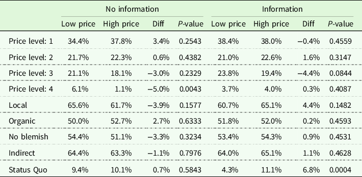
Notes: Diff is calculated as the difference between the High Price and Low Price groups. P-values were calculated using a two-sample t-test assuming unequal variances across the two groups.
In terms of the other choice attributes, some patterns begin to emerge across price vectors and information treatments. Specifically, we find that respondents choose at higher rates tomatoes that are locally produced, organic, non-blemished in appearance. We also find a clear preference for indirect purchasing (i.e. from a grocery store), regardless of price scale and information exposure. Further, we find that choice of the status quo option increased for those exposed to the high price scale, relative to the low, though this difference is only significant for those exposed to the information treatment. This is a result we expected to find and confirms that it is likely that status quo effects will be larger for respondents presented with the high price scale survey split (Samuelson and Zeckhauser Reference Samuelson and Zeckhauser1988).
Presence of anchoring
Table 4 presents mixed logit model parameter estimates from the choice experiment for respondents exposed to high and low price splits without an anchoring information treatment, as well as pooled estimates across the two sample splits, for a total of three models. Across all three models the coefficient of the price attribute is well-behaved, in that a higher price reduces the chance of an alternative being chosen. Further, we find the absolute value of the price coefficient is lower for the high-price sample, suggesting lower sensitivity to price when respondents are exposed to higher price levels, consistent with diminishing marginal (dis)utility on price. The coefficients on the local and indirect attributes are positive and significant at the 99% level, suggesting that consumers prefer tomatoes that are grown locally and would prefer to purchase tomatoes through indirect venues, such as through a grocery store or supermarket.
Table 4. Mixed logit estimates for choice experiment before information treatment, by price level
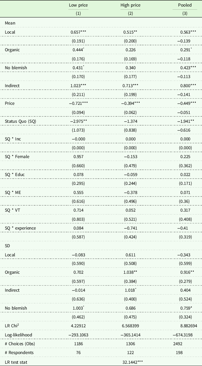
Notes: Numbers in parentheses are standard errors.
*, **, ***Indicate statistical significance at the 0.10, 0.05, and 0.01 levels, respectively.
Bolded LR Test Stat indicates statistic is significant at the 0.01 level or lower.
Likelihood ratio tests were used to test whether changing the price level led to different parameter estimates in the choice experiment and are presented in the final row of Table 4. The restricted models are pooled across the high and low price vectors, while the unrestricted models (Columns 1 and 2) are split by high and low price vector. The null hypothesis for these tests is to not reject data pooling, i.e. consumers across the two price splits have the same set of preferences across product attributes and all possible interactions between attributes. Here, rejecting the null hypothesis would suggest that respondents’ preferences for product attributes were sensitive to the price vector presented. The test statistic is presented in the bottom row of each of the tables. The critical chi-square value with 16 degrees of freedom at the 95% confidence level is 26.3. The null hypothesis is rejected in this case, showing that respondents’ preferences for tomatoes were affected by the price vector presented in the choice experiment, suggesting the presence of price anchoring effects among respondent choices.
Mean marginal willingness-to-pay (WTP) for each of the attributes is presented in Table 5 and their accompanying confidence intervals are calculated using the Krinsky-Robb parametric bootstrap technique following the wtpcikr command in Stata 13.1. Here, Columns (1) and (2) represent WTP estimates from the low price and high price split, respectively, and Column (3) is the difference in WTP estimates between those same splits.
Table 5. Evidence of anchoring effects: effects of doubled price level in choice experiment on difference in mean marginal WTP ($/pound)
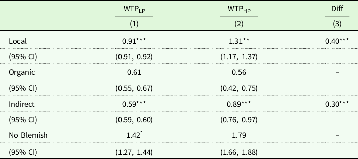
Notes: WTPLC and WTPHC are predicted WTP from respondents who participated in choice experiment with low price (LP) and high price (HP) levels. Diff are differences between respondents predicted WTP between the different price levels: Diff = WTPHC – WTPLC.
*, **, ***Indicate statistical significance at the 0.10, 0.05, and 0.01 levels, respectively.
Diff only shown for those WTP figures that are significant at the 0.01 level.
Overall, doubling the price level in the choice experiment substantially increased respondents marginal WTP for most attributes of tomatoes, thus consistent with the hypothesis of an anchoring effect. Specifically, holding all else constant, welfare estimates on the local and indirect attributes for those respondents presented with the high price sample increased by $0.40 and $0.30 per pound, respectively. Footnote 12 These increases in marginal WTP represent anchoring effects on the magnitude of 43.9% and 50.8% across these two attributes, respectively, and are significant at the 99% level.
Effects of the anchoring information intervention
A similar approach was used to test for potential mitigating effects of the anchoring information intervention. Specifically, Table 6 presents likelihood ratio tests to determine if exposure to the information intervention had a differential effect on model parameter estimates. Here, the restricted model is with pooled data from the choice experiment with both the information treatment (INFO) and no information control (NoINFO), while the unrestricted models are the separate models from the choice experiment, one with the INFO treatment and the other with NoINFO control. The null hypothesis here is, again, failure to reject data pooling between the two samples and ejection of the null hypothesis in this respect would suggest that the information intervention affected respondents’ choices across price vectors. The critical chi-square value with 14 degrees of freedom at the 95% confidence level is 26.296. Therefore, as is shown in the bottom row of Table 6, the null hypothesis of equal parameters is not rejected for each price split, providing evidence that the information intervention did not completely eliminate the anchoring effects discussed above. It is important to note that this does not rule out potential mitigating effects of the information intervention, as the differences in preferences across the models are primarily among the coefficient on price, and not coefficients across all of the model parameters.
Table 6. Mixed logit estimates for choice experiment with information treatment (INFO) and no information control (NoINFO), by high price and low price levels
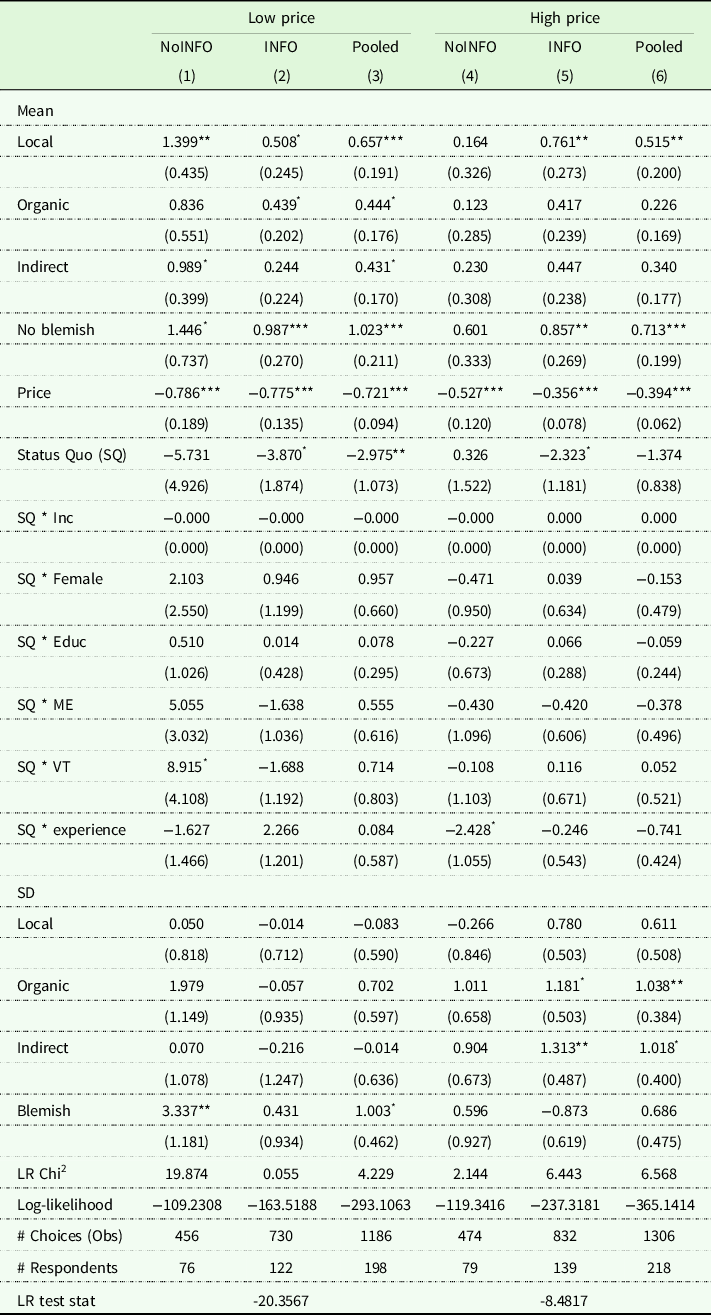
Notes: Numbers in parentheses are standard errors.
*, **, ***Indicate statistical significance at the 0.10, 0.05, and 0.01 levels, respectively.
Bolded LR Test Stat indicates statistic is significant at the 0.01 level or lower.
To understand if the information intervention had a mitigating effect on anchoring, we follow a similar procedure as above by testing for pooling across the two price vectors for those only exposed to the information intervention. Additionally, as there seemed to be some evidence of a potential treatment effect of exposure to information on the price attribute, an information interaction term (INFO) was included across each of these models, here interacting a dummy identifying exposure to information with the price attribute and the status quo option only. Results for these models are presented in Table 7. The interactions between the price and status quo with the information dummy variable are insignificant, suggesting that exposure to information did not have a significant effect on the choice of price or the status quo. Additionally, we run a pooling procedure as detailed above and reject the null hypothesis of data pooling across the high and low price sample groups, again implying that the information intervention failed to eliminate anchoring effects.
Table 7. Mixed logit estimates for choice experiment with high price and low price levels incl. INFO interactions, by price level
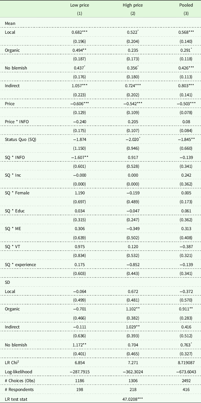
Notes: Numbers in parentheses are standard errors.
*, **, ***Indicate statistical significance at the 0.10, 0.05, and 0.01 levels, respectively.
Bolded LR Test Stat indicates statistic is significant at the 0.01 level or lower.
We can additionally test for the mitigating effects of information exposure on welfare estimates. Table 8 below presents mean marginal WTP estimates across price-vector after controlling for information treatment exposure and are calculated based on parameter estimates from Table 7. If anchoring-specific information prompts were to completely eliminate anchoring effects, we would expect to see no significant difference in the WTP estimates between each of the high and low price splits after exposure and is not something we expect to find based upon the pooling procedures above. Overall, we still find significant differences between these two price splits, suggesting that exposure to information was insufficient at eliminating associated price anchoring effects. Rather, we find that exposure to information had heterogeneous impacts on WTP estimates. In particular, for those exposed to the low price split, WTP estimates increased for each attribute of tomatoes after exposure to anchoring information. Conversely, for those exposed to the high price split, WTP estimates decreased across attributes after exposure to the same intervention.
Table 8. Evidence of anchoring after information exposure: effects of doubled price level after controlling for exposure to anchoring information in choice experiment on difference in mean marginal WTP ($/pound), for mixed logit model
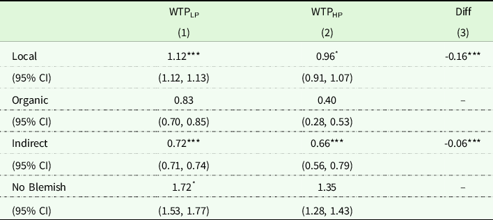
Notes: WTPLP and WTPHP are predicted WTP from respondents who participated in choice experiment with low price (LP) and high price (HP) levels. Diff are differences between respondents predicted WTP between the different price levels: Diff = WTPHP – WTPLP.
*, **, ***Indicate statistical significance at the 0.10, 0.05, and 0.01 levels, respectively.
Diff only shown for those WTP figures that are significant at the 0.01 level.
Though the results detailed above suggest that anchoring-specific information prompts were unable to completely eliminate price anchoring in this choice experiment, Table 9 presents evidence that it was successful at mitigating anchoring effects. Columns (1) and (2) of Table 9 show the differences in WTP estimates between high and low price splits and the DIFF column shows the change in those differences after exposure to information, and can be interpreted as a reduction in anchoring effects induced by the information treatment. Here, negative values would suggest a reduction in anchoring effects and positive values an increase. We calculate the overall difference in anchoring by subtracting the absolute value of the difference for those not exposed to the intervention from the difference in the value for those who were exposed. As is shown in Table 9, the information intervention is associated with a reduction in anchoring effects of 60% and 80% on the local and indirect attributes, respectively, and these reductions in anchoring are primarily driven by the interventions impact on the price attribute.
Table 9. Reduction in anchoring effects before and after information: differential effects of doubled price level before and after controlling for exposure to information in choice experiment on mean marginal WTP ($/pound)
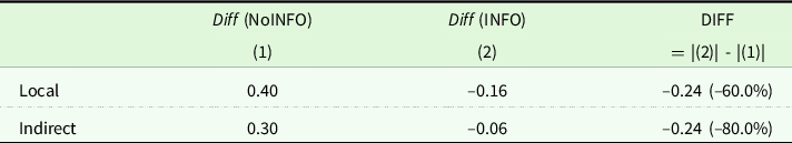
Notes: Values presented are WTP estimates from respondents who participated in choice experiment with low price (LP) and high price (HP) levels.
Diff are differences in simulated WTP between the different price levels, by anchoring information treatment: Diff = WTPHP – WTPLP.
DIFF represents differences in the differences between price split and information treatment and can be interpreted as a reduction in anchoring effects induced by the information treatment.
Conclusions and discussion
This analysis reveals a conclusion that is novel, though perhaps unsurprising: ex ante treatments in the form of “information” aimed at affecting price sensitivity in choice experiments have potential to mitigate price anchoring effects. Specifically, we find that using a split sample experimental design, doubling the price vector in this choice experiment increases marginal willingness-to-pay from 44 to 51% and that exposure to anchoring-specific information interventions decreases these anchoring effects between 60 and 80%. It is worth noting that the convergence of the HighPrice/INFO and LowPrice/NoINFO group welfare estimates is not due exclusively to changes in the price coefficient of the anchoring information treatment groups. When we refer to the “effect of information”, we are not referring to the price coefficient explicitly. Rather, we interpret the information effect as the wedge that forms in the welfare estimates derived from both the treatment and control groups, which can be due to differences in the price coefficient or other attribute coefficients from which the welfare estimate is calculated.
Methodologically, the results presented here have important implications for future choice experiment design. Choice experiments come in many forms, and many decisions can impact researchers’ ability to accurately elicit preferences. Each decision is not made in a vacuum; instead the appropriateness of one choice depends on other choices, which underlies the importance of thorough pretesting in the survey design process. Our analysis is not the first to suggest that the effects of price anchoring may pose significant issues for choice experiment design and context. Our analysis is, though, the first to provide evidence that ex ante information interventions have the potential to mitigate some of these anchoring effects in online choice exercises.
It is also possible that the nature of the products being considered (i.e. private vs. public goods) may be driving some of these results, though it is a priori unclear in which direction. For example, the price anchoring effects found in this study are smaller than anchoring effects found in other similar studies that examine public goods (Carlsson and Martinsson Reference Carlsson and Martinsson2007). A potential explanation here could be in terms of variations in experience, through which individuals are thought to learn their preferences after a greater experience with the product, or in the choice experiment setting, over repeated choices. Given that respondents have actual experience in a market setting purchasing tomatoes, respondent price sensitivity might be lower in this private good setting. Also, for this reason, information intervention effects might be smaller in this setting as this information is expected to have more significant impact on respondents of lower levels of certainty over their preferences for the products in question. Further research is required to test the differences in information interventions between public and private goods and across respondents of varying experience.
In the application of this paper, we investigate Northern New England residents’ preferences for fresh tomatoes. Overall, our estimates reveal that consumers are willing to pay a substantial price premium for locally grown tomatoes, in the range of $0.96–$1.12 per pound, whereas they are not willing to pay a price premium for organically grown tomatoes. These results are similar to those found in Thilmany et al. (Reference Thilmany, Bond and Bond2008) and Werner et al. (2018). Together, these studies lend support to farmers and policy makers decisions over the production of locally grown fresh produce. Comparing the premiums for locally and organically grown attributes, Northern New England consumers tend to consider the locally grown attribute as a more important feature when purchasing produce. These results may offer some guidance for farmers regarding growing practice and farm land use as regional coalitions support local agriculture expansion in the Northeast (McCabe and Burke Reference McCabe and Burke2012).
Overall, these results draw conclusions that are important for the stated-preference valuation literature and lend themselves to an active research agenda moving forward. Specifically, interventions that test variations of anchoring-specific information interventions and reiterate the main assertions of the information script repeatedly through the choice experiment may serve as an additional catalyst for price anchoring mitigation. Our hope is that this work encourages researchers to be mindful of the effects of the choice of price vectors in the choice experiment setting and to build short anchoring information interventions into future research designs. This approach is of relatively low cost and is crucial to furthering the field’s understanding of how different design decisions impact response and preference elicitation in stated preference surveys.
Supplementary material
To view supplementary material for this article, please visit https://doi.org/10.1017/age.2022.10
Acknowledgements
The authors would like to acknowledge Samantha Werner, Maria Pyburn, and Wei Shi for their initial efforts in developing the survey instrument. Additionally, we would like to thank Bruce Pfeiffer and participants from the 2018 Workshop on Non-Market Valuation for their helpful comments on this work.
Author Contributions
All authors contributed equally to the development of this paper.
Funding statement
This research was supported by the National Institutes for Food and Agriculture (NIFA), U.S. Department of Agriculture, and by the New Hampshire Agricultural Experiment Station under Multistate Project 1749. This is Scientific Contribution #2746.
Competing interests
None.
Ethical Standards
Informed consent was obtained from all individual participants involved in the study.


 Open access