

The U.S. dairy industry has gone through significant structural changes in the last few decades and toward ever larger operations. The total output of milk has increased by 33 percent from 150.8 billion pounds in 1992 to 200.6 billion pounds in 2012, despite a 4.7 percent decline in the total stock of dairy cows. The innovations in milking, animal housing, improved animal care, and advances in dairy genetics have allowed some dairies to expand rapidly, whereas many dairies that remained at small scales chose to leave the industry (McDonald et al., Reference McDonald, O'Donoghue, McBride, Nehring, Sandretto and Mosheim2007). The total number of dairy farms (with 20 or more cows) has declined by about 60 percent during 1992–2012, down to about 44,000 farms (USDA-NASS, 2012).
Amid the structural change, a movement to advance the ancient practice of grazing milk cows has emerged. Management-intensive grazing (MIG), or rotational grazing, as it is known in the dairy science literature, is a low-input, low-output dairy system with the potential to become a viable alternative to the small- to medium-scale conventional confinement operations. Compared to confinement dairies, MIG dairies rely less on feed purchases and mechanically harvested feed, two factors that help reduce the environmental footprint due to reduced soil erosion (DiGiacomo et al., Reference DiGiacomo, Iremonger, Kemp, van Schaik and Murray2001) and phosphorous run-off (Bishop et al. Reference Bishop, Hively, Stedinger, Rafferty, Lojpersberger and Bloomfield2005). MIG dairies have lower capital requirements, also appealing for new entrants. The challenge for MIG dairies, on the other hand, is to meet the nutritional requirements of the herd. The producer must adhere to strict pasture management, primarily by rotating the animals among partitioned pasture paddocks on a daily basis to fully use the regenerative potential of pastures. Milk production per cow, along with the use of conventional inputs, substantially declines under MIG practices. Therefore, the economic competitiveness of MIG dairies depends on the relative decline in inputs to the decline in milk production, the relative prices of milk and production inputs, and the efficiency of the operation. Some studies suggest MIG dairies can be as competitive as confinement operations at relatively small scales (Elbehri and Ford Reference Elbehri and Ford1995, Dartt et al. Reference Dartt, Lloyd, Radke, Black and Kaneene1999, Gloy, Tauer, and Knoblauch Reference Gloy, Tauer and Knoblauch2002, Hanson et al. Reference Hanson, Johnson, Lichtenberg and Minegishi2013).Footnote 1
Whether it is a confinement or a MIG operation, the economic viability of most dairies likely depends on whether they can compete against a growing number of large-scale confinement operations. So far, the evidence that economies of scale are the main drivers of consolidating milk production is mixed; some studies found increasing returns to scale in dairy production (Tauer and Mishra Reference Tauer and Mishra2006, Kumbhakar, Tsionas and Sipilinen Reference Kumbhakar, Tsionas and Sipilinen2009, Mosheim and Lovell Reference Mosheim and Lovell2009, Nehring et al. Reference Nehring, Gillespie, Sandretto and Hallahan2009),Footnote 2 while others found otherwise (Byma and Tauer Reference Byma and Tauer2010, Cabrera, Solís and del Corral Reference Cabrera, Solís and del Corral2010, Mayen, Balagtas and Alexander, Reference Mayen, Balagtas and Alexander2010, Mukherjee, Bravo-Ureta and De Vries Reference Mukherjee, Bravo-Ureta and De Vries2013, Key and Sneeringer, Reference Key and Sneeringer2014). Nevertheless, the analysis of over 1500 operations with 500 or more cows by Nehring et al. (Reference Nehring, Gillespie, Sandretto and Hallahan2009) presents the most compelling evidence of scale economies to this date. Greater clarity may be achieved by the research into the relationship between the emergence of large-scale confinement operations in certain production areas and the factors contributing to rapid dairy expansions such as the abundance of land, feed, and labor (Blayney Reference Blayney2002, McBride and Green Reference McBride and Green2009). If producers in certain regions are at a disadvantage in exploiting scale economies, the success of large-scale operations in places such as California, Washington, Idaho, New Mexico, and Florida would not be easily replicated elsewhere. This is particularly important for traditional dairy communities in the Upper Midwest and the Northeast, where many small- and medium-scale dairies have disappeared, but there has not been a dramatic expansion in large-scale confinement operations.
This article contributes to the ongoing discussions of structural change in the U.S. dairy industry by providing an analysis of technical change for confinement and MIG dairies that operated in Maryland during 1995–2009. The rate of technical change is a key indicator for the fundamental performance of the industry, and the comparison of this rate provides implications for the mid-term prospects of the two dairy systems. Discussion of the affects of specific technological innovations that transformed dairy operations is beyond the scope of this article. Instead, our analysis is centered on the estimation of a technological frontier and its intertemporal shift. Building on the Malmquist Productivity Index (MPI) decomposition using data envelopment analysis (DEA; Färe et al. Reference Färe, Grosskopf, Norris and Zhang1994), we devise a novel approach to decompositional measures that can be estimated from unbalanced panel data. Our estimation model, a variant of two-stage DEA analysis, also accounts for some noninput factors that may influence production outcomes. The article proceeds as follows: Section 2 describes the methodology, Section 3 presents the data and empirical analyses, and Section 4 concludes the study.
2. Model
2.1. Measurement of Technical Change
Consider a model of milk production y
it
in which producer $i \in {\rm {\opf I}} = \{ 1,..,I\} $
chooses L-dimensional inputs
x
it
in time
$i \in {\rm {\opf I}} = \{ 1,..,I\} $
chooses L-dimensional inputs
x
it
in time $t \in {\rm {\opf T}} = \{ 1,...,T\} $
. A canonical representation of that model is
$t \in {\rm {\opf T}} = \{ 1,...,T\} $
. A canonical representation of that model is
 $$y_{it} = f_t\lpar {\bi x}_{it}\rpar \cdot exp\lpar\!-\!u_{it} + v_{it}\rpar $$
where $f_t:{\rm {\opf R}}_ + ^L \to {\rm {\opf R}}_ + $
is the technological frontier in time t, exp(−u
it
) is multiplicative technical efficiency TE
it
∈ (0, 1], and exp(v
it
) is a random error. Our interests are to analyze intertemporal structures of the technological frontier f
t
(.) and the efficiency TE
it
.
$f_t:{\rm {\opf R}}_ + ^L \to {\rm {\opf R}}_ + $
is the technological frontier in time t, exp(−u
it
) is multiplicative technical efficiency TE
it
∈ (0, 1], and exp(v
it
) is a random error. Our interests are to analyze intertemporal structures of the technological frontier f
t
(.) and the efficiency TE
it
.
There are two major approaches to making equation (1) operational: parametric and semiparametric frontier models. In the parametric approach, the intertemporal patterns of a frontier and efficiency can be distinguished by imposing different functional assumptions. For instance, the pattern of frontier transitions may be specified as equiproportional shifts, in the forms of smooth interactions between the time variable and production inputs, or nonsmooth interactions via time-specific technological parameters. The pattern of efficiency may be modeled through a specific functional form (Battese and Coelli Reference Battese and Coelli1992, Cuesta Reference Cuesta2000), a function of non- input-output variables (Battese and Coelli Reference Battese and Coelli1995), or producer-specific effects (Schmidt and Sickles Reference Schmidt and Sickles1984, Cornwell, Schmidt and Sickles, Reference Cornwell, Schmidt and Sickles1990, Kumbhakar Reference Kumbhakar1990, Lee and Schmidt Reference Lee, Schmidt, Fried, Lovell and Schmidt1993, Karagiannis, Midmore and Tzouvelekas Reference Karagiannis, Midmore and Tzouvelekas2002, Roll Reference Roll2013). The empirical challenge is to select appropriate specifications for these patterns that are both conceptually compelling for the case at hand and compatible with the data.
In the semiparametric approach, a prominent method is MPI decomposition using DEA (Färe et al., Reference Färe, Grosskopf, Norris and Zhang1994). With its roots in the economic theory of production index numbers (e.g., Samuelson and Swamy Reference Samuelson and Swamy1974, Diewert Reference Diewert1976, Caves, Christensen and Diewert Reference Caves, Christensen and Diewert1982), the MPI decomposition offers a general framework to analyze productivity trends such as those related to technical change. The method proceeds in two stages: in the first stage a semiparametric frontier is estimated separately for each time period, and technical efficiency is measured accordingly; in the second stage are obtained the shifts of the frontier and efficiency.
One shortcoming of the method is that its deterministic estimation (i.e., exp(v it ) = 0 in (1)) can be sensitive to extreme data points and measurement errors. Another is that the method presumes a balanced panel data structure in calculating the producer-level MPI decomposition. Simply eliminating the data of producers whose observations are not available for the entire survey period can lead to biased estimates through nonrandom additions and attritions (Kerstens and Van de Woestyne, Reference Kerstens and Van de Woestyne2014).
The proposed estimation below is based on the MPI decomposition, while addressing the latter shortcoming. Specifically, to accommodate the use of unbalanced panel data, producer-level calculations of the MPI decomposition are replaced with a sample-level regression analysis of a frontier and efficiency. We derive statistical inferences based on the approach developed by Kneip, Simar and Wilson (Reference Kneip, Simar and Wilson2015) for the class of second-stage analysis estimators on DEA efficiency measures.
2.2. Two-stage Analysis of Distance Functions
Central to the MPI decomposition are the concepts of the distance between a production decision (i.e., an input-output bundle) and a technological frontier and the distance between two technological frontiers of two time periods. These distances are analyzed in two stages.
A conceptual framework is provided through the three types of distances that are derived from technical/pseudotechnical efficiency measurements. The output-oriented technical efficiency is the relative distance between decision (
x
it
, y
it
) and frontier f
t
(.), or TE
it
≡ y
it
/f
t
(
x
it
). The envelopment of f
t
(.) across time $t \in {\rm {\opf T}}$
is referred to as a metafrontier (Battese, Reference Battese2002; Battese, Rao, and O'Donnell Reference Battese, Rao and O'Donnell2004) representing the maximum attainable outputs of all time periods
$t \in {\rm {\opf T}}$
is referred to as a metafrontier (Battese, Reference Battese2002; Battese, Rao, and O'Donnell Reference Battese, Rao and O'Donnell2004) representing the maximum attainable outputs of all time periods ${\rm {\opf T}}$
, or
${\rm {\opf T}}$
, or $f^M({\bi x}) = \mathop {\max }\nolimits_{t \in {\rm {\opf T}}} \{ f_t({\bi x})\} $
. Then, two pseudotechnical efficiency measures are obtained: the technological gap ratio (TGR) defined for the relative distance between the time-t frontier and the metafrontier, or TGR
it
≡ f
t
(
x
it
)/f
M
(
x
it
), and the metatechnological efficiency (MTE), defined as the relative distance between the decision and the metafrontier, or MTE
it
≡ y
it
/f
M
(
x
it
).Footnote
3
$f^M({\bi x}) = \mathop {\max }\nolimits_{t \in {\rm {\opf T}}} \{ f_t({\bi x})\} $
. Then, two pseudotechnical efficiency measures are obtained: the technological gap ratio (TGR) defined for the relative distance between the time-t frontier and the metafrontier, or TGR
it
≡ f
t
(
x
it
)/f
M
(
x
it
), and the metatechnological efficiency (MTE), defined as the relative distance between the decision and the metafrontier, or MTE
it
≡ y
it
/f
M
(
x
it
).Footnote
3
Figure 1 illustrates these concepts in a single-input single-output case; the three distance measurements for decision ( x it , y it ) are depicted as TE it = AQ/BQ, MTE it = AQ/CQ, and TGR it = BQ/CQ. Note that MTE it = TGR it · TE it ,Footnote 4 and the intertemporal change of MTE provides a version of the MPI decomposition; Δ t ln MTE it = Δ t ln TGR it + Δ t ln TE it where Δ t ln MTE it (i.e., an intertemporal, percentage change in MTE) is a measure of productivity change, Δ t ln TGR it is a measure of technical change (TC), and Δ t ln TE it is a measure of technical efficiency change (TEC).

Figure 1. Time-specific frontiers and the meta-Frontier
In the first stage, we approximate time-t frontiers by DEA.Footnote 5 Under the nonincreasing returns to scale (NIRS) assumption,Footnote 6 the DEA approximation to the technology (i.e., a set of all technically feasible input-output bundles) is the smallest free-disposal convex hull that envelops relevant data points of input-output decisions, including the origin. Under the assumption v it = 0 in equation (1), the boundary of that approximation is the estimate of technological frontier defined by
 $$\eqalign{ \forall {\bi x}^{\prime} & \in R_ + ^L\comma \; \, \widehat{\,f}\lpar {\bi x}^{\prime}\rpar \cr &= \mathop {\max} \limits_{{\bi \lambda} \in R_ + ^N} \left\{{y^{\prime} \in R_ + \colon \sum\limits_{\,j = 1}^N \lambda _j{\bi x}_j \le {\bi x}^{\prime}\comma \; \, \, \sum\limits_{\,j = 1}^N \lambda _jy_j \ge y^{\prime}\comma \; \, \, \sum\limits_j^N \lambda _j \le 1} \right\}}$$
for cross-sectional data of N observations. Based on (2), we obtain time-t frontier f
t
(.) using N
t
reference data points in time $t \in {\rm {\opf T}}$
. Given the relatively small sample size, we modify (2) with the assumption of no technological regress, implemented through the constraint f
t
(.) ≥ f
t−1(.) for t = 2,…,T.Footnote
7
Enveloping all such frontiers f
t
(.) across time t ∈ T yields our estimate of meta-frontier f
M
(.).
$t \in {\rm {\opf T}}$
. Given the relatively small sample size, we modify (2) with the assumption of no technological regress, implemented through the constraint f
t
(.) ≥ f
t−1(.) for t = 2,…,T.Footnote
7
Enveloping all such frontiers f
t
(.) across time t ∈ T yields our estimate of meta-frontier f
M
(.).
In the second stage, the above distance measurements are analyzed in a system of linear equations. By ordinary least squares (OLS), we estimate
 $$\eqalign{& \ln \widehat{{TGR}}\lpar {\bi x}_{it}\comma \; y_{it}\semicolon \; t\rpar = {\bi z}_{it}{\bi \delta} ^{TGR} + {\bi w}_{it}\gamma ^{TGR} + \beta _0^{TGR} + \beta _1^{TGR} \, t + \varepsilon _{it}^{TGR} \cr & \ln \widehat{{TE}}\lpar {\bi x}_{it}\comma \; y_{it}\semicolon \; t\rpar = {\bi z}_{it}{\bi \delta} ^{TE} + {\bi w}_{it}\gamma ^{TE} + \beta _0^{TE} + \beta _1^{TE} \, t + \varepsilon _{it}^{TE} \cr & {\bi \delta} _t^{MTE} \equiv {\bi \delta} _t^{TGR} + {\bi \delta} _t^{TE}\comma \; \, \, {\bi \gamma} _t^{MTE} \equiv {\bi \gamma} _t^{TGR} + {\bi \gamma} _t^{TE}\comma \; \, \, \beta _l^{MTE} \equiv \beta _l^{TGR} + \beta _l^{TE} \; {\rm for}\; l \in \lcub 0\comma \; \, 1\rcub } $$
where $\widehat{{TGR}}\lpar {\bi x}_{it}\comma \; y_{it}\semicolon \; t\rpar $
is the efficiency of time-t frontier relative to the metafrontier;
$\widehat{{TGR}}\lpar {\bi x}_{it}\comma \; y_{it}\semicolon \; t\rpar $
is the efficiency of time-t frontier relative to the metafrontier; $\widehat{{TE}}\lpar {\bi x}_{it}\comma \; y_{it}\semicolon \; t\rpar $
is the efficiency of decision it relative to the time-t frontier;
z
it
is producer-specific characteristics;
w
it
is environmental variables; [
δ γ
β
0
β
1] are parameters to be estimated; and
$\widehat{{TE}}\lpar {\bi x}_{it}\comma \; y_{it}\semicolon \; t\rpar $
is the efficiency of decision it relative to the time-t frontier;
z
it
is producer-specific characteristics;
w
it
is environmental variables; [
δ γ
β
0
β
1] are parameters to be estimated; and $\varepsilon_{it}^. $
. is an error term. We set
$\varepsilon_{it}^. $
. is an error term. We set ${\bi \delta} _t^{TGR} \equiv 0$
since, conceptually, producer characteristics
z
it
do not alter the definition of underlying technical feasibility in the input-output decision. Additionally, to mitigate the potential bias of producer characteristics
z
it
that apparently influence efficiency through the choices of inputs
x
it
(Johnson and Kuosmanen Reference Johnson and Kuosmanen2011), we use the orthogonal projection of
z
it
on
x
it
as regressors.Footnote
8
The parameters for
${\bi \delta} _t^{TGR} \equiv 0$
since, conceptually, producer characteristics
z
it
do not alter the definition of underlying technical feasibility in the input-output decision. Additionally, to mitigate the potential bias of producer characteristics
z
it
that apparently influence efficiency through the choices of inputs
x
it
(Johnson and Kuosmanen Reference Johnson and Kuosmanen2011), we use the orthogonal projection of
z
it
on
x
it
as regressors.Footnote
8
The parameters for $\widehat{{MTE}}\lpar {\bi x}_{it}\comma \; y_{it}\semicolon \; T\rpar $
in the last line follow from the identity MTE
it
= TGR
it
· TE
it
. Then, specification (3) yields a version of sample-level MPI decomposition
$\widehat{{MTE}}\lpar {\bi x}_{it}\comma \; y_{it}\semicolon \; T\rpar $
in the last line follow from the identity MTE
it
= TGR
it
· TE
it
. Then, specification (3) yields a version of sample-level MPI decomposition
 $$E [ \ln MPI\rsqb \equiv \beta _1^{MTE}\comma \; \, \, E[ \ln TC\rsqb \equiv \beta _1^{TGR}\comma \; \, \, E[ \ln TEC\rsqb \equiv \beta _1^{TE} $$
that can be estimated from unbalanced panel data or repeated cross-sectional data.
The OLS estimate of equation (3) is statistically consistent, given the consistent estimates of TGR
it
and TE
it
and the orthogonality of error terms $E\lsqb \varepsilon _{it}^{TGR} \vert {\bi w}_{it}\comma \; t\rsqb = 0$
and
$E\lsqb \varepsilon _{it}^{TGR} \vert {\bi w}_{it}\comma \; t\rsqb = 0$
and $E\lsqb \varepsilon _{it}^{TE} \vert {\bi z}_{it}\comma \; {\bi w}_{it}\comma \; t\rsqb = 0$
. The estimate would be, however, biased because the first-stage estimates of TGR
it
and TE
it
are biased due to a finite sample property of the DEA frontier approximation (i.e., the most efficient decisions in the universe are likely unobserved in a finite sample). To address this issue, we employ the bias-correction technique of Kneip, Simar and Wilson (Reference Kneip, Simar and Wilson2015) that exploits the difference in convergence rates between DEA estimators under the full sample and subsamples in the following section.
$E\lsqb \varepsilon _{it}^{TE} \vert {\bi z}_{it}\comma \; {\bi w}_{it}\comma \; t\rsqb = 0$
. The estimate would be, however, biased because the first-stage estimates of TGR
it
and TE
it
are biased due to a finite sample property of the DEA frontier approximation (i.e., the most efficient decisions in the universe are likely unobserved in a finite sample). To address this issue, we employ the bias-correction technique of Kneip, Simar and Wilson (Reference Kneip, Simar and Wilson2015) that exploits the difference in convergence rates between DEA estimators under the full sample and subsamples in the following section.
2.3 Statistical Inferences
Statistical inferences are derived in three steps. First, through the TE equation of (3), we correct for the finite-sample bias of the first-stage DEA. Second, given the bias correction, we obtain the estimates of frontiers f t , f M and their ratio TGR(.;t) = f t /f M . Third, we estimate the full model of (3), while accounting for serially and contemporary correlated errors. Note that in the third step the measurement errors in dependent variables would reduce the estimation precision but do not cause bias.
Following Kneip, Simar and Wilson (Reference Kneip, Simar and Wilson2015), we correct for the bias in the parameters ${\bi B}^{TE} \equiv \lsqb \delta ^{TE}\, \, \gamma ^{TE}\, \, \beta _0^{TE} \, \, \beta _1^{TE} \rsqb $
of the TE equation in (3). Under the homoskedasticity of the error term and the so-called separability assumption (that producer characteristics
z
it
do not shift the underlying technological frontier f
t
) along with the regularity conditions described in that article, the limiting distribution of
${\bi B}^{TE} \equiv \lsqb \delta ^{TE}\, \, \gamma ^{TE}\, \, \beta _0^{TE} \, \, \beta _1^{TE} \rsqb $
of the TE equation in (3). Under the homoskedasticity of the error term and the so-called separability assumption (that producer characteristics
z
it
do not shift the underlying technological frontier f
t
) along with the regularity conditions described in that article, the limiting distribution of $\widehat{{\bi B}}^{TE}$
can be expressed as
$\widehat{{\bi B}}^{TE}$
can be expressed as
 $$\bar N^\kappa \lpar \widehat{{\bi B}}^{TE} - {\bi B}^{TE} - {\bi Q}^{ - 1}{\bi C}\bar N^{ - \kappa} - {\bi R}_{\bar N\comma \kappa} \rpar \buildrel L \over \rightarrow N\lpar {\bf 0}\comma \; \, \sigma ^2{\bi Q}\rpar $$
where $\bar N = \sum\nolimits_{t \in T} N_t/T$
is the average sample size of DEA-frontier estimations across time periods;
Q
= E[(
Z
′
Z
)−1] is the variance-covariance matrix of
Z
; κ = 2/(L + M + 1) is a constant given the dimension of input-output variables L + M;Footnote
9
C
is the set of constants that represent upper bounds of the finite-sample bias, and
$\bar N = \sum\nolimits_{t \in T} N_t/T$
is the average sample size of DEA-frontier estimations across time periods;
Q
= E[(
Z
′
Z
)−1] is the variance-covariance matrix of
Z
; κ = 2/(L + M + 1) is a constant given the dimension of input-output variables L + M;Footnote
9
C
is the set of constants that represent upper bounds of the finite-sample bias, and ${\bi R}_{\bar N\comma \kappa} $
is the remainder. The theoretical rate of convergence is
${\bi R}_{\bar N\comma \kappa} $
is the remainder. The theoretical rate of convergence is $\bar N^\kappa $
when κ ≤ 1/2 and
$\bar N^\kappa $
when κ ≤ 1/2 and $\bar N^{1/2}$
otherwise.
$\bar N^{1/2}$
otherwise.
Subtracting a consistent estimate of the bias term ${\bi Q}^{ - 1}{\bi C}\bar N^{ - \kappa} $
from
${\bi Q}^{ - 1}{\bi C}\bar N^{ - \kappa} $
from $\widehat{{\bi B}}^{TE}$
yields an unbiased estimator
$\widehat{{\bi B}}^{TE}$
yields an unbiased estimator
 $$\widehat{{\rm {\frak B}}}^{TE} = \widehat{{\bi B}}^{TE} - \lpar 2^\kappa - 1\rpar ^{ - 1}\lpar \widehat{{\bi B}}_{\bar N/2}^{TE\, {^\ast}} - \widehat{{\bi B}}^{TE}\rpar $$
where $\widehat{{\bi B}}_{\bar N/2}^{TE\, *} $
is a jackknife estimate of
B
TE
using a subsample
$\widehat{{\bi B}}_{\bar N/2}^{TE\, *} $
is a jackknife estimate of
B
TE
using a subsample ${\rm {\cal X}}_{\bar N/2}$
of size
${\rm {\cal X}}_{\bar N/2}$
of size $\bar N/2$
drawn from the sample
$\bar N/2$
drawn from the sample ${\rm {\cal X}}_{\bar N} = \lcub \lpar {\bi x}_{it}\comma \; y_{it}\rpar \rcub _{i \in I\comma \, t \in T}$
. Following the authors’ approach, we use randomly partitioned half samples
${\rm {\cal X}}_{\bar N} = \lcub \lpar {\bi x}_{it}\comma \; y_{it}\rpar \rcub _{i \in I\comma \, t \in T}$
. Following the authors’ approach, we use randomly partitioned half samples ${\rm {\cal X}}_{\bar N/2}^{\lpar 1\rpar } $
and
${\rm {\cal X}}_{\bar N/2}^{\lpar 1\rpar } $
and ${\rm {\cal X}}_{\bar N/2}^{\lpar 2\rpar } $
and the corresponding partitioning of
Z
, which yields
${\rm {\cal X}}_{\bar N/2}^{\lpar 2\rpar } $
and the corresponding partitioning of
Z
, which yields $\widehat{{\bf B}}_{\bar N/2}^{TE^{*}} \equiv \lpar {\bf {Z}^{\prime}Z}\rpar ^{ - 1}\lpar {\bf Z}_{\bar N/2}^{\lpar 1\rpar ^{\prime}} \ln \widehat{{TE}}_{\bar N/2}^{\lpar 1\rpar } + {\bi Z}_{\bar N/2}^{\lpar 2\rpar ^{\prime}} \ln \widehat{{TE}}_{\bar N/2}^{\lpar 2\rpar } \rpar $
.Footnote
10
$\widehat{{\bf B}}_{\bar N/2}^{TE^{*}} \equiv \lpar {\bf {Z}^{\prime}Z}\rpar ^{ - 1}\lpar {\bf Z}_{\bar N/2}^{\lpar 1\rpar ^{\prime}} \ln \widehat{{TE}}_{\bar N/2}^{\lpar 1\rpar } + {\bi Z}_{\bar N/2}^{\lpar 2\rpar ^{\prime}} \ln \widehat{{TE}}_{\bar N/2}^{\lpar 2\rpar } \rpar $
.Footnote
10
Next, bias-corrected TE and TGR measurements are derived. Let the bias-corrected TE be $\widehat{{{\rm {\frak T}{\frak E}}}}_{it} \equiv exp\lpar \ln \widehat{{TE}}_{it} - \widehat{{bias}}\lpar {\bi z}_{it}\comma \; {\bi w}_{it}\comma \; 1\comma \; t\rpar \rpar $
, where the bias is the product of the estimated bias in coefficients and the corresponding variables. Then we obtain
$\widehat{{{\rm {\frak T}{\frak E}}}}_{it} \equiv exp\lpar \ln \widehat{{TE}}_{it} - \widehat{{bias}}\lpar {\bi z}_{it}\comma \; {\bi w}_{it}\comma \; 1\comma \; t\rpar \rpar $
, where the bias is the product of the estimated bias in coefficients and the corresponding variables. Then we obtain $\widehat{{\rm {\frak f}}}_t\lpar {\bi x}_{it}\rpar \equiv y_{it}/\widehat{{{\rm {\frak T}{\frak E}}}}_{it}$
,
$\widehat{{\rm {\frak f}}}_t\lpar {\bi x}_{it}\rpar \equiv y_{it}/\widehat{{{\rm {\frak T}{\frak E}}}}_{it}$
, $\hat{{\rm {\frak f}}}^M \lpar {\bi x}_{it}\rpar \equiv \mathop {\max} \nolimits_{t \in T} \lcub \hat{{\rm {\frak f}}}_t\lpar {\bi x}_{it}\rpar \rcub $
, and
$\hat{{\rm {\frak f}}}^M \lpar {\bi x}_{it}\rpar \equiv \mathop {\max} \nolimits_{t \in T} \lcub \hat{{\rm {\frak f}}}_t\lpar {\bi x}_{it}\rpar \rcub $
, and $\widehat{{{\rm {\frak T}{\frak G}\Re}}} _{it} \equiv \hat{{\rm {\frak f}}}_t/\hat{{\rm {\frak f}}}^M$
.
$\widehat{{{\rm {\frak T}{\frak G}\Re}}} _{it} \equiv \hat{{\rm {\frak f}}}_t/\hat{{\rm {\frak f}}}^M$
.
Finally, we regress $\widehat{{{\rm {\frak T}{\frak E}}}}_{it}$
and
$\widehat{{{\rm {\frak T}{\frak E}}}}_{it}$
and $\widehat{{{\rm {\frak T}{\frak G}\Re}}} _{it}$
according to the second-stage model (3). In our application, error terms
$\widehat{{{\rm {\frak T}{\frak G}\Re}}} _{it}$
according to the second-stage model (3). In our application, error terms $\varepsilon _{it}^{TE} $
and
$\varepsilon _{it}^{TE} $
and $\varepsilon _{it}^{TGR} $
are likely serially correlated across time periods among producers and, to a lesser extent, contemporaneously correlated within a production year. We apply the Prais-Wenstein transformation to accommodate an autoregressive process (AR(1)) and cluster standard errors at each production year to address these issues.
$\varepsilon _{it}^{TGR} $
are likely serially correlated across time periods among producers and, to a lesser extent, contemporaneously correlated within a production year. We apply the Prais-Wenstein transformation to accommodate an autoregressive process (AR(1)) and cluster standard errors at each production year to address these issues.
3. Application
3.1. Data
We use unbalanced panel data on annual revenues and expenses of 63 dairy farms that operated in Maryland or near its state border with Pennsylvania during 1995–2009. The dataset, derived from individual farmer's tax return form Schedule F, is a nonrandom sample but representative of the state of Maryland and has been previously analyzed by Hanson et al. (Reference Hanson, Johnson, Lichtenberg and Minegishi2013). Each operation is categorized as either a conventional confinement dairy or MIG dairy, referred to as confinement or grazier, respectively. Grazing operations tend to be smaller than their confinement counterparts in terms of herd size and milk output per cow. The relative profitability of the two systems varies across production years and producers, depending on the prices in relevant agricultural markets and the technical efficiency of individual producers.
On average, however, no statistically significant difference is found in their profits (Hanson et al., Reference Hanson, Johnson, Lichtenberg and Minegishi2013). The two dairy systems may be directly comparable in budget analyses but not in production analyses, for which production inputs must be relatively homogeneous. Given the different breeds of cows and capital equipment used by the confinement and graziers, we analyze the two systems of dairy operations separately.Footnote 11 There are four farms that have switched from confinement to grazing during the survey period, but their influence on our analysis is very small.Footnote 12 As an observational study, the possibility that farms of certain characteristics might have selected into grazing is beyond our control. However, its influence on our analysis would be limited because most farms in our data are relatively small and similar in their backgrounds and operating environments.
Given the scarcity of economic data on MIG operations, to our knowledge the current analysis is the first study to compare the productivity of confinement and graziers over a relatively long time period. The long time horizon is particularly important to studying dairy productivity, which is affected by fluctuating weather conditions and market prices over time. Our data set is focused on a particular geographic location, which means that the data consist of highly comparable farms of a relatively small sample size. It is unbalanced panel data, given the entry and exit from our survey, that contain the average of 20.9 confinement and 10.7 grazing farms per year.Footnote 13 The sample size limits the scope of input-output variable specification and reduces the precision of the analysis. However, for the purpose of examining the trends in productivity, the total sample size of 314 confinement and 161 grazier data-points appears sufficient, and our robustness analysis shows consistent results in general (see Appendix A).
We specify milk production (y it )Footnote 14 with four inputs ( x it ): herd size, capital equivalent, crop acreage, and pasture acreage. Capital equivalent is defined as the total dairy expenditure deflated by an observation-specific production cost index, which is the share-weighted average of price indices that correspond to expense items. Price indices are obtained from the Prices Paid Indexes of National Agricultural Statistical Service, USDA. The total expenditure is the sum of all expenses in Schedule F, including expenses for feed purchases and feed production, veterinary care, hired labor, fuels and maintenance, and user-costs of capital such as rents, interests, and depreciation of buildings and machinery. Note that the labor expense, which does not account for unpaid labor and is less than 5 percent of the total production cost in our data, is included in the capital equivalent variable. With regard to the use of Schedule F data, changes in inventories may introduce measurement errors in the reported annual expenses for crop production.Footnote 15 Nonetheless, it is unlikely to cause substantial bias in our analysis for the dairy productivity trends over a 15-year period. Statistical properties of the milk output and input variables are presented in Table 1. For the second-stage regressions, we include binary indicators of farm-ownership and off-farm income ( z it ) and a regional heat index ( w it ).Footnote 16
Table 1. Summary Statistics of Production Variables

Capital equivalent is the total cost of production ($1,000), deflated by a farm production cost index (2009 base). For more information on the dataset, see Hanson et al. (Reference Hanson, Johnson, Lichtenberg and Minegishi2013).
Table 2 shows the average production data by dairy system and calendar year. The average production of confinement dairies has nearly doubled from 1.53 million pounds of milk in 1995 to 3.04 million pounds in 2009, which can be attributed to the increased scale of operation from 85 cows to 150 cows and a 8.6 percent increase in output per cow from 18,300 pounds to 19,900 pounds. The increase in herd size was matched by an increase in capital input of similar proportion, while few changes occurred in land acreage used for crop production and pasture at around 300 acres and 50 acres, respectively.
Table 2. Average Production Practices By Dairy System and Year, Selected Years
Graziers had only four observations in 1995, and hence year 1996 is shown as a base year for this group.
In contrast, milk output for an average grazing operation has remained stable at around 1.30 million pounds, despite an increase in herd size from 79 cows to 101 cows. Due to the small sample size of this group, the average production fluctuates with entries and exits in our data (i.e., likely the cause of the apparent dip in production in 2005). Overall, grazier's milk output per cow has declined by 28.3 percent from 17,300 pounds to 12,400 pounds, along with a slight reduction in pasture acreage from 165 acres to 135 acres. Notably, the assumption of equiproportional shifts in production frontiers, known as the Hicks-neutral technical change, is unlikely to hold for these transitions. The analysis in the following section looks beyond these changes in average inputs and outputs to investigate underlying changes in technology and efficiency.
3.2. Results
In Table 3, we summarize the first-stage estimation results for meta-technical efficiency (MTE) against the meta-frontier, technical efficiency (TE) against year-specific frontiers, and technology gap ratios (TGR) as the ratio of the two. At the median of these estimates, confinement and MIG producers are 83.6 percent and 74.5 percent efficient respectively in a given year and 76.6 percent and 69.3 percent efficient, compared to their all-time, meta-frontiers.
Table 3. Summary of DEA Efficiency and TGR Scores
1. Technical efficiencies (TE) and meta-technical efficiency (MTE) are measured against year-specific frontiers and meta-frontiers respectively. Technology gap ratio (TGR) is the ratio of those efficiency measurements (i.e., MTE/TE) at observation level.
2. The reported results are obtained with the bias-correction discuss in the methodology section.
Table 4 contains the second-stage estimation results for confinement in columns (1)–(2) and for graziers in columns (3)–(4). The coefficients represent marginal effects in percentage-points. The estimates of linear time trends indicate, on average, TGR grew 1.21 percent per year and TE declined −0.56 percent per year for confinement operations. This translates into the MPI decomposition of a 0.65 percent annual growth of MPI that consists of 1.21 percent TC (technological progress) and −0.56 percent TEC (declines in technical efficiency). Similarly, the estimates for graziers translate into a 1.22 percent annual decline of MPI that decomposes to 0.59 percent TC and −1.81 percent TEC. These estimates are generally robust to alternative assumptions under panel-consistent standard errors, potential technological regress, omission of the bias-correction step, and constant returns to scale specifications (see Appendix A).
Table 4. Estimation Results for the Determinants of Productivity
1. Standard errors in parentheses. Statistical significance: *** α = 0.01, ** α = 0.05, * α = 0.1.
2. Heat index is the number of days above 30 degrees Celsius, divided by 10.
3. Dependent variables (ln TGR and ln TE) are scaled by the factor of 100, so that the marginal effects are presented in percentage terms.
To examine year-by-year changes in technology and efficiency, we additionally estimate a specification with year fixed effects. We plot the estimated fixed effects in Figure 2 along with its 95 percent confidence intervals and linear trends. The result shows that the year fixed-effects generally follow linear trends, particularly for confinement producers.
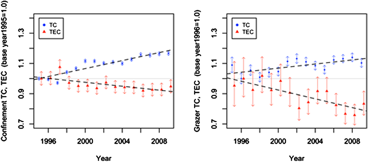
Figure 2. Technical change and technical efficiency change
The positive technical change and increasing efficiency gaps in both systems suggest that some producers have successfully adopted new technologies and improved their management, while others have struggled to keep up with these changes. In particular, the different trends observed for the two systems seem to indicate that a greater share of confinement operations have benefitted from recent technological advances, compared to graziers. This is consistent with a common perception that confinement dairy operations generally follow standardized industry production techniques, while MIG operations involve highly localized and idiosyncratic production practices (mainly due to local soil and microclimate conditions that require experimentation by individual producers).Footnote 17
Declining technical efficiency for both groups means that the productivity gaps among dairy producers are increasing. Dairy producers traditionally have pursued expansions and upgrades in times of high milk prices. However, with the emergence of ever-larger, capital-intensive operations, the standard for efficient operation appears to be raised more frequently and rapidly than before. Those who wait for the next boom to reinvest in their operation are increasingly at risk of being left behind. For graziers, exploring the low-input production system under MIG can risk forgoing an unexpectedly large share of outputs. Rapid reductions in output may in part be a consequence of complying with organic production standards (e.g., about a quarter of the graziers in our sample produced organic milk in all or some of the survey years), which can explain particularly rapid declines in efficiency among graziers. The current analysis ignores the difference in milk quality for the sake of comparability between the two systems.
Turning to the coefficient estimate for the heat index, we find little evidence that warmer summer temperatures negatively affect dairy production of efficient or less-than-efficient producers in Maryland, a result generally consistent with a cross-sectional analysis by Key and Sneeringer (Reference Key and Sneeringer2014). Under multiple climate change scenarios, those authors predict that the annual fluctuation of summer temperatures can on average decrease dairy production across states by 0.60 percent to 1.35 percent by 2030, with varying degrees ranging from less than 0.5 percent in Idaho to about 2.0 percent to 4.5 percent in Texas. Their prediction suggests a very limited impact of about 0.60 percent to 1.00 percent in Pennsylvania, a neighboring state of Maryland.
As for producer characteristics, we find that farm ownership suggests higher efficiency, whereas the impact of having off-farm income is mixed. Higher efficiency for owner-operators in dairy operation is previously reported in Mayen, Balagtas and Alexander (2010). The renter-operator may have lower incentives to invest in on-site production facilities or rent land of lower qualities. In our estimate, having off-farm income is associated with lower efficiency among confinement operations but not among graziers. Theoretical prediction of this effect would be ambiguous, given the complexity of the decision to work off-farm that can be influenced by operator's talents in nonfarming activities as well as his/her tolerance to downside income risks.
In the relevant literature, previous studies find that technical efficiency is associated with operational scale (Kumbhakar, Ghosh, and McGuckin Reference Kumbhakar, Ghosh and McGuckin1991, Tauer and Mishra Reference Tauer and Mishra2006 Byma and Tauer Reference Byma and Tauer2010, Key and Sneeringer Reference Key and Sneeringer2014,); the share of total forage purchases (Mosheim and Lovell, Reference Mosheim and Lovell2009, Cabrera, Solís and del Corral Reference Cabrera, Solís and del Corral2010, Mayen, Balagtas and Alexander Reference Mayen, Balagtas and Alexander2010); the use of total mixed ration (TMR) and daily milking frequency of three times or higher (Cabrera, Solís and del Corral Reference Cabrera, Solís and del Corral2010); producer's education (Stefanou and Saxena Reference Stefanou and Saxena1988, Kumbhakar Reference Kumbhakar1993, Byma and Tauer Reference Byma and Tauer2010); producer's experience (Stefanou and Saxena Reference Stefanou and Saxena1988 Mosheim and Lovell Reference Mosheim and Lovell2009); managerial ability, measured by producer's subjective value of labor or by lagged net income (Byma and Tauer Reference Byma and Tauer2010); the proportion of irrigated area (Kompas and Che Reference Kompas and Che2006); the use of consulting services (Mukherjee, Bravo-Ureta and De Vries Reference Mukherjee, Bravo-Ureta and De Vries2013); and a share of family-labor in the total-labor input (Cabrera, Solís and del Corral Reference Cabrera, Solís and del Corral2010). Also, the output of efficient producers may increase with the use of recombinant bovine somatotropin (rBST) (Cabrera, Solís and del Corral Reference Cabrera, Solís and del Corral2010; Mukherjee, Bravo-Ureta and De Vries Reference Mukherjee, Bravo-Ureta and De Vries2013) and the presence of off-farm income (Kumbhakar Reference Kumbhakar1993 Mayen, Balagtas and Alexander., Reference Mayen, Balagtas and Alexander2010). Some of these characteristics describe the attributes of typical large-scale confinement operations. To be competitive, dairy producers of smaller scales need to keep pace with rising industry standards set by large dairies and, whenever possible, learn from their efficient peers.
4. Conclusions
Amid the increasing consolidation of U.S. dairy production, MIG has been gaining popularity among small- to medium-scale dairies as a low-input, low-output system. This article investigates the nature of technological progress and the technical efficiency of the producer using data on Maryland dairy farms during 1995–2009, a period in which confinement dairies scaled up their operations across the country. On average, technology progressed at 1.21 percent per year for conventional confinement operators and 0.59 percent per year for MIG dairies. Given the difference in the rate of technical change, increased research and development in MIG is needed if it is to be a viable alternative to the confinement dairy system. Examples include investigations into improved breeds of grazing cows, high-yielding varieties of forage crops, and pasture management specific to local microclimates. Additionally, the declining average efficiency for both dairy systems needs to be addressed, for instance, through extension programs that support technology adoption.
On the technical side, by building on the concept of MPI decomposition in a regression framework, we have developed a novel approach to analysis of productivity changes. The method can be used to study production heterogeneity such as the influence of production environments across geographical regions or the impacts of regulations at various phases of implementation. Investigating the properties of the proposed estimator and extending its concept are left for future research. One particular area to add would be an extension of scale efficiency change to the MPI decomposition, which was not pursued in this article due to the limited range of observed operational scales in our data.
Appendix A. Robustness
Table A.1. Marginal Effect Estimates: Panel-Consistent Standard Errors (PCSE)
Table A.2. Marginal Effect Estimates: Frontiers with Non-cumulative Data Points
Table A.3. Marginal Effect Estimates: No Bias-corrections
Table A.4. Marginal Effect Estimates: DEA under Constant Returns to Scale
Appendix B. Parametric Frontier Estimation
We estimate parametric frontiers that are comparable to the semi-parametric frontier in (2). Consider a time-specific Cobb-Douglas production function with an efficiency component u it and a stochastic component v it ;
 $$\eqalign{& \ln f_t^{SF} \lpar {\bi x}_{it}\semicolon \; {\bi w}_t\rpar = \sum\limits_l \alpha _{tl}\ln x_{l\comma \, it} + \beta ^f\lpar {\bi w}_t\comma \; t\rpar - u_{it} + v_{it} \cr & \quad {\rm with}\; u_{it} = {\bi z}_{it}{\bi \delta} ^u + \beta ^u\lpar {\bi w}_t\comma \; t\rpar + \eta _{it} \ge 0\comma \; }$$
where functions β
f
(
w
t
, t) and β
u
(
w
t
, t) are specified as either time-specific intercepts or the combinations of linear time trends and parametric functions of
w
t
. Once the equation (B.1) is estimated, we predict $\widehat{{TGR}}\lpar {\bi x}_{it}\comma \; y_{it}\semicolon \; t\rpar $
from technological parameters and
$\widehat{{TGR}}\lpar {\bi x}_{it}\comma \; y_{it}\semicolon \; t\rpar $
from technological parameters and $\widehat{{TE}}\lpar {\bi x}_{it}\comma \; y_{it}\semicolon \; t\rpar = exp\lpar E\lsqb\! - u_{it}\vert \widehat{{v_{it} - u_{it}}}\rsqb \rpar $
from the residual distribution and re-parametrize them according to specification (3). The two-stage estimation through (B.1) and (3) accommodates flexible specifications for β
f
(
w
t
, t) and β
u
(
w
t
, t), which helps identify TC and TEC without imposing strong distributional assumptions on the error structure.Footnote
18
$\widehat{{TE}}\lpar {\bi x}_{it}\comma \; y_{it}\semicolon \; t\rpar = exp\lpar E\lsqb\! - u_{it}\vert \widehat{{v_{it} - u_{it}}}\rsqb \rpar $
from the residual distribution and re-parametrize them according to specification (3). The two-stage estimation through (B.1) and (3) accommodates flexible specifications for β
f
(
w
t
, t) and β
u
(
w
t
, t), which helps identify TC and TEC without imposing strong distributional assumptions on the error structure.Footnote
18
We estimate (B.1) using several specifications that differ in assumptions on inefficiency u
it
. Following two common specifications of stochastic frontier analysis (SFA), we estimate the efficiency component model of Battese and Coelli (Reference Battese and Coelli1995) (i.e., $u_{it}{\rm \sim} N^ + \lpar \mu _u\lpar {\bi z}_{it}\comma \; {\bi w}_t\comma \; t\rpar \comma \; \sigma _u^2 \rpar $
), previously adopted by Tauer and Mishra (Reference Tauer and Mishra2006), Kompas and Che (Reference Kompas and Che2006), Nehring et al. (Reference Nehring, Gillespie, Sandretto and Hallahan2009), and Mukherjee, Bravo-Ureta and De Vries (Reference Mukherjee, Bravo-Ureta and De Vries2013), and the heteroskedastic inefficiency model of Hadri (Reference Hadri1999) (i.e., u
it
~ N
+ (0,
$u_{it}{\rm \sim} N^ + \lpar \mu _u\lpar {\bi z}_{it}\comma \; {\bi w}_t\comma \; t\rpar \comma \; \sigma _u^2 \rpar $
), previously adopted by Tauer and Mishra (Reference Tauer and Mishra2006), Kompas and Che (Reference Kompas and Che2006), Nehring et al. (Reference Nehring, Gillespie, Sandretto and Hallahan2009), and Mukherjee, Bravo-Ureta and De Vries (Reference Mukherjee, Bravo-Ureta and De Vries2013), and the heteroskedastic inefficiency model of Hadri (Reference Hadri1999) (i.e., u
it
~ N
+ (0, $\sigma _u^2 \lpar {\bf z}_{it}\comma \; {\bf w}_t\comma \; t\rpar \rpar $
), employed by Byma and Tauer (Reference Byma and Tauer2010), Cabrera, Solís and del Corral (Reference Cabrera, Solís and del Corral2010), Mayen, Balagtas and Alexander (2010), and Key and Sneeringer (Reference Key and Sneeringer2014).Footnote
19
Both cases assume that the residual components u
it
and v
it
are uncorrelated with
$\sigma _u^2 \lpar {\bf z}_{it}\comma \; {\bf w}_t\comma \; t\rpar \rpar $
), employed by Byma and Tauer (Reference Byma and Tauer2010), Cabrera, Solís and del Corral (Reference Cabrera, Solís and del Corral2010), Mayen, Balagtas and Alexander (2010), and Key and Sneeringer (Reference Key and Sneeringer2014).Footnote
19
Both cases assume that the residual components u
it
and v
it
are uncorrelated with $f_t^{SF} \lpar .\rpar $
and with one another. Additionally, we estimate an OLS specification with producer-specific fixed effects, say
$f_t^{SF} \lpar .\rpar $
and with one another. Additionally, we estimate an OLS specification with producer-specific fixed effects, say $\beta _i^u \lpar {\bf w}_t\comma \; t\rpar $
, and back out parameters of the frontier and efficiency relative to the smallest producer effect (e.g., Schmidt and Sickles, Reference Schmidt and Sickles1984; Cornwell, Schmidt and Sickles, Reference Cornwell, Schmidt and Sickles1990). The OLS specification does not invoke distributional assumptions of SFA but is influenced on the precision of estimated producer effects.
$\beta _i^u \lpar {\bf w}_t\comma \; t\rpar $
, and back out parameters of the frontier and efficiency relative to the smallest producer effect (e.g., Schmidt and Sickles, Reference Schmidt and Sickles1984; Cornwell, Schmidt and Sickles, Reference Cornwell, Schmidt and Sickles1990). The OLS specification does not invoke distributional assumptions of SFA but is influenced on the precision of estimated producer effects.
In Table B.1, we selectively report some results for confinement operations among our estimates of equation (B.1) under a range of conceivable specifications. The estimation for graziers was mostly unsuccessful (i.e., failing to converge under SFA). The three specifications (SFA-1, SFA-2, and OLS-1) in the table differ in their parameterizations of inputs (i.e., acreage variables omitted under SFA-1 and SFA-2), time trends (i.e., a linear trend under SFA-1 and time-specific fixed effects under SFA-2 and OLS-1), and efficiency (i.e., mean-shifted efficiency under SFA-1, heteroskedastic efficiency under SFA-2, and producer fixed effects under OLS-1). Two out of three specifications (SFA-1 and OLS-1) result in qualitatively similar estimates of TC and TEC to those obtained under the nonparametric model.
In the current study, many parametric specifications fail to converge or are unable to yield sensible results likely due to the mismatch between the assumptions of SFA and the nature of heterogeneity in our data. Note that this is not an issue of small sample size but is a general limitation of the parametric frontier approach that relies on a presumed shape of the efficiency distribution. The high importance of relative inefficiency to stochastic noise, as well as the large heterogeneity in observed decisions, tends to exacerbate the problem, which may explain particularly unsuccessful estimation for graziers (unreported).
Table B.1. Stochastic Frontier Estimates (Confinement)


 Open access