


Pathways of movement physically map social networks of communication, interaction, and organization (Erikson Reference Erickson, Snead, Erickson and Darling2009; Snead Reference Snead, Alcock, Bodel and Talbert2012; Snead et al. Reference Snead, Erickson, Andrew Darling, Snead, Erickson and Darling2009). For example, the Roman Empire used a complexly integrated system of paved roads and bridges to resituate provincial societies into a broader economic and cosmopolitan world and to accelerate connectivity across the Mediterranean (Hitchner Reference Hitchner, Alcock, Bodel and Talbert2012). In the Bolivian Amazon, people built raised earthen causeways with associated canals to improve, channel, and control the circulation of water and people across a large, formalized landscape (Erikson and Walker Reference Erickson, Walker, Snead, Erickson and Darling2009). In these instances, and many others, the study of where pathways go and how they were built has helped archaeologists understand systems of social exchange and interaction.
The use of lidar in archaeological research has significantly expanded archaeologists’ ability to detect, visualize, and map certain pathways, such as roads (Azizi et al. Reference Azizi, Najafi and Sadeghian2014; Buján et al. Reference Buján, Guerra-Hernández, González-Ferreiro and Miranda2021; Chase et al. Reference Chase, Chase, Chase, Masini and Soldovieri2017; Ferraz et al. Reference Ferraz, Mallet and Chehata2016; Friedman et al. Reference Friedman, Sofaer and Weiner2017). Although there has been considerable development in using lidar to detect and map roads, less attention has been given to studying road morphology using lidar. Here, a method that visualizes and statistically compares road profiles using elevation values extracted from lidar-derived digital elevation models (DEM) is presented. This method is demonstrated using a case study of Chaco Roads from the US Southwest.
LIDAR FROM THE PROFILE VIEW
Most archaeologists who study roads using lidar have focused on locating and mapping road segments in raster-based lidar products, resulting in a suite of techniques that make it easier to identify ephemeral, overgrown, and previously unidentified roads (Chase et al. Reference Chase, Chase, Awe, Weishampel, Iannone, Moyes, Yaeger and Kathryn Brown2014, Reference Chase, Chase, Chase, Masini and Soldovieri2017; Cifani et al. Reference Cifani, Opitz and Stoddar2015; Gasparini et al. Reference Gasparini, Moreno-Escribano and Monterroso-Checa2019; Johnson and Ouimet Reference Johnson and Ouimet2014; Štular et al. Reference Štular, Kokalj, Oštir and Nuninger2012). In addition to visualization techniques, numerous methods for detecting roads in lidar data using computer automation have been developed (Azizi et al. Reference Azizi, Najafi and Sadeghian2014; Buján et al. Reference Buján, Guerra-Hernández, González-Ferreiro and Miranda2021; Chen et al. Reference Chen, Zhang and Tao2019; Ferraz et al. Reference Ferraz, Mallet and Chehata2016; Mayoral et al. Reference Mayoral, Toumazet, Simon, Vautier and Peiry2017; White et al. Reference White, Dietterick, Mastin and Stronhman2010), often with impressive outcomes—such as the ability to detect and classify roads in lidar data with over 90% accuracy and confidence (e.g., Buján et al. Reference Buján, Guerra-Hernández, González-Ferreiro and Miranda2021). Although visualization and detection methods deserve continued attention, they have a limited use for studying road morphology because they primarily give the researcher an aerial perspective of the feature. For example, one of the most useful techniques for visualizing roads in lidar data is through methods that amplify topographic relief, such as a hill-shade technique or sky-view factor (Devereux et al. Reference Devereux, Amable and Crow2008; Kokalj et al. Reference Kokalj, Zakšek, Oštir, Opitz and Cowley2013), which intensifies the road's signature from the aerial view. Yet, only a few characteristics—such as length, linearity, and width—can be identified from this view, and other diagnostic features, such as depth and the extent of construction, require a profile view. For example, longitudinal profiles (a cross section along the linear axis of a road) can show if and how the road grade was modified in relationship to nearby terrain, and transverse profiles (a cross section oriented perpendicular to the road) can reveal the depth, shape, and character of the roadbed (Nials Reference Nials and Kincaid1983).
Several studies have used lidar to produce high-resolution transverse road profiles (Friedman et al. Reference Friedman, Sofaer and Weiner2017; Romain and Burks Reference Romain and Burks2008), allowing the researchers to identify morphological characteristics and construction techniques, such as the presence of bounding earthen embankments. Yet, these studies produced a small number of road profiles as opposed to a comprehensive array of profiles across entire features. Furthermore, although many built-in GIS profile tools allow a researcher to visualize road profiles using lidar data, they are not suited for comparing profile characteristics. Therefore, existing methods are not sufficient for either the systematic production or statistical comparison of road profiles using lidar data.
Therefore, to expand the toolkit that archaeologists can use to study road profiles using lidar, an automated method for developing and comparing profiles is presented here for use in any context where road locations are known and have been documented remotely. The method is developed in R (a statistical and geospatial software package) and illustrated through a case study on Chaco roads found in the US Southwest, where roads played an important role in indigenous mobility and landscape making (Darling Reference Darling, Snead, Erickson and Darling2009; Ferguson et al. Reference Ferguson, Lennis Berlin, Kuwanwisiwma, Snead, Erickson and Darling2009; Snead Reference Snead, Snead, Erickson and Darling2009). To contextualize the Chaco case study, a brief synthesis of Chaco roads is presented and then a step-by-step procedure for implementing the profile method is detailed, followed by results from the case study.
CHACO ROADS
During the ninth through the mid-twelfth centuries AD, Chaco Canyon, located in present-day New Mexico, became the center of extensive ceremonial, political, economic, and social networks that are evidenced by a wide array of material culture, including roads. Chaco roads are linear, earthen depressions that are often at least 10 m wide; straight (rather than terrain following); and associated with Chaco-era communities (Figure 1). Certain Chaco roads, such as the North Road and South Road, are frequently referred to as regional features because they are particularly wide, continuous features that physically connect Chaco communities located far outside of the canyon with communities inside the canyon. Other roads likely served local purposes, given that they extend only a short distance away from a community and do not articulate with any other roads (Stein Reference Stein and Kincaid1983). Local and regional Chaco roads were probably used for many reasons—from pilgrimage routes (Judge Reference Judge, Cordell and Gumerman1989; Van Dyke Reference Van Dyke2007) to long-range transportation paths (Betancourt et al. Reference Betancourt, Dean and Hull1986; Field et al. Reference Field, Heitman and Richards-Rissetto2019) and as symbolic connections with important geographic features, directions, and/or noncontemporaneous sites (Fowler and Stein Reference Fowler, Stein and Doyel1992; Kantner Reference Kantner1997; Kincaid Reference Kincaid1983; Lekson Reference Lekson2015; Mills Reference Mills2002; Roney Reference Roney and Doyel1992; Sofaer et al. Reference Sofaer, Marshall, Sinclair and Aveni1989; Vivian Reference Vivian1997).
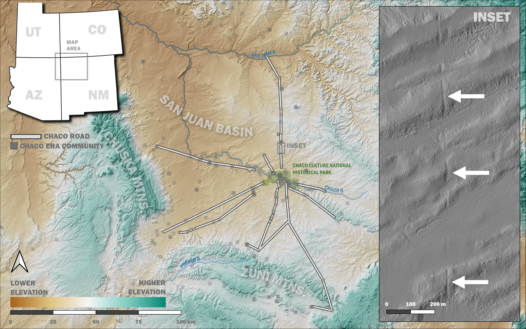
Figure 1. Location of major or well-studied Chaco roads within the San Juan Basin. Inset shows section of the North Road in a hill-shaded relief of the lidar-derived DEM.
In-depth research on Chaco roads began in the 1960s, when researchers began using aerial photography to identify and document Chaco roads (Kincaid Reference Kincaid1983; Lyons and Hitchcock Reference Lyons, Hitchcock, Lyons and Hitchcock1977; Morrison Reference Morrison1973; Nials et al. Reference Nials, Stein and Roney1987; Obenauf Reference Obenauf1980), culminating with the Chaco Roads Project (CRP), which studied Chaco roads via aerial imaging, survey, and excavation. The CRP found that some Chaco roads were engineered and constructed, often through excavation to a compact substrate and the removal of materials from the road surface, and roads were also episodically maintained or cleaned (Nials Reference Nials and Kincaid1983:6-24, 6-31, 6-45). Although the CRP also demonstrated that many Chaco roads had generally uniform characteristics, they noted that the ceramic and architectural traits associated with roads—such as cairns, walls, and stone circles—could vary considerably (Kincaid Reference Kincaid1983, Nials et al. Reference Nials, Stein and Roney1987). Perhaps most importantly, the CRP (and subsequent work from Friedman et al. Reference Friedman, Sofaer and Weiner2017; Hurst and Till Reference Hurst, Till and Cameron2009; Till Reference Till2001, Reference Till2017; Vivian Reference Vivian1997) has highlighted the need to study Chaco roads through multiple methods, including ground survey and aerial imaging.
However, a complete study of all Chaco roads through mixed methods seems unlikely to be achieved. There are at least several hundred kilometers of Chaco roads, of which only a small number have been studied on the ground (Kincaid et al. Reference Kincaid, Stein, Levine and Kincaid1983). Furthermore, many roads are degrading as a result of modern land practices (Friedman et al. Reference Friedman, Sofaer and Weiner2017; Heitman and Field Reference Heitman, Field, Van Dyke and Heitman2021). Consequently, rapid, effective methods for studying Chaco roads from both ground- and aerial-based perspectives are needed. Friedman and colleagues (Reference Friedman, Sofaer and Weiner2017) have demonstrated that lidar is a useful method for this task by producing high-resolution visualizations and transverse profiles of several Chaco roads. Their methods are expanded upon here, where transverse profiles are produced for nearly 45 km of Chaco roads using lidar-derived elevation data.Footnote 1
THE METHOD
The method presented here uses an R-scriptFootnote 2 to systematically produce transverse transects across road locations, extract and normalize elevation data using these transects, and create road profiles from the elevation data. Transects are then statistically compared to understand the degree of uniformity in road profile shape among and between features. Each step in this method is discussed and illustrated using the Chaco roads case study. The accompanying code for each step can be found in the repository (https://github.com/sfield2/Lidar-derived-profiles). Before any analysis can take place, however, a geodatabase of road locations (some of which have already been ground truthed) is required. The geodatabase of Chaco road locations was developed from analog maps and photographs of Chaco roads (Kincaid Reference Kincaid1983; Nials et al. Reference Nials, Stein and Roney1987; Obenauf Reference Obenauf1980), as well as a hill-shaded version of the DEM produced by the Sanborn Map Company. Roads in the geodatabase include segments that visually resemble a Chaco road from the plan view and have been mapped or verified by previous researchers (Friedman et al. Reference Friedman, Sofaer and Weiner2017; Kincaid Reference Kincaid1983; Nials et al. Reference Nials, Stein and Roney1987; Obenauf Reference Obenauf1980), as well as segments that resemble a Chaco road from the plan view and are in line with other previously mapped segments but have not been specifically mapped or verified by previous researchers. The sample of Chaco roads studied here include segments of the North Road, South Road, Southeast Road, Mexican Springs Road, Casa del Rio to Lake Valley Road (a possible portion of the hypothesized West Road), Ah-Shi-Sle-Pah Road (also referred to as the Peñasco Blanco to Ah-Shi-Sle-Pah Road), Pueblo Pintado Road, Chacra Face Road, a cluster of roads near Pueblo Alto, and a road just south of Peñasco Blanco (Table 1; Figure 2). Not all Chaco roads, such as the Coyote Canyon Road, were sampled for this study because visible segments were not identified in the Sanborn lidar survey data.
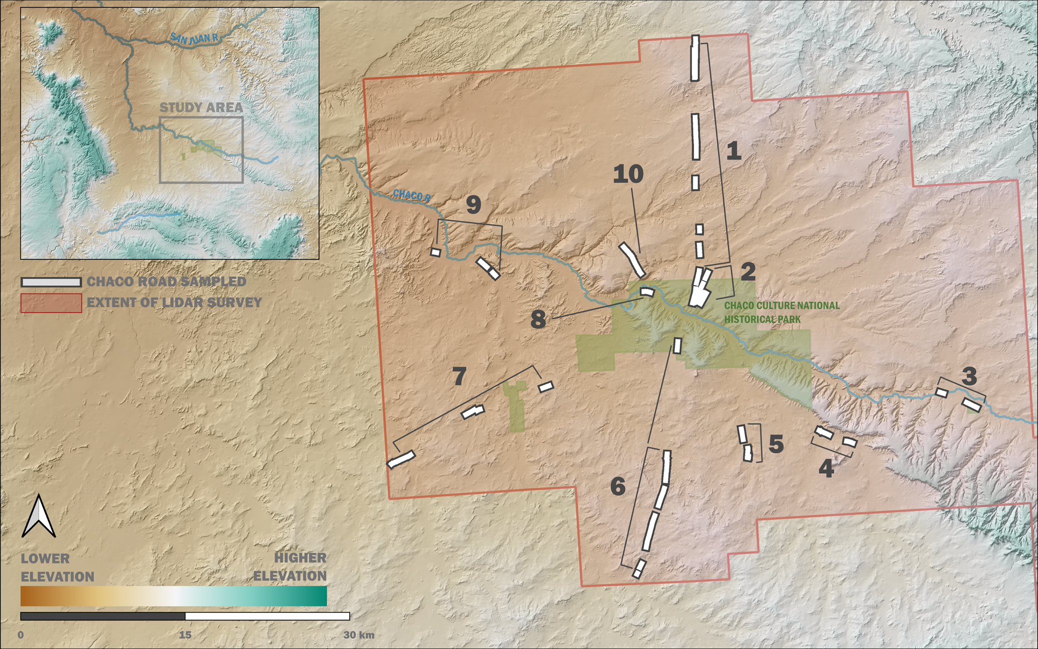
Figure 2. Location of Chaco roads that were sampled for this study: (1) North Road, (2) Pueblo Alto Roads, (3) Pueblo Pintado Road, (4) Chacra Face Road, (5) Southeast Road, (6) South Road, (7) Mexican Springs Road, (8) Peñasco Blanco Road, (9) Casa del Rio to Lake Valley Road, (10) Ah-Shi-Sle-Pah Road. Extent of Sanborn lidar survey marked in red.
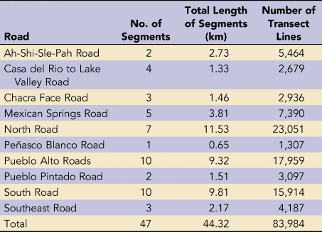
Table 1. Segments of the Chaco Road Network Captured in the Lidar Survey.
Step 1: Create Transverse Transects across Length of All Roads
Road shapefiles were imported into R, and digital transverse transects were created as discrete shapefile lines at half-meter intervals along every road. Transverse transects were created at a length of 50 m and at half-meter intervals to ensure that raster cells representing the full road and its adjacent landscape would be captured (Kincaid Reference Kincaid1983). If transects had been produced at 1 m or greater intervals, then some of the 1 m resolution DEM raster cells may not have been extracted and visualized due to inconsistencies in the DEM resolution and transect spacing. For example, east–west transect lines that are spaced at 1.5 m intervals would not capture every cell of the 1 m raster that is aligned north–south, and therefore portions of the road profile would not be visualized. In total, 83,984 transverse transect lines were created for this case study (Table 1).
Step 2: Extract and Normalize Elevation Data
For each DEM raster cell crosscut by a transect, two data points were recorded. The first data point is the elevation value (in meters), which is extracted from the lidar-derived DEM. The second data point is the point of measure of the corresponding raster cell (i.e., the second through nth order of each cell crosscut by the transect in respect to the first crosscut cell). The elevation values extracted and the number of cells crosscut during this process varied greatly due to significant topographic variation in the study area, and because of differences in the directional relationship between the transect lines and DEM raster grid. For example, a 50 m long east–west transect line is directly perpendicular to the north–south-arranged raster grid, resulting in 50 elevation values and 50 points of measure being recorded. Alternatively, an equal length transect oriented NE-SW can crosscut more than 50 raster cells, because the transect line is not perpendicular to the raster grid. As a result, the number of values extracted by transects in this study range from 50 to 73 values.
If the extracted data were plotted with the point of measure along the x-axis and the elevation value along the y-axis, profiles could not be graphically compared due to dissimilar elevation ranges and lengths. To normalize the elevation values in the dataset, the second through nth number of extracted values in each transect were calculated as a positive or negative change from the first extracted value. For example, the value of the first raster cell that is intersected by “Transect #1” is 1,946.21 m, and the second and third values are 1,946.41 and 1,946.31 m, respectively. After normalizing, the first, second, and third values from “Transect #1” are 0, −0.02, and −0.01 m, respectively. To normalize transect lengths, the formula A*(B/C) was applied to all points of measure, where A is the original point of measure recorded, B is the length of the transect, and C is number of cells crosscut by each transect. For example, if a 50 m long transect results in 60 cells being crosscut (i.e., 60 points of measure), the normalized first, second, and third points of measure would be 0.83, 1.67, and 2.5; the last three values would be 48.3, 49.17, and 50.
Consequently, following normalization, any transect can be directly compared to any other transect in the dataset. For example, profiles can be plotted with the normalized depth along the x-axis and the normalized point of measure along the y-axis to see the shape of any single section of road (Figure 3). Furthermore, data from a single transect can be smoothed with a local regression model to better understand the shape of the profile, or multiple smoothed or unsmoothed profiles can be plotted to understand how the road profile changes along the length of the road (Figure 3). Additionally, all values from the same road can be plotted to understand the complete surface of the road and its adjacent landscape (Figure 4).
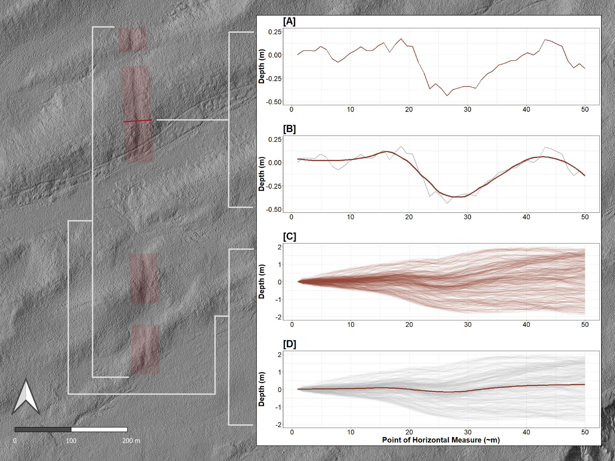
Figure 3. Example of the sampling process from the North Road: (a) the normalized values from a single transect plotted in red; (b) the normalized values from a single transect plotted in gray, and a local regression of the values from a single transect plotted in red; (c) the normalized values from multiple transects plotted in red; (d) the normalized values from multiple transects plotted in gray, and a local regression of all values from multiple transects plotted in red.
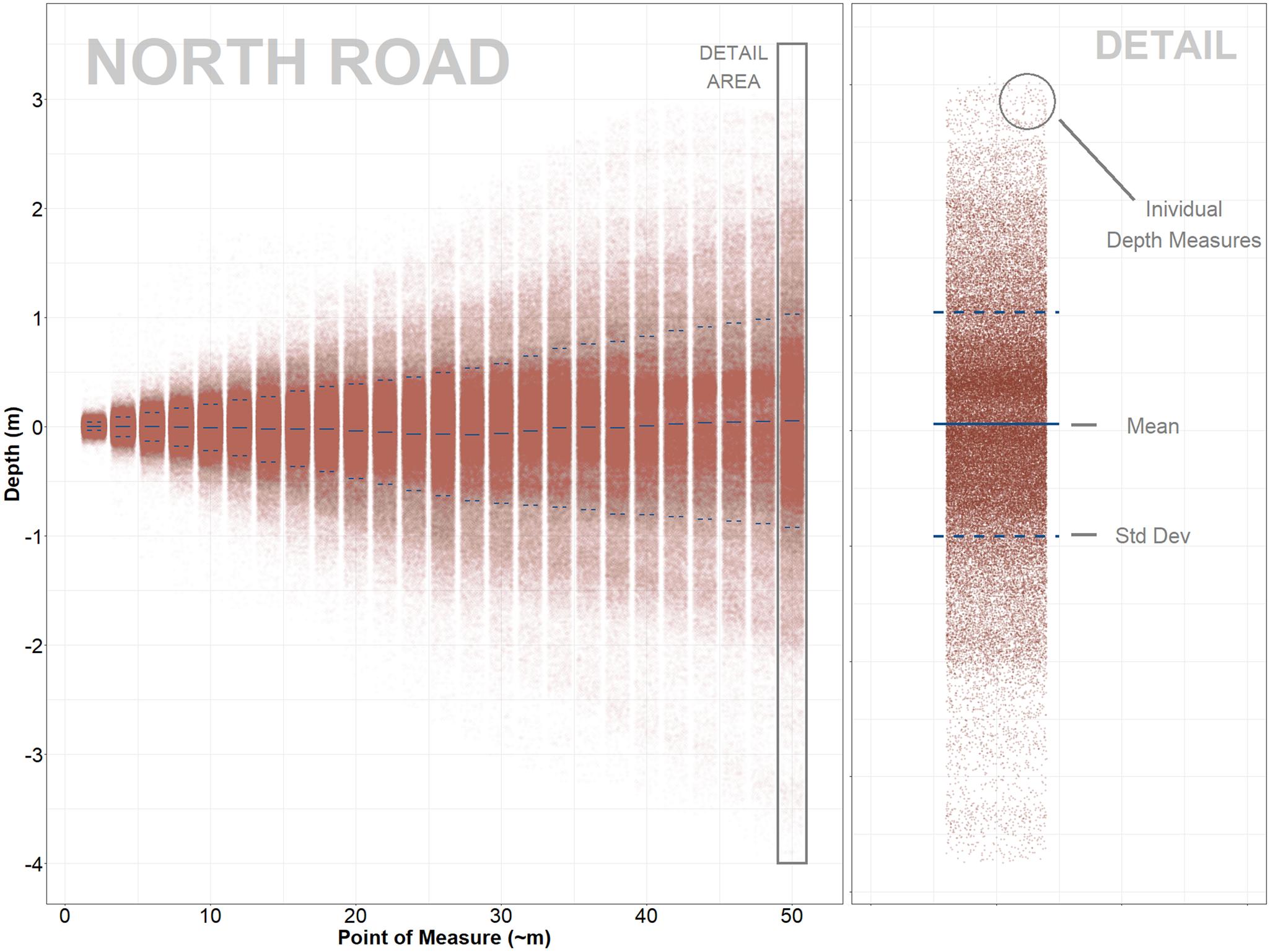
Figure 4. Plot of all extracted values for the North Road. Each red dot represents one extracted value. The mean of all values is plotted as a solid blue line. The standard deviation of all values is plotted as a dotted blue line.
Step 3: Determine Common Morphology
An inherent limit of remote sensing is the inability to verify if features are archaeological, which often requires ground truthing via survey or excavation. Therefore, it is important to develop profiles from previously ground-truthed road sections and to critically examine what these features look like from the profile view. In the Chaco landscape, the two roads that have been studied most thoroughly are the North Road and South Road, which are two regional roads that emanate northward and southwestward from Chaco Canyon. Both features are well defined, are particularly wide, and have been studied thoroughly via aerial photography, lidar, ground survey, and minor excavations (Friedman et al. Reference Friedman, Sofaer and Weiner2017; Kincaid Reference Kincaid1983; Nelson and McAnany Reference Nelson and McAnany1982; Nials et al. Reference Nials, Stein and Roney1987; Obenauf Reference Obenauf1980). Therefore, these features are some of the best candidates for establishing what ground-truthed Chaco roads look like from the profile view. Plotting all transects of the North and South Road show a messy, poorly defined array of profiles, making it difficult to determine any definitive characteristics of each road (Figure 5).
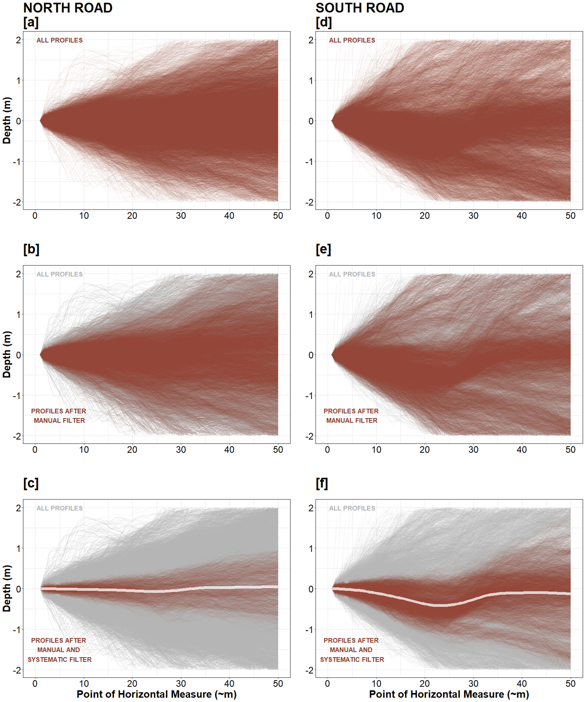
Figure 5. Demonstration of the filtering process for the North and South Roads: (a, d) all profiles for each road; (b, e) all profiles for each road following manual filter; (c, f) all profiles for each road following manual and systematic filter, and a local regression model of all remaining profiles plotted as a white line.
Therefore, transects of the North Road and South Road were manually filtered to remove transects that represented the least visible road segments and systematically filtered to remove profiles with the least common morphology. Specifically, the systematic filter removes all transects containing a depth value greater than one standard deviation away from each road's mean depth at every tenth point of measure (i.e., the tenth, twentieth, thirtieth, and so-on elevation value that was extracted along each transect [Figure 5]). Once filtered, a local regression model was calculated from all profiles remaining to show the form of the most common, diagnostic portions of the North and South Road. An average of the two regression lines was taken to produce a composite profile representing the typical form of a well-defined, ground-truthed Chaco road (Figure 6).
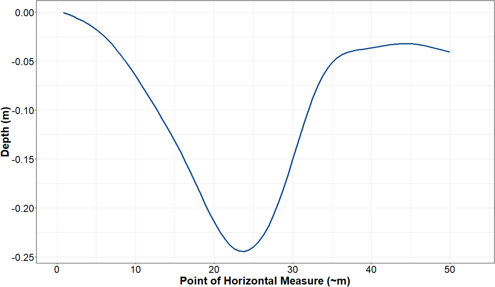
Figure 6. Composite profile, derived from the North and South Roads and representing the typical form of a well-defined, ground-truthed Chaco road.
The composite profile shows a parabolic, symmetrical depression that is approximately 20 m wide, 25 cm deep, and bounded on at least one side by a slight berm, and it is set within a relatively flat landscape. The shape of the composite profile is deeper than at least one other lidar-derived profile of the North Road (depth of 9.1 cm) produced by Friedman and colleagues (Reference Friedman, Sofaer and Weiner2017). This difference is likely due to the incorporation of the South Road in this analysis, which is characterized by a deeper profile than that of the North Road. The composite profile is also at the upper limits of prior estimates regarding the width of Chaco roads (Hurst and Till Reference Hurst, Till and Cameron2009; Nials Reference Nials and Kincaid1983; Stein Reference Stein and Kincaid1983; Till Reference Till2001, Reference Till2017; Vivian Reference Vivian1997).
Step 4: Testing Similarity with the Composite
The amount of similarity between the composite profile and all other profiles was iteratively tested to understand how many transects closely resemble the form of the composite. Similarity was tested using an approach that samples a single transect, produces a smoothed profile of the sample data using a local regression model, calculates the slope of the regression line, and compares it to the slope of the composite profile using a two-tailed Kolmogorov-Smirnov (K-S) test (Figure 7). To focus the comparison on the road surface itself, the slope of the smoothed sample profile and the slope of the composite profile were limited by clipping the borders of each profile before the K-S test was conducted. The K-S test produces a D-statistic, which represents the amount of difference between the sample and composite profile, as well as a p-value. A strong match between a sample profile and the composite profile is defined as any test resulting in a p-value less than 0.05 and a D-statistic lower than the critical value of 0.416, where α = 0.001 and n1 and n2 = 44 (i.e., the number of points that comprise the profiles being compared). Strong matches represent sample profiles that strongly resemble the composite profile.
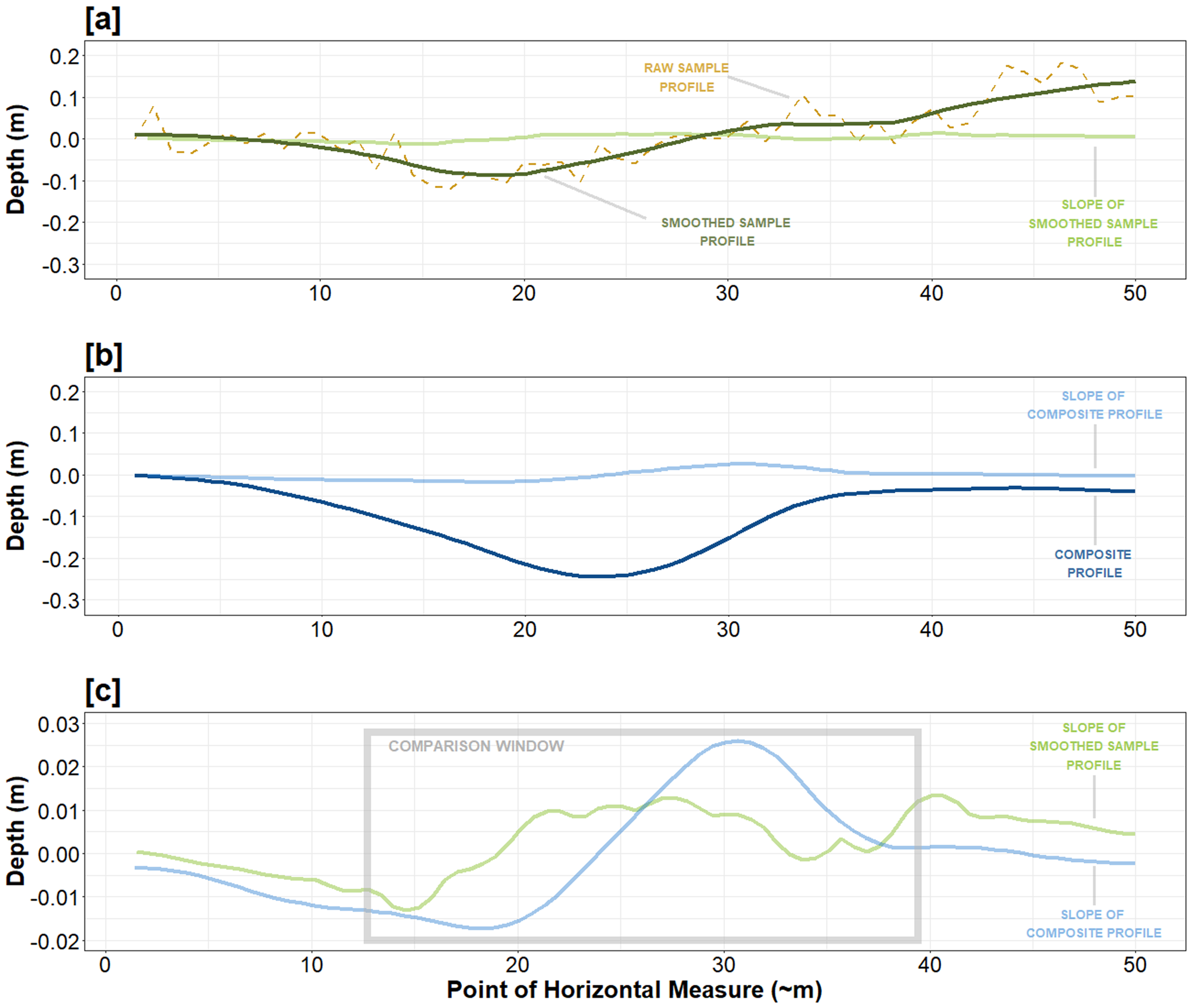
Figure 7. Example of the K-S test process: (a) sample profile, (b) composite profile, (c) comparison of the sample profile slope and composite profile slope. The sample transect exemplified is a strong match to the composite.
Even among roads that are very similar to the composite, not all sections can be expected to match strongly due to the effects of erosion and land use (Friedman et al. Reference Friedman, Sofaer and Weiner2017; Heitman and Field Reference Heitman, Field, Van Dyke and Heitman2021; Kincaid et al. Reference Kincaid, Stein, Levine and Kincaid1983), as well as the general variability of roads that are built over long distances. Therefore, to determine how often ground-truthed roads should be expected to match the composite, the K-S test was first conducted for all profiles of the North and South Roads. This analysis showed that nearly 30% of all transects in the North Road strongly match the composite and that approximately 22% of all transects in the South Road strongly match the composite (Table 2). Based on these results, it is suggested that any road with at least 22% of strongly matching profiles is likely similar in overall form to the North and South Roads. Additionally, results from the K-S test can be merged back with the transect shapefiles, allowing researchers to conduct spatial analyses, such as measuring if strongly matching profiles are closer to residential sites, or if non-matching profiles are located in landscapes with more profound erosional processes (Figure 8).
Table 2. Results of the K-S Test.
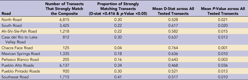
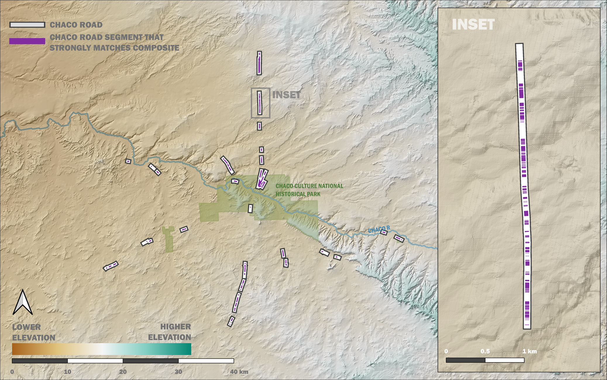
Figure 8. Location of Chaco road profiles that strongly match the composite.
INTERPRETING CHACO ROAD PROFILES
Among the Chaco roads sampled here, five contain more than 22% of profiles that strongly match the composite: the Pueblo Pintado Road, Pueblo Alto Roads, Southeast Road, Casa del Rio to Lake Valley Road, and Ah-Shi-Sle-Pah Road. Two other roads contain somewhat less than 22% of strongly matching profiles—the Mexican Springs Road and the Peñasco Blanco Road—and only the Chacra Face Road is characterized by a notably low proportion of strongly matching profiles (Table 2). These results confirm prior suggestions that the Chacra Face Road is likely not a Chaco Road (Nials et al. Reference Nials, Stein and Roney1987; Roney Reference Roney and Doyel1992; Snead Reference Snead2017; Vivian Reference Vivian1997). These results also indicate that the Ah-Shi-Sle-Pah Road is morphologically consistent with features similar to those of the North Road and South Road, despite it being interpreted as a local feature (rather than a regional feature) because it neither articulates with larger roads nor terminates at a Chaco-era community (Stein Reference Stein and Kincaid1983). Furthermore, the K-S tests underscores that the North Road, South Road, Pueblo Pintado Road, and Pueblo Alto Roads are some of the most characteristic Chaco roads, containing well-defined features, long stretches of visible depressions, and berming (Nials Reference Nials and Kincaid1983).
However, the degree of (dis)similarity between sampled roads and the composite is not fully represented by the K-S test. Plotting strongly matching profiles (Figure 9) shows that some roads with a high proportion of strongly matching profiles are not as visually similar to the North and South Roads. For instance, the K-S test indicates that 41% of profiles from the Southeast Road strongly match the composite, suggesting a strong resemblance between the Southeast Road and the typical form of a ground-truthed Chaco road—a surprising result given that the Southeast Road has been previously discounted as a Chaco Road (Kantner Reference Kantner1997; Nials et al. Reference Nials, Stein and Roney1987; Vivian Reference Vivian1997). Yet, although the strongly matching profiles of the Southeast Road have the same general shape as the composite, they represent a road surface that is more shallow, more ephemeral, and thinner than the North and South Roads (Figure 9). Therefore, in this instance, the K-S test seems to overestimate the similarity between the Southeast Road and the expected form of ground-truthed Chaco roads, thereby cautioning the need to cross-reference K-S results with qualitative comparisons. Similarly, 30% of profiles from the Casa del Rio to Lake Valley Road strongly match the composite, although large sections of the road are much steeper than the North and the South Road and consequently do not match the composite (Figure 9). Therefore, only certain segments of the Casa del Rio to Lake Valley Road (as opposed to the entire feature) can be considered a strong match, suggesting that non-matching sections have been significantly more eroded over time—or perhaps were differently built, used, or maintained by people during the Chaco era.
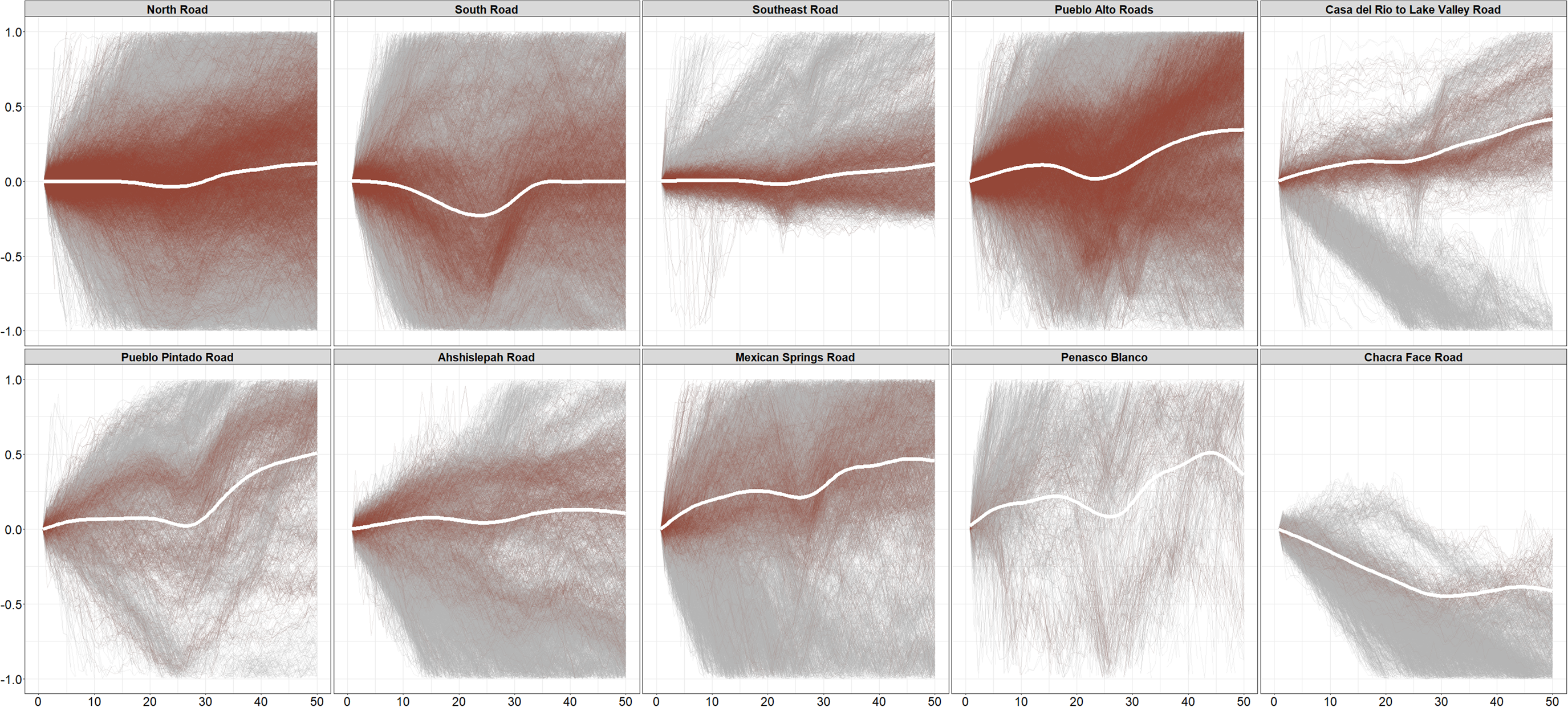
Figure 9. All profiles examined in this study are plotted as solid gray lines. All profiles considered a strong match to the composite are plotted as solid red lines. Ordered by strength of match to the North and South Roads.
Differences between the K-S test and the plotted results can also be seen in the Mexican Springs Road and the Peñasco Blanco Road. Both features contain less than 22% of profiles that strongly match the composite. However, the profile characteristics of both roads show many of the same characteristics of the composite, such as berming on one or both sides and a road surface that is symmetrical and approximately 25 cm deep (Figure 9). The contradiction between the roads’ appearance and the K-S results may be due to different building practices between the Mexican Springs and Peñasco Blanco Roads and the North and South Roads. When examining the Peñasco Blanco Road, the CRP verified the feature and noted that it was built as a raised road, with both sides of the roadbed projecting above surrounding terrain (Nials Reference Nials and Kincaid1983:6–11). This form is apparent in the profiles developed here (Figure 9), not only for the Peñasco Blanco Road but also for the Mexican Springs Road. This result suggests that the Mexican Springs Road was also built as a raised roadbed and, perhaps, that both roads represent a slightly different class of Chaco road that was elevated rather than excavated. This is a particularly important finding for the Mexican Springs Road, which has previously been debated as a Chaco road (Kantner Reference Kantner1997; Nials et al. Reference Nials, Stein and Roney1987; Vivian Reference Vivian1997).
It will take additional research to determine if the strong similarity between certain roads and the composite are an indication that these features were built, used, and maintained by past people in the same way or because they have since eroded similarly. There is some evidence that erosional processes have influenced the uniform appearance of Chaco roads. For example, tentative results presented by Clark and Fristchle (Reference Clark and Fritschle2011) suggest that erosional and natural factors can help predict visible and non-visible Chaco roads. Additionally, Nials (Reference Nials and Kincaid1983) suggests that a symmetrical profile depression, which is common in Chaco road profiles, indicates some degree of uniform erosion along the road surface. Yet, it seems unlikely that erosion explains all of the uniformity in Chaco road profiles, given that strongly matching profiles identified here are found all across the Chaco landscape (Figure 8), where erosional processes—such as water, wind, and different soils—varied. Furthermore, a suite of common but nonuniversal attributes and forms are also characteristic of other types of Chaco architecture. For example, although Chaco great house architecture is frequently characterized by oversized rooms and enclosed kivas, these features are not present at all great houses (Van Dyke Reference Van Dyke1999, Reference Van Dyke2003), and Chaco house architecture is more broadly characterized by a continuous range in the presence and expression of specific features (Heitman Reference Heitman2011; Throgmorton Reference Throgmorton, Halperin and Schwartz2016; Van Dyke Reference Van Dyke2003). Therefore, it seems likely that at least some of the commonality between road profiles demonstrated here is a result of “a prevailing concept of what constituted a Chacon road and its context” (Vivian Reference Vivian1997:29) that was practiced by past people living in the Chaco landscape.
CONCLUSION
The method presented here offers a systematic means of producing and comparing road profiles using lidar-derived elevation data. Through this method, individual road profiles or entire surfaces can be visualized, filtered, and examined. Ground-truthed roads can also be analyzed to determine the most common, diagnostic form of a specific type of road and used to understand how frequently other roads resemble that form. In the case study on Chaco roads, this method has enabled the analysis of 10 different roads, establishing a threshold of what the most definitive Chaco roads look like from the profile view and determining how frequent this form is across the Chaco landscape. The morphological uniformity observed across certain Chaco roads reiterates that some roads were built in similar ways, and therefore that Chaco roads were one aspect of an intentionally constructed landscape that was purposefully imbued with cultural, religious, and political meaning. This case study has also underscored the common attributes that characterize prominent Chaco roads—such as the North, South, Pueblo Alto, and Pueblo Pintado Roads—and suggested that certain roads thought to be non-archaeological, such as the Mexican Springs and Southeast Road, deserve continued attention before being disqualified as Chacoan features.
Beyond the findings relevant to the archaeology of Chaco, this method is an addition to the growing suite of tools used for documenting and comparing landscapes using remotely sensed data. Although this method demonstrates the utility of studying lidar from a profile view, it is not a replacement for ground truthing, which will remain critical for studying ephemeral features such as roads, particularly in the Chaco landscape. However, if ground truthing cannot be pursued due to land access or degradation, this method can be used to leverage previous ground truthing and create a more informed analysis of remotely sensed data.
Acknowledgments
I would like to thank Donna Glowacki, Carrie Heitman, Mark Schurr, Ian Kuijt, Alan Hamlet, and Kelsey Reese for their thoughtful discussion about the ideas presented here. I would also like to thank Paul Reed and Tim Hovezak for their invaluable contribution and permission toward the procurement and access of data used in this research. Finally, I would like to the express my gratitude to the member of the Chaco Roads Research Project, Margaret Obenauf, Jonathan Till, Winston Hurst, and countless others whose foundational and continued work has been an invaluable service to Chaco road research and a personal use to my own ideas on Chaco roads.
Funding Statement
This research received no specific grant from any funding agency in the public, commercial, or not-for-profit sectors.
Data Availability Statement
The lidar data used in the analysis of Chaco roads located in the San Juan Basin was collected in 2016 through a Bureau of Land Management survey contracted to the Sanborn Map Company. The author received permission to use the data through Archaeology Southwest, following joint analysis of the data for a 2019 report on the protection of the Greater Chaco Landscape. The data used and analyzed by the author and Archaeology Southwest is stored offline. However, equal resolution lidar data is now available for much of the study area and can be accessed through the United States Geological Survey (USGS [https://apps.nationalmap.gov/downloader/#/]). All scripts used to analyze the data are available at https://github.com/sfield2/Lidar-derived-profiles.
Competing Interests
The author declares none.
Supplemental Material
For supplemental material accompanying this article, visit https://github.com/sfield2/Lidar-derived-profiles.


 Open access