


7.1 Physical Weathering and Soil Mineral Matter
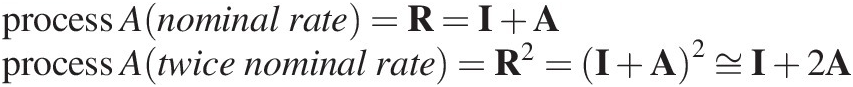
The previous chapter discussed models for soil depth alone and didn’t provide any information about how the soil varied within the profile. In this chapter we talk about models for predicting the particle size grading down the soil profile.
In this chapter we discuss processes that change the soil particles physically with an emphasis on the particle size distribution. Chemical transformations will be discussed in Chapter 8. We will not discuss the evolution of the strength of the rock/soil fragments, though this may be important in some circumstances when overburden load is high (e.g. deep inside mine spoil waste dumps).
The focus here is on fragmentation processes where larger rock and soil particles physically break down into smaller particles and where the fragmentation process itself does not change the chemistry of the particles. However, we make no presumption about the processes that cause fragmentation. Fragmentation may be caused by physical, chemical or biological processes, including the following:
Physical: cycles of salt crystallisation in cracks may wedge open existing cracks or pits, as may cycles of freeze-thaw. Rapid heating and cooling (e.g. wildfire) may shatter the rocks, or fragment an outer layer of rocks. Heating and cooling of hydrated minerals or salt crystals may change their crystal structure with consequent changes in volume.
Chemical: Chemical weathering may transform minerals into a form that has a larger volume, causing wedging fragmentation. For instance, many hydration products have a higher volume than the original untransformed minerals. Chemical weathering along highly reactive mineral grain boundaries may lead to a breakdown of the ‘glue’ holding the minerals together (sometimes called ‘rotting’).
Biological: Tree roots wedge apart rock fragments, while the finer root hairs may wedge apart the smaller particle size fraction. Fungi secrete acids along hypha channels to release nutrients that may lead to disintegration of minerals (Li et al., Reference Li, Liu, Chen and Teng2016).
It is obvious from this list that other processes (e.g. chemical transformation, microbiology) may occur in association with the fragmentation that they cause. With the use of operator splitting (Section 2.2.2) we can mathematically model the fragmentation separately from these other transformations. We will discuss how to model this coupling in Chapter 11.
7.2 The Evolution of the Soil Surface
We start with models that simulate the evolution of only the surface of the soil profile. It has been long recognised that one of the long-term impacts of fluvial and aeolian erosion is that the fine material on the surface is winnowed out, leaving behind a layer of coarser material than protects the surface against further erosion. If this armour is undisturbed, it is common to see erosion drop to near zero when all the entrainable material from the armour is removed and what particles remain covering the surface cannot be moved by erosion. This mechanism has been widely studied both experimentally and theoretically for rivers and soil surfaces subjected to aeolian erosion, but there has been little comparable quantitative work for hillslopes and their soils when subjected to fluvial erosion.
Willgoose and Sharmeen (Reference Willgoose and Sharmeen2006) tested a number of river armouring models, using their ARMOUR1D model, against rainfall simulator field trials at Ranger mine (Riley et al., Reference Riley, Gardiner, Hancock and Uren1991). ARMOUR1D had a discretised particle size distribution in a surface layer and a semi-infinite layer underneath, and simulated the runoff on the hillslope using a saturation-excess hydrology model and observed rainfall. From this runoff time series they used a variety of published detachment and selective entrainment mechanisms to entrain the size fractions into the flow while recharging the surface layer from the layer below to maintain a mass balance in the surface layer. In this way they allowed the surface grading to evolve as a result of runoff events.
They identified that the Parker and Klingeman (Reference Parker and Klingeman1982) model best fit the data, and Sharmeen and Willgoose (Reference Sharmeen and Willgoose2006, Reference Sharmeen and Willgoose2007) explored the long-term implications of this model for erosion rates for this site. Fitting the empirical fluvial transport-limited equation (Equation (4.10))
they found that not only did the erodibility K decline with time, as expected, but the parameters m, n and  also changed significantly with time. The parameter m declined from 1.8 to a minimum of 1.0, then stabilised at around 1.2, while n declined from 2.1 to a minimum of −0.5, then stabilised at around 0.5, both over 100 years. The parameter trends matched field data from 20-year-old sites (Evans and Loch, Reference Evans and Loch1996; Willgoose and Riley, Reference Willgoose and Riley1998a). The changes in m and n resulted from longer and steeper slopes developing a coarser armour (so becoming relatively less erodible), and meant that fluvial erosion model parameters derived for unsorted sediments in flume studies (as is normally done; e.g. the initial m = 1.8 and n = 2.1 above resulted from using the Einstein-Brown sediment transport model on unsorted sediments) may not be appropriate for equilibrium soils on hillslopes (Section 4.2.4).
Their results also indicated that it would take about 200 years to stabilise to these equilibrium values, at which stage about 30 mm of cumulative erosion had occurred. We will return to the question of the rate at which these soils equilibrate later in the book, but we will note here that 30 mm erosion is quite small relative to elevations of landforms, providing evidence that the surface erosion properties of the soil would equilibrate long before the erosion created any significant landform evolution. The downside of the Sharmeen approach was the computations at each time step were very intensive, and the time resolution required was high (seconds during runoff events) so that it was not feasible to simulate more than a few short hillslopes for a few hundred years.
Cohen et al. (Reference Cohen, Willgoose and Hancock2009) using a new, more efficient, approach, mARM1D (to be described in detail in the next section), was able to replicate the results of Sharmeen when only armouring occurred on the surface. In an extension he included a weathering model that broke down the armour particles that was calibrated to laboratory weathering experiments (Wells et al., Reference Wells, Binning and Willgoose2005, Reference Wells, Binning, Willgoose and Hancock2006, Reference Wells, Willgoose and Binning2007, Reference Wells, Willgoose and Hancock2008) and found that the equilibrium time for the surface was longer than for the no weathering case, on the order of 500 years.
7.3 The Evolution of the Full Soil Profile
We now turn to models of the grading properties of the full soil profile, rather than only the surface.
There are a range of analytical particle size distribution functions that have been used to fit experimental particle size distributions, but it is difficult to distinguish them on causal grounds so typically authors have used the functions that fit their data best. For instance, Sanchidrian et al. (Reference Sanchidrian, Ouchterlony, Segarra and Moser2014) compared 17 particle size distribution functions against 1,234 data sets and found different functions fit different parts of the distribution best, but none did best overall. Accordingly our focus has been on modelling the particle size distribution explicitly using physical principles, and that is the basis of the treatment that follows.
Legros and Pedro (Reference Legros and Pedro1985) modelled the evolution of the grading of a soil column by physical and chemical weathering. They modelled the soil column as one lumped whole and compared the pedogenesis trajectories with field data. They modelled the soil as being broken up into 1,000 particle size fractions from 2 μm to 2,000 μm diameter. They ignored size fractions greater than 2 mm, and simulated processes that transformed particles in one size class into particles in another smaller size class. These processes included the following:
1. Fragmentation: A particle of a particular size is fragmented into a number of smaller particles of the same total mass as the original particle and
2. Dissolution: Which dissolved material from the surface of a particle, and when the particle was small enough it transitioned to the next smaller size class. The dissolved material was lost to the system.
Legros and Pedro did not detail their fragmentation and dissolution processes (e.g. size and number of particles, rate of processes), but their model exhibited a change of soil texture over time that they postulated was an analogue for field sites they presented.
Subsequent work in the field has either explicitly followed the methodology of Cohen et al. (Reference Cohen, Willgoose and Hancock2009, Reference Cohen, Willgoose and Hancock2010) (i.e. mARM and mARM3D) or can be recast into Cohen’s framework. The remainder of this section draws from Cohen’s mARM3D model unless otherwise stated. We will start with a qualitative description of how the model is constructed, and only then will we fill in the mathematical details of how the model is solved.
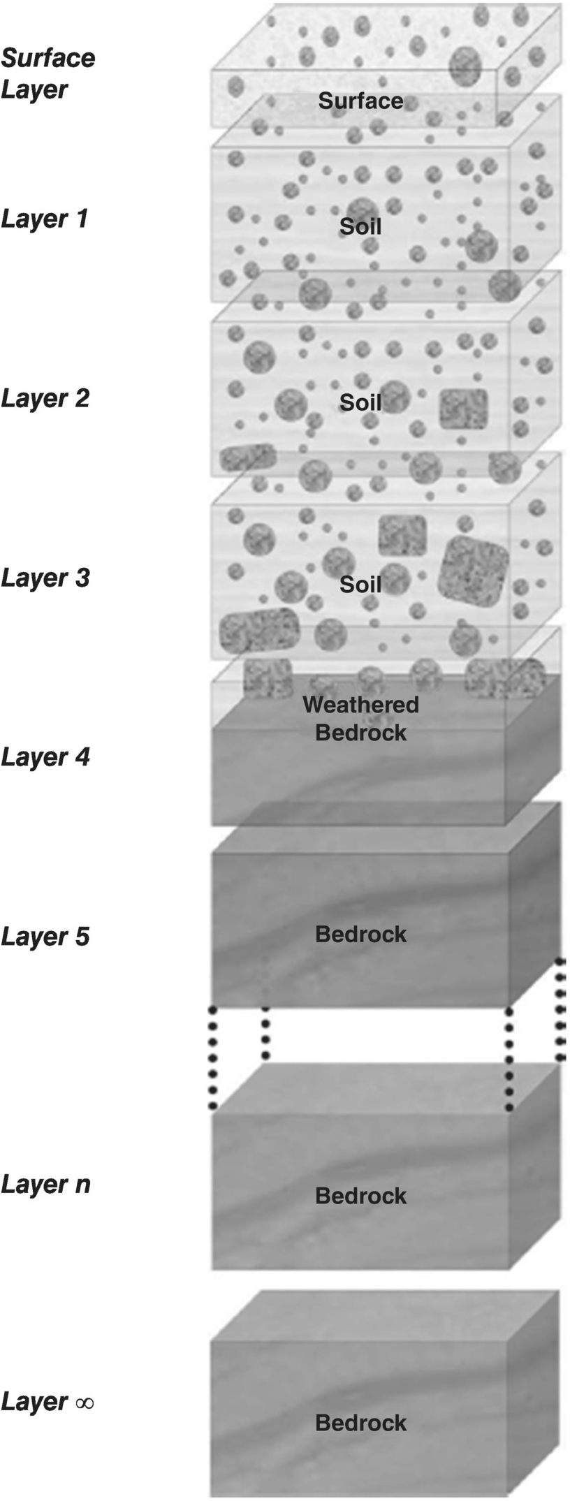
A soil profile is broken into a series of layers (Figure 7.1), with a thin layer on the surface that directly interacts with water flowing over the surface, and a semi-infinite layer of fractured rock underlying the profile. Each layer has a particle size distribution describing the mass proportion of each size within the soil grading. Pedogenic processes are modelled within each layer, and vertical interactions between the layers are modelled so that material can be moved between layers. To model a catchment the catchment is discretised into a spatial grid of nodes so that the catchment consists of a number of profiles, one profile for each node. Each layer is fully mixed vertically. Using the surface elevations of each node, the surface water drainage pattern is modelled and surface water flows from node to node. This surface water erodes and/or deposits sediment at each node based on the geometry of the surface flow network, the sediment being transported within the flowing water and the local transport capacity at that node. This used the erosion models discussed in Chapter 4. mARM3D ignores groundwater flows between the nodes (though, in principle, there is nothing to stop this being modelled), and there was no interaction between the soil layers at one node with the soil layers at another node. The main limits on the number of soil layers and the number of nodes spatially are computer storage and compute times.
7.3.1 Dynamics of a Single Soil Layer
We will first describe how mARM3D simulates each layer, and then we will discuss how the layers interact vertically. We start with the thin surface layer. This layer is the layer that interacts with the water flowing over the surface. In the most general case if the sediment transport capacity of the flow is more than the amount of sediment being carried by the flow, then the flow will erode material from the surface, while if the transport capacity is less than the sediment in the flow, then it will deposit sediment. If erosion occurs, then there is preferential entrainment of the finest fractions from the surface layer into the flow. To maintain the mass of the surface layer when there is erosion, material is transferred from the layer directly below to exactly balance the material being removed by erosion. If deposition occurs, then there is preferential deposition of the coarsest fractions (the coarsest particles settle out fastest) from the flow into the surface layer. To maintain the mass balance in the surface layer during deposition, material from the surface layer is transferred into the layer directly below to balance that material being deposited.
For the layers below the surface layer the mass balance is maintained at every time step. Thus if material is transferred from the layer to be put into another higher layer, then material is entrained from the layer below to balance the mass removed. Likewise if material is transferred into the layer from the layer above, then material from that layer is pushed down into the layer below. In the simplest case, if material is removed from the top layer by erosion, then material from the next layer below is transferred up to balance the mass lost to erosion. The next layer below that then has material transferred upwards to balance the material lost from the layer above, and this processes cascades down the profile to the bottom of the soil profile so that the soil-bedrock interface moves closer to the surface and the soil thins.
Within each layer weathering can occur and that weathering changes the grading distribution of that layer. Each layer weathers independently of the other layers. Mass conservative (i.e. physical weathering) and non-mass conservative (i.e. dissolution) weathering can be modelled, but to date full chemical weathering where dissolution is followed by precipitation of secondary minerals has not been modelled, because mARM does not have a coupled biogeochemical model to simulate in-profile geochemistry (Chapter 8). The weathering rate is typically depth dependent and can also be a function of particle grading and time. The model does not have a coupled groundwater model and so cannot model the effects of the interaction between soil moisture, soil grading and weathering rates, though a known, specified soil moisture spatial pattern (and thus a specified spatial weathering pattern) can be input.
The bottom layer of the soil profile has the grading of the underlying rock, rock being defined as material that is 100% the coarsest size fraction in the particle size distribution. That layer becomes soil as the weathering function breaks down the material into smaller size fractions. Any layers below cannot be soil until a specified proportion of the rock fraction in the layer above is broken down. Thus the bedrock-soil interface arises naturally as a result of the weathering process and is not explicitly modelled by the soil production function from Chapter 6.
Having outlined the conceptual approach used in mARM3D the mathematical details follow. The approach draws heavily from the state-space literature, and some of the terminology of this literature will be used where appropriate.
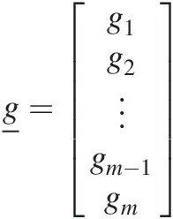
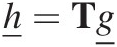
The soil grading at any given time and in any given layer is represented by a vector called the state vector 
 (7.2)
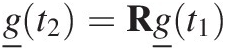
(7.2)and the entries in the state vector, gi, are the mass of sediment in each grading size range i where there are m size fractions for the grading. Cohen et al. (Reference Cohen, Willgoose and Hancock2010) used the proportion by mass of the layer in each size range as the state, but subsequent experience has found that using the actual mass in the layer in each size range makes it easier to apply mass conservation principles directly to the construction of the transition matrices (see below). The transition from the grading at any given time to the grading at the next time step is described by a matrix equation. It describes both how the grading changes with time and how the grading at one time, t1, is related to the grading at some time in the future t2:
 (7.3)
(7.3)where in the state-space literature the matrix R is called the transition matrix and is typically a function of the size of the timestep (t2 − t1). Note that any set of coupled differential equations can also be expressed with Equation (7.3). The advantage of the matrix formulation is that we can explicitly formulate all the processes that change the grading with the same methodology.
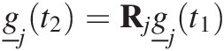
To represent the soil profile, we write one of these equations for each layer so that we can write Equation (7.3) for each layer down the profile, where Rj is different in each layer reflecting how weathering processes change down the profile. For each layer j we then have
 (7.4)
(7.4)The discussion in the remainder of this section will consider only what happens in a single layer, so we will drop the j subscript for the moment.
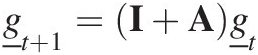
We simulate each physical process as a multiplicative change to the state. If we have a single process, let’s call it A, with a corresponding transition matrix R, then the evolution of the grading vector over one timestep is (using subscripts for the timestep)
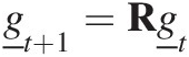 (7.5)
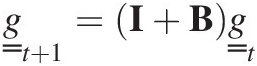
(7.5)which is simply Equation (7.3) where one timestep is (t2 − t1). To demonstrate how the method works for more than one process, consider the case where there are two independent physical processes, called A and B with corresponding transition matrices in Equation (7.5) of R and S; then the combination of these processes on the soil grading is
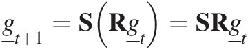 (7.6)
(7.6)where the order of the matrix multiplication implies that process A acts on the grading first and B operates second on the result of process A. This can be generalized to any number of processes, and is the key to the simplicity and generality of the approach. This splitting of processes into independent operations is ‘operator splitting’ (Section 2.2.2), and this splitting considerably simplifies the task of constructing the matrices for the combined effect of simultaneous physical processes.
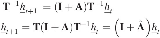
Equations (7.3) to (7.6) follow the traditional presentation of transition matrices. In the discussion that follows it is more convenient to work with the marginal transition matrix than the actual transition matrix. In this case
 (7.7)
(7.7)where I is the identity matrix (where  ) and A is the marginal transition matrix for process A. The change in grading over a timestep is proportional to matrix A. The advantage of formulating the matrices in this form is that the rate of the process represented by A (e.g. the weathering rate) can be changed simply by multiplying the marginal matrix by a scaling factor. For example, doubling the process rate is achieved by applying Equation (7.5) twice (the same as doing two timesteps), and if the timestep is small, then this is the same as multiplying the marginal transition matrix by 2 so that
 (7.8)
(7.8)where the A2 term is dropped since it is small for a small timestep. In the discussion that follows, the marginal transition matrix is used unless otherwise noted. In marginal transitional matrix form, Equation (7.6) is
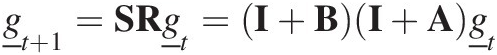 (7.9)
(7.9)where A and B are the marginal transition matrices for processes A and B, respectively, and correspond to the transition matrices R and S in Equation (7.6). Representing weathering and other processes within a layer is then a matter of constructing the marginal transition matrices and repeatedly applying the equations above.
Before we discuss how soil layers interact, a simple example will be useful to explain how the details of this process work. Consider an example where there are only three grading size ranges (for convenience let’s call them i = 1, 2, 3, ‘small’, ‘medium’ and ‘large’ grain sizes), and we will construct a marginal transition matrix for a weathering process that breaks large particles into medium particles, medium particles into small particles, and leaves the small particles unchanged. If at any one timestep 2% of the mass of the large particles are weathered into medium sized particles and 1% of the medium into fine, then the marginal transitional matrix is
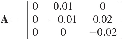 (7.10)
where the diagonal element says how much the mass changes in that grading range and the off-diagonal terms say how much of a different size range is added to it. For instance, for the medium (i.e. i = 2) size range
where 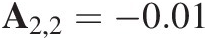 indicates that 1% of the mass in the medium size range is removed from it and
  indicates that 2% of the mass in the large size range is added to the medium size range.
Note that for mass conservation each column of the marginal transition matrix must add to zero. If mass is lost (e.g. by dissolution of particles), then the column(s) will sum to less than zero. Also note that none of the diagonal terms can be less than −1 because otherwise the equation is transforming more mass in the layer than actually exists in that layer. In this latter case a smaller timestep is required so that all the elements of the marginal transition matrix are smaller.
Finally it should be noted that, within the physical constraints above, there is considerable flexibility for the contents of the matrix, and therefore what processes can be simulated. The entries below the diagonal will normally all be zero because otherwise the process being represented by the matrix will be making larger particles from smaller particles (albeit if you are modelling soil aggregation or particle cementation this may be entirely reasonable). In the example in Equation (7.10) particles changed only to particles in the next size class down, which may not be the case, for instance, for particles that fragment into many smaller particles, or for spalling where there is a single large particle and many smaller particles resulting from the weathering. We will discuss these cases later.
While not presented this way the work of Salvador-Blanes et al. (2007) can be cast into this matrix formulation. Salvador-Blanes modified the approach of Legros and Pedro (Reference Legros and Pedro1985) to include the modelling of the breakdown of particles less than 2 mm in diameter and used Legros’s method whereby a particle was transformed into a particle in the next size class down (he defined that as 2 μm smaller). Both Legros and Salvador-Blanes used 1,000 size fractions for particles less than 2 mm, and this is easily transformed into Equation (7.10) (the A matrix will be 1, 000 × 1, 000) with only the diagonal terms and that entry directly above the diagonal term being nonzero, and the values being the rates at which one size fraction is transformed to the next smaller size fraction per timestep.
The recasting of Salvador-Blanes’s approach highlights an important but implied aspect of the matrix methodology. The matrix A is not describing how an individual particle is breaking down, but the aggregate result of the breakdown of the many particles in a size fraction. It is not possible to move a single particle to the next size class smaller and maintain mass conservation without generating some other smaller particles. However, the matrix method describes the aggregate of a given mass of particles, and it is possible to have many particles transform to the next size class lower without generating an array of fine particles.
7.3.2 Interactions between Soil Layers
We now describe how one layer within the soil profile interacts with another layer within the soil profile. Let us consider two layers j and k. We can construct a matrix equation that describes how layer j changes layer k in one timestep:
 (7.12)
This equation says how much mass in layer j in each of the grading size fractions is added to or subtracted from layer k in one timestep. Equation (7.12) models only how material is moved between layers and not weathering. We have used the matrix notation L here to distinguish this movement between layers from the weathering process matrices (that transform the particle size distribution within a single layer). For mass conservation in layer k, if mass is added to layer k from layer j, then an equal amount of mass must be removed from layer k and moved to another layer. The combination of the weathering and movement can be expressed in matrix form if we construct a grading vector that merges all the grading vectors for each of the individual layers, and the marginal transition matrix is constructed from the layer transition matrices and interlayer movement transition matrices so that
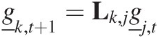
 (7.13)
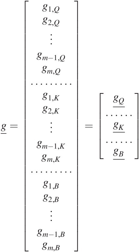
where the state vector is the gradings for all the layers from the surface armouring layer (subscript 1 indicates the surface armouring layer), through the profile layers and including the semi-infinite underlying layer (subscript ∞). The state vector is thus a vector of length m(n + 1) and the matrix is of dimension (m(n + 1)) × (m(n + 1)). The notation [0] indicates a matrix that is m × m and where all matrix entries are zeros. Equation (7.13) shows that all layers can interact with all other layers both above and below, including the semi-infinite underlying layer. Looking at the bottom row of the matrix, the semi-infinite layer can change through time (as a result of the matrix  ), but it cannot be influenced by any of the overlying layers (since all the entries are [0]). Equation (7.13) can be written in a more compact form
 (7.14)
where the double underbar notation distinguishes the grading vector for an individual layer (one underbar) from the vector for the gradings for all the layers (two underbars). The latter is sometimes called a supervector in the modelling literature (because it is a vector of vectors).
The construction of matrix B appears at face value to be rather daunting simply because of its size. However, Equation (7.13) is the most general statement of the problem, and in many cases simplifications are possible. For example,
If interactions between layers occur only between adjacent layers: In this case for layer j, the only matrices that are nonzero are the matrices
 for the weathering within that layer, and which describe how the layer above and below, respectively change layer j, and and which describe how layer j changes the layer above and below, respectively:(7.15)
If in addition to interactions only between adjacent layers, there is no change in the grading over time within a layer: This might happen when there is only mixing of the soil (e.g. bioturbation) and no breakdown of the mineral matter. The matrix in Equation (7.15) simplifies even further to
(7.16)Adjusting the layers in response to erosion at the surface: When material is removed from the surface layer, then material to balance that lost to erosion must be removed from the layer below to make sure the mass in the layer does not change. This cascades down through all layers in the profile:
(7.17)


where E is the erosion in one timestep in depth units, di is the depth of layer i (which converts sediment mass due to erosion E into a proportion of the layer mass) and I is a k × k identity matrix. The matrix A is the armouring transition matrix for the surface layer and determines the size selectivity of the sediment entrainment due to erosion. As an aside, this is the first time that bulk density of the soil appears in the matrix methodology. Bulk density is the conversion factor between depth of soil eroded and mass of soil eroded. If soil erosion is expressed in mass rather than depth units, then the bulk density conversion is not required.
7.3.3 Constructing the A Matrix for Weathering
We will now discuss how the matrix A is formulated to model weathering. Unless otherwise stated, the discussion in this section is for one layer, and we drop the layer subscript j for clarity of discussion. We will first discuss mass conservative weathering and then generalise the discussion to non-mass conservative weathering afterwards.
The basis of the conceptualisation of weathering is that particles are spread uniformly within each size range within which they fall (Figure 7.2). Thus some particles will be at the lower boundary of the size, some in the middle and some at the top of the size range. We conceptualise the fragmentation process as a parent particle breaking into a number of daughter particles (Figure 7.3). Figure 7.3 shows that depending on the fragmentation mechanism there may be a range of different types of daughter particles created. If we assume that the density distribution within a single particle size fraction is constant, then mass conservation implies volume conservation. In this case the total volume of the daughter particles is the same as the volume of the parent particle.
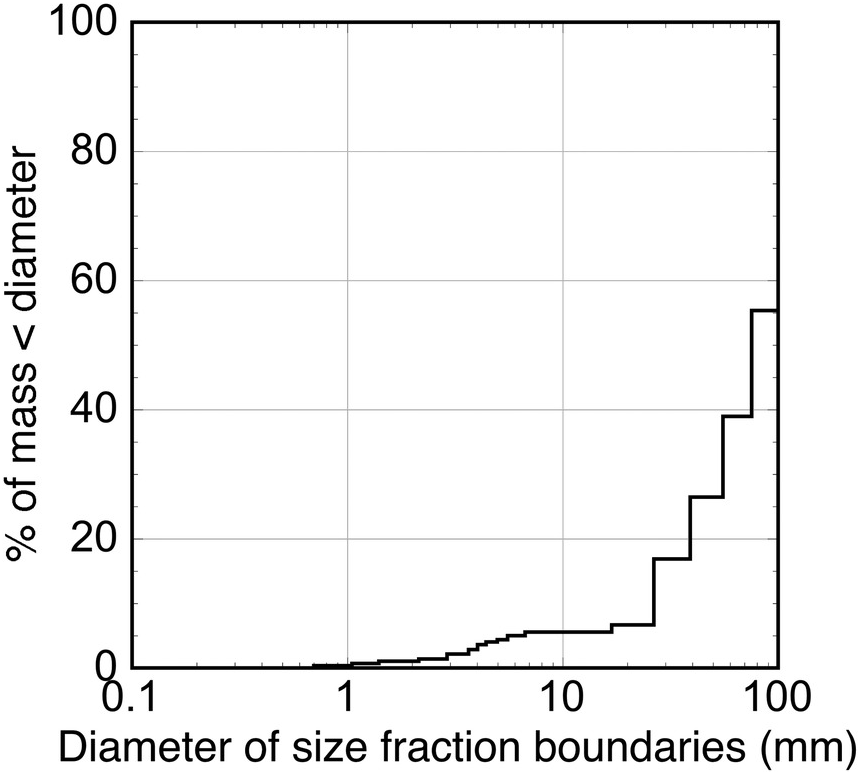
Figure 7.2: How soil grading is conceptualised in mARM and SSSPAM as uniformly distributed within size classes.
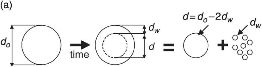
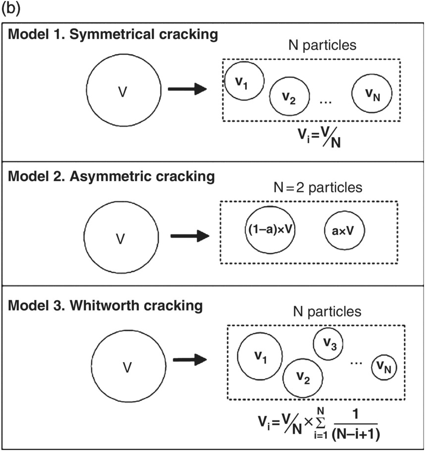
Figure 7.3: Schematic of fracturing models for rock particles (a) breaking of small particles from a rind and (b) body fragmentation.
We now extend our discussion from what happens to a single particle to what happens to all the particles within a size class range. Figure 7.4 shows what will happen to the larger size range when the particles break into two particles of different diameter, if they all follow the rules for breaking of a single particle (i.e. all particles break with exactly the same geometry). In the discussions that follow we assume that all particles are spherical. Initially we will consider the case where a parent particle breaks into two daughter particles. Figure 7.4 shows how the geometry of a single particle breaking allows us to map the parent particle size grade to the smaller dimensions of the two daughter particles’ size grades. Likewise we can map the largest size from the parent size gradings to the largest size of the daughter size grading. From the geometry of breaking of the single particle we know what the proportions of the mass of daughter particles should be in each of the two daughter particle gradings ranges. Figure 7.4 shows that if we take one parent size fraction, then the daughter particle’s size distribution will not typically neatly fit into a single size fraction, but will need to be interpolated across a number of size fractions. These proportions will be a function of the diameters of the daughter particles and of the size grading fractions adopted by the user in the modelling. Finally, if the distribution between the lower and upper size of the parent particles is uniform, then the distribution of the daughter particles is also uniform between the lower and upper size grading.
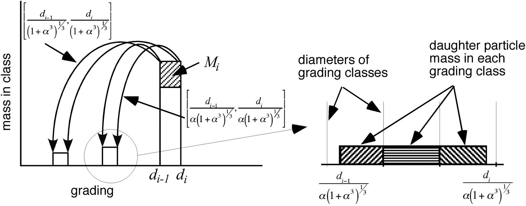
Figure 7.4: Conceptualisation of how size fractions in the grading are transformed in each time step of mARM.
Using these assumptions it is relatively straightforward, though tedious, to construct a matrix to simulate weathering. The calculations in Figure 7.4 are done for each grading range and the results summed.
However, a conceptual simplification is possible. There is a combination of grading size fractions and weathering processes that leads to particularly simple results, and which allow us to derive some analytical results that provide useful insight into the time variation of grading under the action of weathering. We will use this to demonstrate how the weathering matrix works and derive some simple weathering results. We will then show that this simple model can be used to derive more complex models.
For this example we will define the fractions in the grading size distribution such that the lower diameter limit of each size fraction is 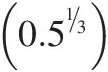 times the upper diameter limit for that same size fraction. If we take the maximum size limit as 2 mm, then this yields the limits for the size fractions as in Table 7.1. There is no special significance to the upper and lower limits of 2 mm and 0.125 mm in the table; they are simply used to show what this grading looks like. It is useful to examine this size grading because this grading fractionation is different from that normally used for soils analysis (e.g. phi grading) and thus will be unfamiliar to readers. The significance of the grading in this example is that if a spherical particle splits into two equal volume spherical daughter particles, then for conservation of volume all the particles in one size grading will fall exactly into the size grading of the next size fraction smaller. For example, for the grading class 12 in Table 7.1 a particle with the largest diameter of 2 mm will split into two particles of diameter 1.587 mm, and a particle with the smallest diameter of 1.587 mm will split into two particles of diameter 1.260 mm. These upper and lower size limits define the size range for the next smaller Grading Class 11. This is true for all Grading Class ranges in Table 7.1.
Table 7.1: Size grading classes for different weathering mechanisms for two equal particles and three equal particles fracturing
| Size grading class | Upper-lower size limit (mm) | |
|---|---|---|
| 2 daughters | 3 daughters | |
| 12 | 2.0–1.587 | 2.0–1.387 |
| 11 | 1.587–1.260 | 1.387–0.962 |
| 10 | 1.260–1.000 | 0.962–0.666 |
| 9 | 1.000–0.794 | 0.666–0.462 |
| 8 | 0.794–0.630 | 0.462–0.321 |
| 7 | 0.630–0.500 | 0.321–0.222 |
| 6 | 0.500–0.397 | 0.222–0.154 |
| 5 | 0.397–0.315 | 0.154–0.107 |
| 4 | 0.315–0.250 | 0.107–0.074 |
| 3 | 0.250–0.198 | 0.074–0.051 |
| 2 | 0.198–0.158 | 0.051–0.037 |
| 1 | 0.158–0.125 | 0.037–0.025 |
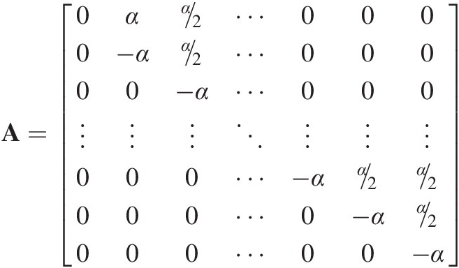
Accordingly, to assemble the weathering matrix with this grading when a parent particle fractures into two equally sized daughter particles is straightforward because the daughter particles only ever fall into the size fraction below, and this size fraction below can receive only daughter particles that fracture from the size fraction directly above. Thus if we say that the proportion of the particles that fracture for one timestep is α, then the weathering matrix is
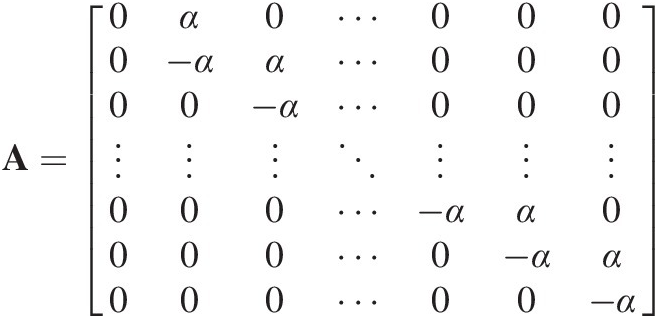 (7.18)
The diagonal and off-diagonal α terms mean that α of the mass in the larger size grading is all added to the next smaller size grading. The diagonal element for the smallest fraction is zero because we assume that particles this size cannot weather any smaller. Equation (7.18) is mass conservative, so all the columns of the matrix add to 0.
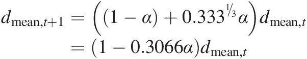
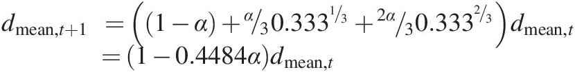
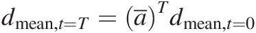
It is possible to calculate the time variation of the mean diameter of the particle size distribution purely from the I + A matrix using Equation (7.18). With the exception of the smallest size grading, the mass gi that is in any given size fraction i will change after one timestep so that (1 − α) remains in size fraction i while α will now be in the next size fraction smaller i − 1, which in the case of Equation (7.18) is  smaller than the size fraction above, and from the way the size fractions are defined in Table 7.1 that is true for all size fractions i. For the smallest size fraction there is no change. If we consider the case where all the mass is initially concentrated in the largest size fractions and there is an insignificant mass in the smallest fraction (this can be achieved by defining the smallest size fraction to be very small), then in one timestep (time changing from t to t + 1) the mean diameter of the soil changes from
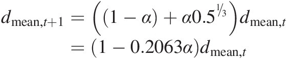 (7.19)
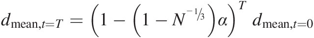
which allows us to derive an equation for the evolution of the mean diameter of the soil T timesteps into the future:
which is a semi-log linear relationship between diameter and time, where the slope on a semi-log plot is −0.2063α. This can also be expressed as an exponential so that
Figure 7.5 shows this curve for a number of values of α and with a starting mean diameter of 3.5 mm.
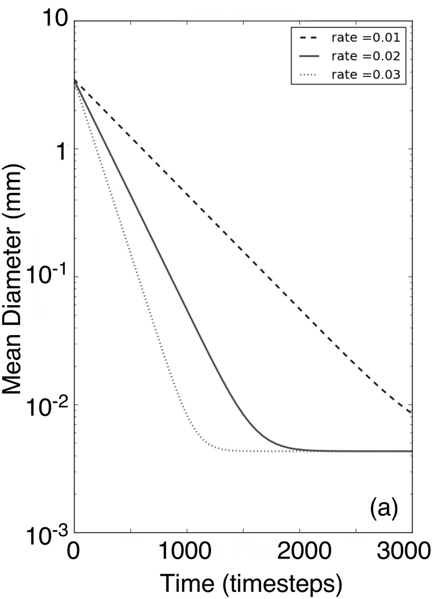
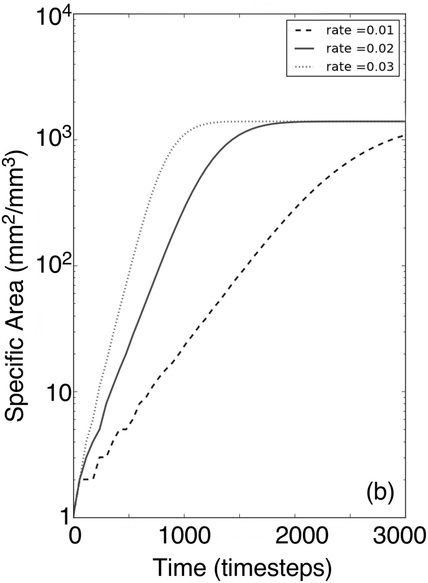
Figure 7.5: Numerical solution of the time evolution of the mean of the particle size distribution for a range of weathering rates. The parameter ‘rate’ is rate = 0.2063α in Equation (7.19). The levelling off on the right-hand side of each graph is because at this stage all soil is in the finest size fraction in the modelled soil grading.
The exact details of Equations (7.19) to (7.21) are a function of the specific assumptions in Equations (7.18), but it is straightforward to extend this analysis to any distribution of daughter products, and the only part of Equation (7.19) that will change is the number inside the parentheses; the relationship itself will still be log-log linear. This is true provided only that (1) the definition of the size fractions is defined as in Table 7.1 for two daughter particles, (2) the fracture model is independent of the diameter of the particle so that the daughter particles are always the same size relative to the parent particle and that this fracture model is independent of the diameter of the parent particle and (3) the smallest size fraction is small enough that only a minor amount of the mass occurs within the smallest fraction (otherwise the curves will start to level out as the particles age as seen in Figure 7.5 on the right-hand side).
The assumption that particles split into two equally sized particles leading to Equation (7.21) is rather restrictive, but this result can be generalised as follows. Consider first the case where N equally sized particles are generated at each time step instead of the two in the example above. This means that the diameter of the daughter particles is now  the diameter of the parent particle. In the same way that we developed a grading range definition for two daughter particles fracturing in Table 7.1, we can do this in general for all values of N. In Table 7.1 fracturing for three equal daughters is shown. Note that the total size range covered by the 12 size fractions in Table 7.1 is different, with the three daughters column going down to 0.025 mm, while the two daughters range goes down to only 0.125 mm. Thus if you wish to cover a specific total size range (e.g. for a given soil), the two daughters size range requires more size fractions. If the proportion of a given size fraction that breaks down each timestep is α as before, then Equation (7.18) is still applicable except now the definition of the size grading ranges is different and the matrix will be of a different dimension. The equivalent three daughters result to Equation (7.19) is
 (7.22)
and Equation (7.20) becomes
In general for N daughter particles
 (7.24)
so it is clear that if particles break into a larger number of smaller particles at each timestep, then the soil will become finer at a faster rate, and Equation (7.24) defines what that speedup will be.
In the discussion that follows we further generalise the fracture geometries considered. To simplify the discussion of geometry we introduce a shorthand for fragmentation geometry, which indicates how, on average, the volume of particles will be distributed after a fragmentation event assuming the size grading definitions in Table 7.1. The general form is pX-AAA-BBB-CCC-DDD where X is the number of daughter particles the grading fractions have been defined for (i.e. X = 2 for the two particle grading in Table 7.1, X = 3 for the three particle grading), AAA is the percentage of volume that remains in the parent size grading fraction after fragmentation, BBB is the proportion in the next size grading smaller, CCC in the next size down again and so on. In this notation where all of the particles split into two with two equally sized particles, then the shorthand is p2-0–100. Some geometry examples are listed in Table 7.2. Some simple examples of fracture geometries and their fragmentation notation are also shown. While all the examples in Table 7.1 have no mass left in the parent grading after fragmentation (they all have a leading zero), at the end of this section an important, but more complex, fragmentation geometry that leads to a nonzero percentage in the parent grading will be discussed.
Table 7.2: Fragmentation notation examples
| Fragmentation notation | Physical example for daughter particle geometry |
|---|---|
| p2-0–100 | 2 particles of 50% volume of parent. The split in two geometry of Wells et al. (Reference Wells, Willgoose and Hancock2008). |
| p2-0–50-50 | 1 particle of 50% volume, and 2 particles of 25% volume of parent. |
| p2-0–50-0–50 | 1 particle of 50% volume, 0 particles of 25% volume and 4 particles of 12.5% volume of parent. Spalling-like behaviour. |
| p2-0-0-0–100 | 0 particles of 50% and 25% volume, and 8 particles of 12.5% volume of the parent. Used by Finke (Reference Finke2012) in the SOILGEN model. |
| p2-0–50-25-12.5-12.5 | 1 particle of 50%, 1 particle of 25%, 1 particle of 12.5% and 2 particles of 6.25% volume. A scaling fracturing similar to Whitworth cracking (Figure 7.3). |
Instead of two equally sized daughter particles, let us now break the particle into three daughters where one daughter is half the volume of the original and the other two daughters are a quarter of the volume of the original (i.e. p2-0–50-50). Mass conservation still applies, but what now happens is that half the weathered volume goes into the next class down from the parent, while half the weathered volume goes into the class 2 classes below the parent so the A matrix is
 (7.25)
and Equation (7.19) becomes
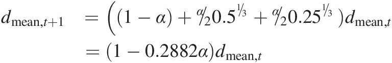 (7.26)
As expected this case weathers faster than the two equal daughters case. In a similar fashion you could consider that this three daughters case can be extended where one of the two smaller particles itself breaks into two, so the daughter particles are 1 × (1/2) volume, 1 × (1/4) volume and 2 × (1/8) volume and so on.
Similarly the three equal daughters particle fracturing could be extended by having one of the daughters break into three equal volume smaller particles, so that the daughters are two particles with 1/3 the parent volume (i.e. 2/3 of the parent volume) and three particles with 1/9 the parent volume (i.e. 1/3 of the parent volume), yielding p3-67.7-33.3. In this case Equation (7.25) becomes
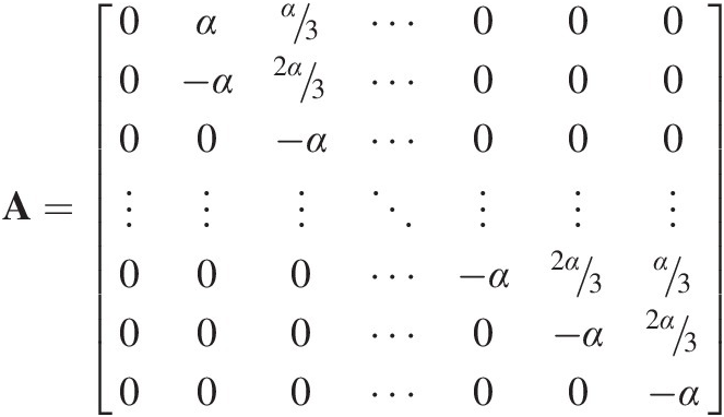 (7.27)
and Equation (7.26) becomes
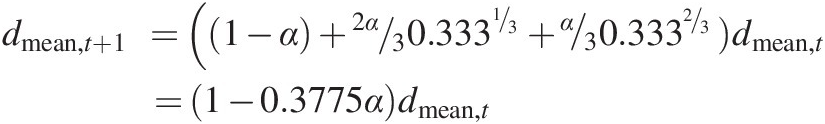 (7.28)
If two of the three daughters break into three (i.e. p3-33.3–66.7), then
 (7.29)
and as for the two daughters cases, both of these cases weather faster than the case where all the daughters are of equal sizes, and when more fine particles are generated (i.e. Equation (7.29) versus (7.28), or Equation (7.28) versus (7.26)) then the soil weathers faster even when the rate of breakdown per timestep is unchanged.
It should be clear from these examples that the combinations of sizes of daughter particles possible are quite extensive. The only constraint is a geometry constraint driven by the grading size definition adopted from Table 7.1. If the two daughter grading range in Table 7.1 is adopted, then particles must break into particles where the volumes of the daughters are related to the parent particle volume by integer powers of 1/2. Likewise for the three daughter grading range in Table 7.1, then all the daughters must have volumes that are integer powers of 1/3. This integer power constraint is so that all the daughters fall entirely and only into one of the grading size ranges and do not span two grading size ranges.
This section has shown how to construct the weathering A matrix using a conceptualisation of the fracturing of individual parent particles into a range of daughter particles. Thus everything in this section has been strongly physically based on fracturing mechanisms that are, in principle, observable in the laboratory or the field. This presentation was intentional because it highlights the link between fracturing of individual particles and the rather less tangible mathematics of the A matrix.
We will deviate from this philosophy for a moment to generalise Equation (7.18), which will then allow us to provide a general analytical solution to the change in grading over time. When constructing the A matrix, to ensure mass conservation we need to ensure only that (1) the summation of each column should be zero, (2) the diagonal term is between −1 and 0 and (3) the off-diagonal terms are greater than or equal to 0. Thus if we can construct a generic column for matrix A, that is the same for all grading fractions
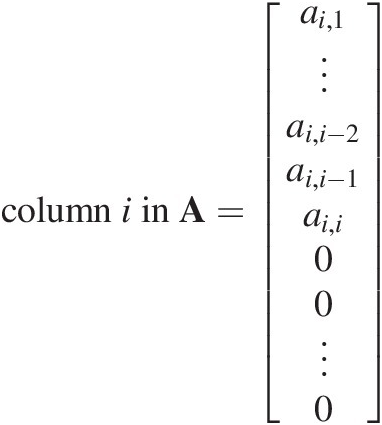 (7.30)
we can then write Equation (7.19) as (using the two daughter size grading)
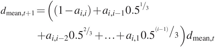 (7.31)
and if the values of ai, j are small when j is small (i.e. large parent particles do not generate many very small daughter particles), then we can write
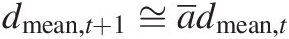 (7.32)
where  is a constant reflecting the structure of A so that we can write a general equation for how the mean diameter of the soil will change over time
 (7.33)
which shows that the mean of the soil grading is an exponential function with time of the initial grading irrespective of the structure of A. Note that the restrictions on the form of A are relatively modest (just that weathering cannot generate a large mass proportion of small particles), so this is quite a powerful and general conclusion. Note also that the use of the two daughter size fraction definition in Table 7.1 is a convenience rather than a necessity, as we will see in the next section. The fragmentation notation for this case is p2-(1-ai,i)-ai,i-1- … -ai,1.
The discussion above presumes that all particles fracture with exactly the same geometry. This is not essential. One simple extension is to allow particles to break with two possible geometries at different rates. The A matrix for the combined process is then
 (7.34)
where the subscripts are the weathering rate w and weathering matrix A for each of the two processes. This can be generalised to as many processes as required.
Figure 7.6 extends the discussion by examining a number of fracture geometries, and shows how (1) the different fracture geometries yield different rates of evolution of the mean grading and (2) all the geometries evolve as a semi-log of time as in Equation (7.33). The meaning of the coding used for describing fracture geometry is explained in the figure caption, but is based on the fracture geometry where particles are 1/2, 1/4, 1/8 and so on of the volume of the parent particle.
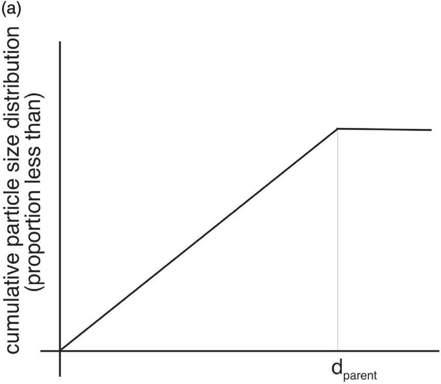
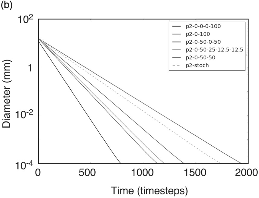
Figure 7.6: (a) The average particle size distribution of the daughter particles resulting from random fragmentation (P2-stoch), dparent is the diameter of the parent particle, (b) Numerical solution of the time evolution of the mean of the particle size distribution for the same weathering rate (as used in Figure 7.5) and a range of fragmentation models. The weathering model p2-0–50-50 is the same as ‘rate = 0.03’ in Figure 7.5.
One of the fracture geometries in Figure 7.6 is philosophically different from the ones described above. In all the fracture geometries above the geometry of the daughter particles is deterministically fixed as a proportion of the volume of the parent particle. The aggregated behaviour of all the particles is then just the sum of all the particles in that grading range. However, consider the case where a single particle breaks into two particles but where the fracture location in the particle is randomly distributed within the particle (e.g. a schist where the particle cleaves along the layering but where the cleavage plane is randomly located within the particle). The probability distribution of the volume of daughter particles derived from particles in a specified particle range is shown in Figure 7.6a. It is convenient here to define the x axis as the volume of particles rather than their diameter because the probability distribution of the daughter particles is then particularly simple. If a large number of particles fracture, then the probability distribution function gives the mean of the volume distribution of the daughter particles, from which A can be easily derived. In fragmentation notation it is p2-30.7-34.6-17.3-17.4, if we lump the volume of all particles more than three grading fractions smaller into the third grading fraction (i.e. the 17.4). Other than the proportion remaining in the parent grading range, the relativities between the daughter size fractions are the same as the scaling model p2-0–50-25-12.5-12.6.
Figure 7.6 shows that those fractions that generate a greater proportion of volume in smaller size fractions fine faster, which is consistent with Equation (7.24). Figure 7.7 shows the particle size distribution resulting from using a number of different fragmentation models. Initially all particles were 4.0 mm in diameter, and Figure 7.7 shows the particle size distribution when the fragmentation models have weathered the particles to a median diameter 0.1 mm. Two conclusions of this figure are that (1) different fragmentation models yield slightly different particle size distributions even though the median diameter of the particle size distribution is the same and (2) while the different fragmentation models may yield finer particle size distributions at different rates, they yield particle size distributions that are only slightly different (e.g. the p2-0–100 and the p2-stoch random fracture models are indistinguishable in Figure 7.7, but p2-0–100 fines a factor of two times faster in Figure 7.6).
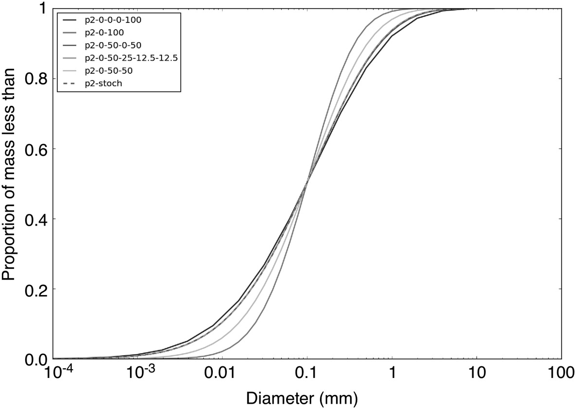
Figure 7.7: These are the same simulations as in Figure 7.6 (i.e. same weathering rate, different fragmentation models) but showing the particle size distribution when the d50 of the all fragmentation models is equal to 0.1 mm. Note that Figure 7.6 shows that the age of each of the distributions will be different since the different fragmentation models generate a different rate of change in the d50 for the same weathering rate.
7.3.4 Transforming the Size Grading Definition
The definition of the size fractions necessary to derive Equations (7.18) to (7.29) is rather restrictive, and is not necessarily consistent with size gradings used in soil science practice (e.g. sieve sizes). Accordingly, we will now show how to generalise the definition of diameters defining the size fractions while still maintaining the simplicity of the equation and the semi-log relationship for mean size with time. It is possible to transform the mass fractions from one size fraction definition to another size fraction definition. Consider  to be the grading by one grading class size definition and
  to be the desired mass fraction equivalent to
  in another grading class size definition. For generality let us consider that there are n size classes in
  and m size classes in
  . We can transform
  into
into  with the matrix equation
 (7.35)
where T is a n × m matrix that distributes the mass in the n classes in  into the m size classes in
  .
.
We can now transform the weathering (or any other process for that matter) matrix equation that is originally
 (7.36)
By substituting in the inverse of Equation (7.35) we get the transition matrix in the new grading
 (7.37)
so that in the new grading definition
 (7.38)
noting that 
This shows that we can populate the A matrix using any size class definition we like and then later transform it into any other size class definition that is convenient. One major consequence of this is that the semi-log evolution of the mean diameter we have derived in the previous section is not unique to the size class distribution used to derive it, and that even if the class definition is different (provided the physics is the same), then the semi-log relationship with time will still be observed.
7.3.5 Constructing the A Matrix for Pedoturbation
Pedoturbation is any process that disturbs the horizonation of soils. Some pedoturbation processes assist in the differentiation of soils into layers, while others mix the soils, tending to destroy the layers (Hupy and Schaetzl, Reference Hupy and Schaetzl2006). Bioturbation is a pedoturbation process resulting from biological activity and is a significant process in soil profile development (Hole, Reference Hole1981). One of the main impacts of bioturbation is to physically mix soil from top to bottom (Heimsath et al., 2002; Ahr et al., Reference Ahr, Nordt and Forman2013), and transport material from the surface into the profile (Astete et al., Reference Astete, Constant, Thibodeaux, Seals and Delim2015). Soil fauna such as ants and termites bring fine material from deep in the soil to the surface (Lobry de Bruyn and Conacher, Reference Lobry de Bruyn and Conacher1990), earthworms likewise mix the profile (Van Hooff, Reference van Hooff1983; McKenzie et al., Reference McKenzie and Dexter1993), while tunnelling animals such as gophers (Huntley and Inouye, Reference Huntly and Inouye1988; Gabet, Reference Gabet2000) and wombats (Paton et al., Reference Paton, Humphreys and Mitchell1995; Field and Anderson, Reference Field and Anderson2003) may also transfer material laterally (via their horizontal tunnels) as well as from within the profile to the surface. Flora such as trees mix the soil through tree throw (Gabet et al., Reference Gabet and Dunne2003; Field and Anderson, Reference Field and Anderson2003). In this section we will consider only vertical transport of material. Horizontal movement will be discussed in Chapter 9.
Many of these processes leave macropores within the profile when material is removed from that layer, which means that the porosity is increased and the bulk density of the soil layers is reduced. If the mass in each soil layer in the model is the same and bulk density decreases, then the layers will dilate (or expand), so that the soil surface rises. For instance, Wilkinson et al. (Reference Wilkinson, Richards and Humphreys2009) provides data for bioturbation rates that decline with depth roughly exponentially from the surface, which they attribute primarily to ants and worms. They also measured bulk density and found increases with depth (1.1 g/cm3 near to the surface to 1.8 g/cm3 at a depth of 0.8 m) mirroring the decline in the rate of bioturbation and number of macropores generated. Shull (Reference Shull2001) presents a very similar matrix model for bioturbation in sea bottom sediments.
One unusual form of pedoturbation was the soil mixing resulting from artillery shells in France during World War I (‘bombturbation’, Hupy and Schaetzl, Reference Hupy and Schaetzl2006, Reference Hupy and Schaetzl2008), and these and other warfare sites provide unique field experiments in pedogenesis (Certini et al., Reference Certini, Scalenghe and Woods2013).
7.3.5.1 Simple Biological Mixing
A simple model for bioturbation mixes the soil vertically randomly, and this can be modelled as a vertical diffusive process. The idea is that microfauna (e.g. earthworms) mix the soil vertically. This process could be modelled by a Fickian diffusion-type equation. A simple method, which asymptotes to Fickian diffusion (i.e.  where Qs is the rate of vertical transport per unit area and time,
  is the gradient of the property C being mixed and D is the diffusivity), is to exchange material with the layers above and below (Williams, Reference Williams2006):
 (7.39)
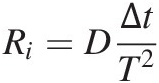
where Ri is the rate of bioturbation mixing at the depth of layer i. Equation (7.39) assumes that all layers have the same thickness. Following Wilkinson et al. (Reference Wilkinson, Richards and Humphreys2009) the bioturbation rate Ri declines with depth approximately exponentially. The identity matrix I means that the mixing is not size selective. For constant thickness T layers, this converges to Fickian diffusion asymptotically with time
 (7.40)
If the layers are of different thickness, then the ith column of tridiagonal elements changes to
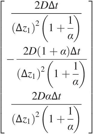 (7.41)
where (see definitions in Figure 7.8) Δz1 is the distance between the nodes i and i − 1, Δz2 is the distance between nodes i + 1 and i, and  . The relationship in Equation (7.41) is derived from a central finite difference approximation to Fickian diffusion. When the thicknesses of the three layers are the same (i.e. Δz1 = Ti and α = 1) Equation (7.41) reduces to Equation (7.40).
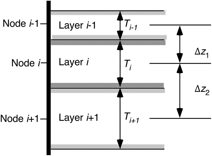
Figure 7.8: Definitions of layer thickness and node discretisation for Equation (7.41).
7.3.5.2 Tree Throw
Tree throw brings to the surface all the soil in the root ball of the tree leaving behind a large hole in the ground. The soil falls off the roots over time, and the mixed soil in the root ball refills the hole in the ground. In addition to the mixing, there is potentially an impact on the porosity of the soil with the soil becoming more disordered. Tree throw is an event: a tree falls, and the consequences happen immediately. It is not a slow ongoing process, though the cumulative impact of many tree throw events is an ongoing process. Tree throw can be modelled as an event if it is assumed that the refilling of the hole happens quickly relative to the timestep of the modelling. At a given time a tree falls at a particular location or it doesn’t. Thus we do not use Equation (7.14) as the model of what happens from t to t + 1, but we can use it to model what happens before and after the tree fall event
 (7.42)
We simply need to know, when a tree fall event occurs, what the B matrix looks like for a single tree fall event, and apply Equation (7.42) for that time (and apply the equation repeatedly if there are many tree fall events at the same time). The mixing of the soil over the depth of the root zone is modelled using Equation (7.42) if we assume that the root ball rips up the top n layers so the top n layers are mixed together and the n + 1 and lower layers are undisturbed. This is an averaging of the grading of the top n layers so that the B matrix can be expressed as
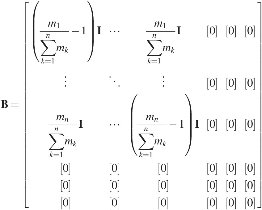 (7.43)
where mj is the total mass of layer j. The zero matrices for i greater and equal to n + 1 indicate that the tree throw does not change the grading for layers n + 1 and deeper. The term  is included to ensure that the mass in layer j is the same before and after the tree fall event. This is not critical but is convenient, because it preserves the thinner armour layer, which would otherwise become the same thickness as the underlying layers if the mass were distributed equally. The −1 in the diagonal term ensures that the grading in that layer is entirely replaced by the new grading to negate the effect of the identity matrix in Equation (7.42).
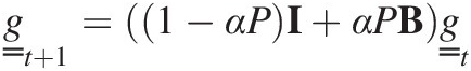
When modelling soil spatially it will often be the case that a single tree throw event disturbs only a proportion of the area associated with each computational node. If we call this proportion α, then the equation for that node is a modification of Equation (7.42) so that
 (7.44)
where the (1 − α) term is the proportion of the nodal area that is unchanged by the tree throw event while the α term is that proportion of the nodal area impacted by tree throw. The parameter α might change from tree throw event to tree throw event reflecting the size of the tree (and thus the root ball) impacted. Likewise the depth of mixing might change between events to reflect tree throw for different size trees.
When modelling the temporal effect of tree throw (i.e. over a number of years rather than over a single tree throw event), there are two main alternative approaches.
The first approach is to model tree throw as occurring randomly in time and space (i.e. a Poisson random process) and modelling every tree throw event using the equations above. If tree throw has a probability of occurring of p per unit area per timestep, then the probability P of a tree throw event in a given timestep in a node of area A is P = pA. The simplest way to simulate this is to cycle through every node at each timestep and randomly generate a uniformly distributed random number between 0 and 1 for each node. If the random number is greater than P, then a tree throw event occurs in that node, while if it is less than P, a tree throw event does not occur. If the area of a node is large, and/or the timestep is long, then it is possible for P to be greater than 1 (which indicates more than one tree throw event). In this case either one of the timestep or node area needs to be decreased.
The second approach calculates the average effect of tree throw over many events and models the mean behaviour rather than the effect of individual events. In this case the mean of the tree throw events in any given node is the rate of tree throw occurrence per unit time, which is P, so that the equation for the effect of tree throw per unit time, by modifying Equation (7.44), becomes
 (7.45)
The advantage of the first method is that you can capture the stochastic effect (in both space and time) of tree throw, whereas the second method gives only the average effects. This stochastic effect may be important in the understanding of the spatial variability of the soil properties (e.g. Samonil et al., Reference Samonil, Kral and Hort2010; Gabet and Mudd, Reference Gabet and Mudd2010). The average of the first method gives the second method.
Because both these methods independently examine each node, the user can impose spatial variability on tree throw reflecting that tree throw is spatially clustered around the edges of forests and in openings within the forest, and that throw events are clustered in time during high-wind events. In this case the user can construct a wind event model, where wind is randomly generated across the domain, and based on the wind speeds impose a spatial pattern of tree throw occurrence (e.g. Espirito-Santo et al., Reference Espirito-Santo2014) and study its effect on the spatial variability of soil development (Finke et al., Reference Finke, Vanwalleghem, Opolot, Poesen and Deckers2013).
7.3.5.3 Termites and Ants
Termites and ants move fine soil material from the subsurface to the surface as part of nest construction (Paton et al., Reference Paton, Humphreys and Mitchell1995; Zaitlin and Hayashi, Reference Zaitlin and Hayashi2012). The surface expression of these nests is then, over time, eroded (typically by rainsplash) so that the material moved to the surface of the nest is then spread as a surface veneer over the soil surface, over an area that might be larger than that contained by the nest itself. The underground galleries of the nests are the material that is moved to the surface and may be quite extensive laterally (e.g. termite nests may extend 10’s of metres laterally) and vertically. Neither the lateral nor vertical density of the galleries is well defined (and likely to be species, climate and soil specific), nor is the spatial distribution of nests (all of which determine the mass of material moved). This also applies to the length of time before the galleries collapse and the soil above them subsides (which determines the rate of change of the porosity of the soil in those layers that contain the galleries).
The general principle here is that soil with a given size grading range (though the evidence for size selectivity for ants is not definitive, and nest-building behaviour appears to be strongly species dependent; Lobry de Bruyn and Conacher, Reference Lobry de Bruyn and Conacher1990, Reference Lobry de Bruyn and Conacher1994) is removed from each subsurface layer and deposited on the surface. To ensure that the mass in each layer does not change, we transfer material down from each overlying layer into the layer below until we reach the bottom of the bioturbed region. First, we will look at how to calculate the amount and grading of material transported to the surface by the ants. So for layer i the material removed is
 (7.46)
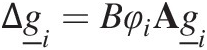
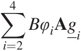
where  is the change in the soil grading vector in this time step, B is the rate constant determining the total amount of material transported to the surface (not to be confused with B the matrix), φi is a normalised function of depth describing the relative rate at which material is transported from each layer i (i.e. φi is the depth dependency of ant-turbation) and matrix A is a normalised matrix describing the size selectivity of the ant-turbation mechanism. An example of matrix A is
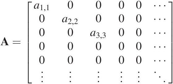 (7.47)
where the diagonal elements aj, j are the proportion of the total mass in grading size range j that is transported upwards by the bioturbation (i.e. aj, j = 0 if nothing is removed, aj, j = 1 if it is all removed). In this example a4, 4 = 0 because for grading size range 4 it is assumed that none of that size range is transported upward (e.g. because it is too coarse). I have shown only the first five rows and columns of the matrix for brevity.
It also turns out to be convenient to define the total mass (i.e. across all grading size classes) in layer i, mi, and the total mass of the change in the soil grading vector for layer i, Δmi,
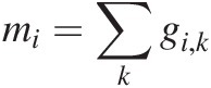 (7.48)
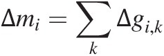 (7.49)
where the subscript i indicates layer i and the subscript k is the kth grading class in layer i.
For simplicity of explanation let us consider a case where the ant galleries are excavated in the top four layers, and the layers below are untouched. Then material will be excavated from layers 2 through 4 and deposited into layer 1. To ensure that the mass in each of the layers is unchanged, we then need to transfer the excess material in top layer down into layer 2, from layer 2 to layer 3 and so on. (Figure 7.9). The mass and grading of the material brought to the surface is
 (7.50)
The fluxes of soil between the layers are given in Figure 7.9 and are based on a fully explicit numerical representation of the process where each of the soil layers is fully mixed. Importantly in Figure 7.9 the grading of the material from one layer to the layer below is based on the grading of the layer prior to the redistribution of the soil into the layer above. This is the explicit numerical approximation of the time discretisation. There is no conceptual reason why the derivation can’t use the grading in the layer above after the soil has been redistributed to it; the arithmetic in the equation below is just more complex.
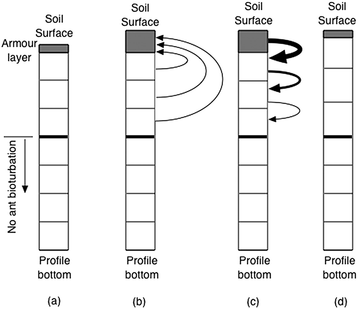
Figure 7.9: Schematic of how layers interact in ant and termite bioturbation. While the calculations are done using mass, the figure shows the layer thicknesses: (a) the soil profile before ant bioturbation, including the thin surface armour layer, (b) the movement of material by ants, from the top three layers into the surface armour layer (those layers above the thick line are subject to ant transport, those below not; the grey region is the surface armour layer; note that the only layer that changes thickness is the surface armour layer, so the bulk density in the lower layers is reduced), (c) the redistribution of excess sediment from the surface armour layer (the thickness of the lines and arrows indicate quantities of soil being moved between layers) and (d) the reinstatement of the armour layer, which is now a mix of the original armour layer and the ant transport material. The soil surface has risen because of the reduction of the bulk density of the layers from which ants removed materials.
We can write the equations for the new grading in each of the four layers. Starting at the surface and working down the profile,
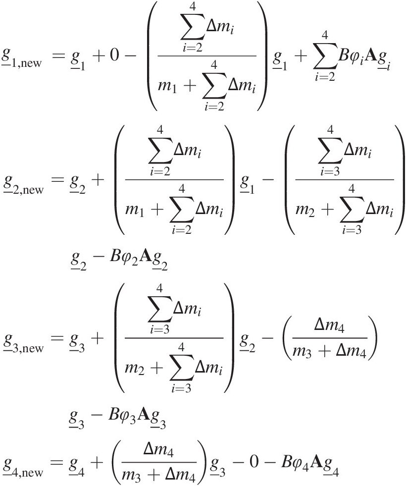 (7.51)
where the first term on the right-hand side of each equation is the grading before ant-turbation, the second term is the soil being transferred down from the layer above, the third term is the soil being transferred down to the layer below and the fourth term is the material moved by the ants/termites. The zeros in two of the equations are placeholders so that the third and fourth terms are the same processes in all four equations. Constructing the transition matrix from these equations involves filling the matrix according to Equation (7.51):
 (7.52)
where, for brevity, only the first five rows and columns of the transition matrix are shown.
7.3.5.4 Gophers, Wombats and Prairie Dogs
Burrowing animals also move material from within the profile to the surface. There are strong similarities between the ant/termite representation in the previous section and that for larger burrowing animals. The main differences are (1) the size and extent of the tunnels, (2) the size selectivity of the material excavated and (3) that there tends to be more lateral (either across or up/down slope) movement of material because tunnels are predominantly horizontal.
In North America pocket gophers are an important mechanism for laterally moving soil (Gabet, Reference Gabet2000) impacting on vegetation (Huntly and Inouye, Reference Huntly and Inouye1988). Their burrows extend up to 100 m laterally though they do not dig very deep (<1 m). It thus seems reasonable to assume that they would also mix the soil vertically (Hole, Reference Hole1981), though there is less quantitative literature on this possible impact (Gabet et al., Reference Gabet and Dunne2003).
In a review of bioturbation in North American soils Zaitlin and Hayashi (Reference Zaitlin and Hayashi2012) concluded that prairie dogs had a significant vertical mixing effect down to about 2 m, but little impact on hillslope movement because they prefer to live in flat areas.
For other environments we have less data. Field and Anderson (Reference Field and Anderson2003) provide comparative figures for volumes of soil bioturbed per hectare for an Australian catchment. Tree throw was the most significant mechanism, but bioturbation by wombats was the second most important and of a comparable magnitude to termites.
In addition to tunnel digging there was also the impact of surface foraging where the surface soil is mixed by the digging for roots and leaves. Mitchell (Reference Mitchell1985) (in Paton et al., Reference Paton, Humphreys and Mitchell1995) found that the soil volume moved during foraging (down to depths of 15 cm) by wombats was 20–50 times the volume moved per year by tunnel digging. The depth of disturbance by wombats by tunnelling (down to 2.4 m) was significantly higher than tree throw (down to 0.42 m), suggesting a greater impact from wombats than tree throw on vertical mixing of soils.
In the absence of more definitive data it is suggested that the vertical mixing of the profile from burrowing animals should be handled with the same approach as for ants and termites (Equation (7.52)). The one difference is that there is likely to be less grain size selectivity for the burrowing animals because of the animals’ large size. To model the surface foraging where the surface materials are mixed together, the approach used in tree throw (Equation (7.43)) seems appropriate.
7.4 Sediment Deposition
Sediment deposition was discussed in Chapter 4 in the context of the sediment in the flow and how it impacts on transport capacity. In this section we discuss what happens when that sediment is deposited. As discussed previously there are two aspects to sediment to be deposited: (1) the amount to be deposited at that point and (2) the grading that will be deposited at that point. The grading changes due to selective deposition are discussed in Chapter 4. Here we simply take the grading vector that gives us the mass of the deposited material,  in each of the size fractions (as derived in Chapter 4), and the total mass of deposited sediment is
  where the subscript d indicates that the grading vector is the deposited material.
This problem bears strong mathematical parallels with the bioturbation by ants, where material was deposited on the surface by the ants. The difference is that there is no balancing loss of mass from the layers underneath. The deposition stage of the process is for the surface layer
 (7.53)
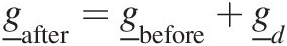
This sediment then needs to be distributed down the profile. Because this sediment is an addition to the profile, the soil profile will become deeper:
 (7.54)
where the definitions of mi are the same as that used for Equation (7.48). The diagonal and off-diagonal terms repeat all the way to the bottom corner (i.e. bottom layer) of the matrix because the deposition pushes down the material in all layers by an amount equal to the mass of deposition. The second term in the equation in  simply ensures that all the deposited material goes into the top layer and nowhere else during that timestep. The similarity with the erosion equation in Equation (7.17) should be clear.
The preceding discussion makes no assumptions about the process driver of deposition. Classically it is sediment being deposited out of fluvial transport. It could also be from aeolian transport (Cohen et al., Reference Cohen, Svoray, Sela, Hancock and Willgoose2015). In this case (aeolian) deposition and fluvial (erosion) can be occurring simultaneously. Cohen showed that if the aeolian material is very fine it can enhance erosion and destroy the armour that might have formed in the absence of aeolian deposition. No matter what the grading of the aeolian material is, it changes the characteristics of the armour layer and potentially changes the fluvial erosion characteristics of the surface.
7.5 Differentiating between Mineral Components
The discussion above has been about differentiating the behaviour of the different fractions within the soil solely on the basis of size. However, the state-space matrix approach can be easily extended to include differentiation based on some other property of the soil. The example we will use here is mineral fractions (e.g. quartz, k-feldspar, biotite etc.), but it will become clear that the techniques outlined below are suitable for labelling any characteristic of the soil (e.g. particle density), or for explicitly modelling nonmineral fractions (e.g. particulate organic matter). Finally the terminology of referring to the  state vector as the grading vector, while convenient so far, will become a bit misleading because the state vector will now contain other, additional, information about the soil, so we will adopt terminology used in the state-space literature and hereafter refer to the grading vector
  as the soil state vector.
In the previous sections the soil state vector  contains the mass of material in each size range without regard to what the characteristics of that material are other than its size. Consider the case where we have three different minerals in the soil that we wish to distinguish (e.g. perhaps they weather at different rates and we would like to track the effect of these different weathering rates on the soil grading as it evolves). Let’s call these minerals Q, K and B to distinguish them. We can then extend our definition of
  so that it now gives the mass in each size range for each of the three minerals for each layer in the soil profile. The vector will then be
(7.55)so that using m size fractions the vector will be 3m in dimension. The horizontal dotted lines in the vector of Equation (7.55) are added simply to highlight the organisation of the vector with the grading of the first mineral first, the second mineral second and the third mineral last. Thus the full  vector is split into three parts with the first third being the
  grading vector for the Q mineral,
  the grading vector for the K mineral and
  the grading vector for the B mineral. This organisation first by mineral and then by grading will be convenient shortly. The A matrix will also be correspondingly bigger and will be of dimension 3m × 3m. While the vector and matrix are larger, the formulation of the A matrix is no more difficult than it was for the nonmineral case. For physical weathering there is no transfer of mass between the mineral fractions, so each mineral fraction is mass conservative in its own right, and then for each mineral fraction we can write the weathering transition matrices
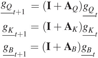 (7.56)
where the A matrices are the matrices that would apply for that mineral if that mineral was 100% of the mass content of the soil layer. We can then write the matrix equation for the full soil state vector for a single soil layer
 (7.57)
The zero off-diagonal matrices indicate that none of the mineral fractions transform into a different mineral fraction during weathering. For physical weathering that is the expected behaviour, but for chemical weathering this may not be the case. If, for instance, one of the mineral fractions is a chemical weathering product of another fraction, then there will be off-diagonal matrices that parameterise the rate and grading characteristics of that weathering process. We can show how this would work in principle by extending our example in Equation (7.57). Imagine that mineral component Q is a weathering product of mineral K, then it is possible to write a matrix equation relating the effect of weather from K to Q on the grading of both Q (the destination of the chemical weathering) and K (the source for the chemical weathering) so that
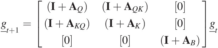 (7.58)
where the transition matrix  calculates how much of mineral K is transformed into mineral Q, what the grading of the source material K was and how it is transformed into the grading of the destination mineral Q, while
  calculates the inverse of how K is transformed into chemical weathering product Q. In general this chemical weathering transformation will not be mass conservative with respect to the soil components because the chemical reactions will typically involve constituents and reactions that have not been tracked in the matrix equations such as hydration (i.e. with water), oxidation (i.e. with oxygen) and carbonation (i.e. with carbon dioxide). All these reactions will change the mass of the soil mineral constituents and can be accounted for with
  ,
,  and
and  . We will focus on chemical weathering in detail in the next chapter (Chapter 8).
In a model for the evolution of organic matter within soils Kirkby (Reference Kirkby1977) proposed a similar method using matrices to differentiate the organic fractions (carbohydrates, amino acids and lignins) and mathematically described how they transformed from one fraction to another. He also proposed a specific structure for the transition matrices for the different types of soil humus, organic sourcing from leaf fall, and examined what the long-term equilibrium organic content of the soil was.
Finally, we note that this section has focussed on the weathering process and differences in weathering rates, but this approach can also be taken with erosion and armouring processes. For instance, it is common for agricultural erosion models to distinguish sediment classes based on their relative transportability (e.g. CREAMS, WEPP; Knisel, Reference Knisel1980; Laflen et al., Reference Laflen, Lane and Foster1991). This transportability is a function of the diameter of the particles and their specific gravity, so these erosion models are potentially capable of distinguishing erosion rates for high specific gravity particles (e.g. high in iron) from midrange specific gravity (e.g. silicates), and low specific gravity particles (e.g. organic matter and soil aggregates).
7.6 The Evolution of Porosity
The layers in the matrix model described above are defined based on the mass per unit area in the layer. To convert these masses per unit area to a depth of soil we need to use the bulk density of the soil in that layer. If the density of particles doesn’t change, then this is equal to the change in the porosity. The main drivers of changes in the density of particles are chemical weathering and the amount of soil carbon. In general the porosity of the soil will change over time simply from the change in the grading and the particle-packing arrangement that is possible with that grading. But porosity will also change with macropore development and changing mineral constituency. If either of these latter properties is being tracked, then these effects can be modelled. For instance, the bioturbation by ants discussed above involves the removal of fine materials from a layer leaving behind voids between the large particles, and will accordingly increase the porosity of the layer from which material is being removed. Note that by defining the soil state vector by mass, this porosity change does not appear in the matrix equations, and appears only at the end when a conversion from mass of soil to depth of soil is required.
For a granular media with two size particles (e.g. a binary media) a relationship due to Fraser (Reference Fraser1935) and Clarke (Reference Clarke1979) based on the percentage of the two sizes is commonly used. This equation has been used (e.g. Morin, Reference Morin2005) and studied by a number of subsequent researchers (Zhang et al., Reference Zhang, Ward and Keller2009). For a granular media made up of a range of particle sizes, a number of empirical extensions of this model (see a comparison by Tranter et al., Reference Tranter, Minasny, McBratney, Murphy, McKenzie, Grundy and Brough2007) can be used to estimate the porosity, ϕ, including (Koltermann and Gorelick, Reference Koltermann and Gorelick1995)
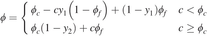 (7.59)
where
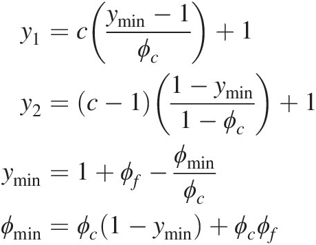 (7.60)
which is applicable for gradings where there are two distinctly different size fractions (e.g. sand/clay, gravel/clay) where ϕf and ϕc are the porosities of the fine and coarse fraction, respectively, and c is the volume fraction of fines. Koltermann and Gorelick showed that this equation fit data better than the ‘perfect packing’ model (Clarke, Reference Clarke1979).
The Koltermann and Gorelick model is only for unstructured granular material and does not account for soil structure effects and organic matter. Tranter et al. (Reference Tranter, Minasny, McBratney, Murphy, McKenzie, Grundy and Brough2007) compared a number of empirical equations for the fraction of the soil smaller than 2 mm (i.e. sand and finer) and found the best fit for the bulk density of the mineral fraction of the soil was
where ps is the percentage of sand by mass, depth is the distance below the soil surface in metres and ρb is in units of g/cm3 or T/m3. To allow for organic matter in the profile it was found sufficient to adjust for its mass fraction (Stewart et al., Reference Stewart, Adams and Abdulla1970)
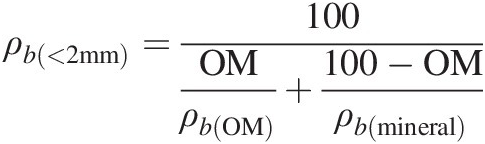 (7.62)
where OM is the percentage of organic matter by mass, and where Tranter used a bulk density of organic matter of 0.224 g/cm3. Finally, Vanwalleghem et al. (Reference Vanwalleghem, Saito, Hayakawa and Oguchi2013) extended this to include the rock fraction (i.e. particles greater than 2 mm) by (Vincent and Chadwick, Reference Vincent and Chadwick1994)
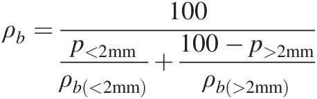 (7.63)
Tranter noted that the root mean square errors of both Equation (7.61), and Equations (7.61) and (7.62) combined, was about 0.15–0.18 g/cm3, or about 10–15%.
However, we still find issues specifically related to the soil history and weathering process that are neglected:
While the Tranter comparison examined soils with significant soil structure, none of the equations in this section explicitly allow for the effect of soil structure (as a result of either clay or organic matter content) on bulk density. Tranter et al. recognised that as a major limitation, but noted that soil grading alone was probably not enough to do better.
The transformation from the native rock in the saprolite, which is by and large unfragmented, to the fragmented rock fragments that result from physical weathering will lead to a decrease in bulk density. This bulk density increase will be reflected in an increase in the porosity. Thus if the fragmented rock particles from physical weathering have a porosity of 0.3 and the saprolite has a porosity of 0.0, then the bulk density will decrease by 30%, and the volume of the space consumed by these rock fragments will increase by 43% after fragmentation.
The rock fragments themselves may change in their density. Chemical weathering may eat away at the inside of the rock fragments without changing the exterior geometry of the particles. This will reduce the bulk density of the soil layer because there is no change in the volume occupied by the particle consumed. Thus there will be no change in the volume of the layer even if there is a change in the mass within that layer. If, however, chemical weathering removes only the outermost rinds of the particles so that the particles get smaller and the soil particles can rearrange themselves to adjust to this change in sizing, then the only change in bulk density will be that given by Equation (7.59) (i.e. only reflecting any change in the grading of the soil). These cases will be discussed in detail in Chapter 8 when chemical weathering is discussed.
At one field site Anderson et al. (Reference Anderson2002) found the bulk density of the soil at the base of the soil profile decreased by more than 50% relative to the parent rock, and ascribed the cause to be a variety of physical weathering and bioturbation (e.g. tree throw) mechanisms. They also performed a chemical mass balance and concluded that an upper bound on the dissolution of minerals could account for only a maximum of a 5% decrease in bulk density. At this site they concluded that the effect of chemical weathering on bulk density is small.
Finally, in an interesting observation Brimhall et al. (Reference Brimhall, Chadwick, Lewis, Compston, Williams, Danti, Dietrich, Power, Hendricks and Bratt1992) noted the possibility that macropores generated by biological activity may fill with deposited material in the long term. They mention tree roots and speculate that after the decay of the roots the empty macropore may fill with mineral or organic matter. Likewise ant and termite galleries might not collapse (and thus might not return the soil bulk density to near its pre-bioturbation value) but may fill up with sediment instead. It is certainly clear that macropores are significant preferential pathways for water flow in the soil (Beven and Germann, Reference Beven and Germann1982, Reference Beven and Germann2013), and it seems reasonable to suggest they would also carry sediment that could fill the macropore in the long term.
7.7 Numerical Issues
Most models break the soil into a series of layers as discussed above. Many of them fix the thickness of, or mass in, the layers. With the exception of mARM, most do not do anything special with the uppermost layer. They simply consider that erosion is a loss of material from the top layer and don’t model the change in the grading that results in armouring. MILESD (Vanwalleghem et al., Reference Vanwalleghem, Saito, Hayakawa and Oguchi2013) uses a different vertical discretisation for the layers, modelling just three layers, corresponding to soil horizons, and models the evolution of the thickness and internal characteristics of these layers. This has the advantage of allowing them to specialise the physics and chemistry to what happens in each of the horizons, but has the disadvantage of not allowing them to investigate what in the physics and chemistry quantitatively drives the development of the horizons in the first place. Subsequently, Temme et al. (Reference Temme and Vanwalleghem2016) implements a series of processes that have no regard for the layers themselves but only the depth of the layers below the surface.
The main numerical issue is the coupling of the surface layer in the physical model with the erosion mechanics. A key feature of the surface is that if there is a coarse weathering-resistant component of the soil, then a surface armour will be formed. This armour consists of the material that cannot be moved by the overland flow, and its existence reduces the erosion rate. Typical armour layer depths in the field are of the order of 1–2 times the diameter of the armour layer, so it is quite thin relative to the depth of the soil. Thus we have found that you need a thin surface layer to correctly capture the armouring process. Thicker layers then underlie this, so that there aren’t an unnecessarily large number of layers within the profile.
In the existing models of physical weathering some have defined the layers based on thickness of the layer, while others have defined them on the basis of mass within the layer. The mARM model defined the layers on thickness, but we have subsequently found that this definition makes formulation of the transition matrices complex, particularly if the layers are different thickness, so we advise using mass as the definition of the layer. This means that you need to have a model for porosity so that this mass can be converted to soil depth, but this is implicit in the soil thickness formulations.
A related issue is how to define the size fractions within the layer. In mARM we defined them on the basis of the proportion by mass within each size fraction. This is consistent with how particle size distributions are normally expressed in the soil science community. However, subsequent experience has been that formulation using the mass (rather than proportion) in each size within each layer is computationally and conceptually easier, and consistent with the mass per layer formulation.
Defining each layer by mass avoids another issue, which is whether to define the layer boundaries by (1) elevations relative to the soil surface (which itself is changing as a result of the erosion and landform evolution) or (2) absolute elevations (e.g. above sea level). Defining the layers with mass avoids the need to define the elevation of the boundaries in the soil model except when weathering rates need to be determined relative to the surface, in which cases all layers are relative to the evolving soil surface.
If porosity is changing, then the thickness of each layer will naturally change relative to how much mass is in each layer. It is then conceivable that the soil surface elevation will rise if the right combination of changes in porosity and mass within all the layers occurs. For instance, consider the case of the dilation of a soil due to tree throw, but where erosion is low. The porosity increase as a result of the tearing out of the saprolite of the rock will inevitably lead to a soil thickening and a rise in elevation of the soil surface.


