


I. INTRODUCTION
Airborne synthetic aperture radar (SAR) systems are capable of high-resolution imaging of earth surfaces that is required in many practical applications. The quality of SAR images essentially depends on the precision of the aircraft trajectory measurements [Reference Oliver and Quegan1–Reference Carrara, Goodman and Majewski3]. Uncompensated motion errors cause range delays and phase errors in the received radar data resulting in distortions of SAR images. However, the accurately measured deviations of the trajectory from the reference straight line can be compensated [Reference Franceschetti and Lanari2–Reference Bezvesilniy and Vavriv5] with minor deteriorations of image quality. The problem is that in the case of a very high resolution and/or a light-weight aircraft platform, even expensive navigation systems do not guarantee the required accuracy of measurements. For such situations, autofocus methods have been developed for precise estimation of the motion errors directly from the received radar data [Reference Oliver and Quegan1–Reference Cumming and Wong4].
Autofocus techniques can be divided into two general classes – parametric and nonparametric. The parametric autofocus methods use some model for the platform motion. The aim of the methods is to estimate the parameters of the model. The map-drift autofocus (MDA) [Reference Oliver and Quegan1, Reference Carrara, Goodman and Majewski3, Reference Li, Held, Curlander and Wu6–Reference Samczynski and Kulpa9] is a widely known parametric method. It estimates the quadratic phase error in the data by measuring the linear shift between two SAR images built by dividing the azimuth processing interval on two halves. The multiple-aperture MDA [Reference Carrara, Goodman and Majewski3, Reference Calloway and Donohoe10] estimates the phase error as a higher-order polynomial. Other models, such as a Fourier series, have also been proposed [Reference Calloway and Donohoe10–Reference Cantalloube and Nahum12]. The problem is that the parametric autofocus methods are restricted by the models applied.
The nonparametric methods do not use approximation models for phase errors. One of the most powerful nonparametric methods is the phase gradient autofocus (PGA) [Reference Carrara, Goodman and Majewski3, Reference Wahl, Eichel, Ghiglia and Jakowatz13, Reference Wahl, Jakowatz, Thompson and Ghiglia14]. It estimates the first derivative (the gradient) of the azimuth phase error function from signals backscattered from isolated point targets. However, the PGA is intended mainly for the spotlight SAR mode. In this SAR mode, the signal from every point target on the scene is presented in each radar pulse, and the phase error is almost independent on range. In the strip-map SAR mode, the application of the PGA method is complicated because the target echoes are presented in the data only during the time required for the target to cross the antenna beam. It means that the signal of each selected point target contains only a small part of the complete phase error function. Moreover, in the strip-map mode, the range dependence of the phase errors can be significant and should be taken into account when averaging the autofocus estimates across the swath.
In this paper, a new approach to the strip-map SAR autofocus is presented. The method is called the local-quadratic MDA (LQMDA). The idea of the method is to estimate the local quadratic phase errors on short azimuth intervals. Such estimates are performed independently for a number of range blocks across the swath. Using the range dependence of the phase errors, the uncompensated cross-track components of the aircraft acceleration are evaluated for each short azimuth time interval. Finally, the residual trajectory deviations are obtained by double integration of the estimated acceleration. The proposed method is non-parametric allowing the estimation of an arbitrary smooth range-dependent phase error function. The LQMDA method has similarities with the reflectivity displacement method [Reference Moreira15–Reference Buckreuss17]. Both methods use local estimates of the motion errors and the integration steps to evaluate the phase error function.
The proposed LQMDA method does not require the presence of bright points on the scene and can be used both in the strip-map and spotlight SAR modes. This method refines the aircraft trajectory to a high precision so that high-quality multi-look SAR images can be produced. The developed autofocus technique has been successfully tested on practice using radar data obtained with the X-band airborne SAR system [Reference Bezvesilniy and Vavriv5, Reference Vavriv18]. Main characteristics of the SAR system are listed in Table 1. Some early results on the LQMDA technique have already been published [Reference Gorovyi, Bezvesilniy and Vavriv19] and presented in several conferences [Reference Bezvesilniy, Gorovyi and Vavriv20–Reference Gorovyi, Bezvesilniy and Vavriv24].
Table 1. Main characteristics of the RIAN-SAR-X system.

The paper is organized as follows. In the next section, the frame-based SAR processing and common motion error compensation (MOCO) procedures are discussed. Section III describes the developed LQMDA in detail, including the incorporation of the method within the framework of the range-Doppler algorithm (RDA). Experimental results are presented and discussed in Section IV, and a brief conclusion is given in Section V.
II. FRAME-BASED SAR PROCESSING AND MOCO
The SAR data processing is commonly organized on a frame-by-frame basis; each data frame counts many intervals of synthesis. A scheme with half-overlapped frames is illustrated in Fig. 1. In such scheme, each backscattered pulse is put in two frames, and these two frames are processed independently and simultaneously, in parallel, in the hardware. Each frame is processed with its own reference straight flight trajectory, the reference aircraft flight altitude, velocity, and orientation. The SAR images obtained from the sequence of data frames are then stitched together to form a longer strip-map SAR image.

Fig. 1. SAR processing with half-overlapped data frames.
The SAR image of each frame has invalid zones at its azimuth edges, where the image brightness decays to zero. This is because these areas of the scene are only partly illuminated by the antenna beam during the data frame acquisition time. Neighbor frames have significant overlapped areas. It helps image stitching and guarantees continuous surveillance of the strip without gaps despite of possible motion instabilities.
Due to the frame-based processing, the trajectory deviations and orientation errors are kept relatively small within the frame, and many approximate algorithms for MOCO can be used.
The navigation system of the airborne RIAN-SAR-X system [Reference Bezvesilniy and Vavriv5, Reference Vavriv18] is designed as follows. The hardware part of the navigation system is based on a simple global positioning system receiver capable of measuring the aircraft position and velocity. The position is measured with accuracy of an order of several meters and used to link the obtained SAR images to ground maps and also to get the flight altitude above the ground. The accuracy of the velocity measurements is as high as 0.05 m/s.
The accurate aircraft flight trajectory is integrated from the measured aircraft velocity to perform MOCO in real time. The achieved accuracy is sufficient to produce full-resolution (up to 2 m) SAR images (X-band) with up to 15 looks (except some cases of very rough flight conditions). Later, at the data post-processing stage, the aircraft trajectory is further refined by using an autofocusing method described in this paper that allows processing the full Doppler bandwidth and forming high-quality SAR images with up to 35 looks at 2 m resolution.
The antenna beam orientation in the RIAN-SAR-X system is evaluated from the measured Doppler frequency of the backscattered radar signals in real time [Reference Bezvesilniy and Vavriv5]. With such technique, the angles are determined with respect to the current aircraft velocity vector (regardless of the orientation of the aircraft construction axes). The estimated pitch and yaw angles are averaged during the data frame acquisition time and used as the reference angles both for motion compensation and for aperture synthesis. Due to the averaging, the reference angles are assumed to be defined with respect to the reference flight line. Such angle estimation is a kind of clutter-lock processing allowing us to adjust our SAR data processing algorithms for each data frame in real time to track variations of the antenna beam orientation and avoid significant radiometric errors. The variations of the antenna pitch and yaw angles within the data frame caused by the aircraft orientation errors, as well as the aircraft drift and flight direction deviation effects are ignored in real time, but can be compensated via the multi-look radiometric correction with extended number of looks [Reference Bezvesilniy and Vavriv5] at the post-processing stage if necessary.
The MOCO procedure typically includes data interpolation and phase correction steps. The along-track trajectory errors are equivalent to non-uniform spatial sampling of the data. These errors can be compensated by data interpolation in the azimuth direction. Alternatively, the pulse repetition frequency (PRF) can be adjusted from pulse to pulse according to the current aircraft velocity in order to keep the inter-pulse aircraft path constant. The first approach was implemented in the airborne RIAN-SAR-X system and the second one in the RIAN-SAR-Ku system [Reference Bezvesilniy and Vavriv5].
The along-track error compensation is followed by the slant range (or the line-of-sight) error correction. The geometry of the motion compensation problem is illustrated in Fig. 2. The point A (0, 0, H) indicates the expected position of the aircraft on the reference straight line trajectory. The local coordinate system (x, y, z) is sliding along the data frame coordinate system (X, Y, Z). The point A
E
(Δx
E
, Δy
E
, H + Δz
E
) corresponds to the actual position on the real trajectory; the vector ${{\bf \vec r}_E} = \left( {\Delta {x_E},\;\Delta {y_E},\;\Delta {z_E}} \right)$
describes trajectory deviations. Despite the along-track error compensation by interpolation, some small along-track errors Δx
E
can still be presented.
${{\bf \vec r}_E} = \left( {\Delta {x_E},\;\Delta {y_E},\;\Delta {z_E}} \right)$
describes trajectory deviations. Despite the along-track error compensation by interpolation, some small along-track errors Δx
E
can still be presented.
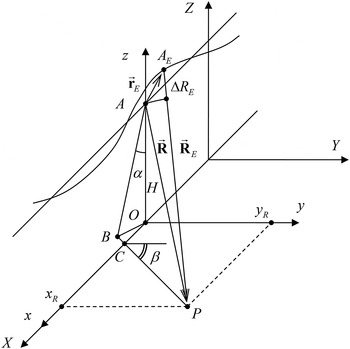
Fig. 2. Slant range MOCO.
The coordinates of the point P(x R , y R , 0) (Fig. 2) located on the Doppler centroid line at range R are
 $${x_R} = H\tan \alpha \cos \beta + \sin \beta \sqrt {{R^2} - {H^2} - {{\left( {H\tan \alpha} \right)}^2}}, $$
 $${y_R} = - H\tan \alpha \sin \beta + \cos \beta \sqrt {{R^2} - {H^2} - {{\left( {H\tan \alpha} \right)}^2}}. $$
Here α and β are the reference antenna beam pitch and yaw angles. The pitch angle α is the angle between the nadir direction AO and the perpendicular line AB plotted to the Doppler centroid line CP, which is the intersection of the ground plane and the elevation plane of the antenna beam pattern. The yaw angle β is the angle between the Doppler centroid line CP and the y-axis.
The slant range error for the synthetic beam directed to the point P(x R , y R , 0) is calculated as
 $$\Delta {R_E}\left( {{x_R},\;{y_R}} \right) = {R_E}\left( {{x_R},\;{y_R}} \right) - R,$$
 $${R_E}\left( {{x_R},\;{y_R}} \right) = \sqrt {{{\left( {\Delta {x_E} - {x_R}} \right)}^2} + {{\left( {\Delta {y_E} - {y_R}} \right)}^2} + {{\left( {H + \Delta {z_E}} \right)}^2}}. $$
The corresponding range migration error is compensated by interpolation in the range direction. The corresponding phase error
 $${\varphi _E}\left( {{x_R},\;{y_R}} \right) = - \displaystyle{{4\pi} \over \lambda} \Delta {R_E}\left( {{x_R},\;{y_R}} \right)$$
is compensated by complex conjugate multiplication.
The motion error correction should not interfere with the range and azimuth compressions. Any range-dependent motion compensation cannot be applied before the range compression (RC) of the received radar pulses. Otherwise, the range linear frequency modulation (LFM) waveform of the radar pulses will be distorted. Moreover, the range-dependent compensation cannot be applied before the range migration correction step of the SAR processing algorithm. Otherwise, different corrections applied for the neighbor range bins will introduce phase errors in the azimuth direction after the range migration correction.
To cope with the above problems, the motion compensation procedure for the range-Doppler algorithm (and similar fast Fourier transform (FFT)-based algorithms) [Reference Bezvesilniy and Vavriv5] is usually divided into two steps [Reference Franceschetti and Lanari2]:
-
1. First-order range-independent motion compensation.
-
2. Second-order range-dependent motion compensation.
The first-order motion compensation includes the range delay of the received pulses (with interpolation) and the phase compensation, which are calculated for some reference range, for example, for the center range of the swath R C ,
 $$\phi _E^{(I)} \left( {{R_C},t} \right) = \exp \left[ { - i\displaystyle{{4\pi} \over \lambda} \Delta R_E^{(I)} \left( {{R_C},t} \right)} \right].$$
Here t is the flight time. The first-order motion compensation can be incorporated into the RC step but it should be performed before any processing step in the azimuth, in particular, before the range migration correction in the range–Doppler algorithm.
The second-order range-dependent motion compensation is performed after the RC and the range migration correction steps,
 $$\Delta R_E^{(II)} \left( {R,\;t} \right) = \Delta {R_E}\left( {R,\;t} \right) - \Delta R_E^{(I)} \left( {{R_C},\;t} \right),$$
 $$\phi _E^{(II)} \left( {R,\;t} \right) = \exp \left[ { - i\displaystyle{{4\pi} \over \lambda} \Delta R_E^{(II)} \left( {R,\;t} \right)} \right].$$
It includes the phase compensation and may include the range interpolation if necessary.
Since the motion errors depend on time, the data after the range migration correction should be transformed from the range-Doppler domain back to the time domain to apply the second-order motion error correction and then again to the range-Doppler domain to perform the azimuth compression.
After the MOCO, the data seem to be collected from the reference straight line trajectory, and the range-Doppler processing is performed by using the reference parameters of the data frame.
III. LOCAL-QUADRATIC MAP-DRIFT AUTOFOCUS
In this paper, an efficient autofocusing technique is described for the estimation of the residual trajectory deviations directly from the SAR data. The method is called the LQMDA. The idea of the method consists of estimating the local quadratic phase errors on small time intervals using the well-known map-drift principle [Reference Franceschetti and Lanari2, Reference Cumming and Wong4]. It has been shown that the local quadratic phase errors are related to the cross-track components of the aircraft acceleration. The range dependence of the phase errors is essentially used in the algorithm to resolve the vertical and horizontal acceleration components. The uncompensated trajectory deviations for the whole data frame are then derived by double integration of the evaluated acceleration. Below, the LQMDA method is described in detail.
The SAR image formed from the data collected on a short time interval shows the part of the scene illuminated by the real antenna beam during this short time. For autofocusing, the duration of the short time intervals T S is assumed to be much smaller than the time required for the target to cross the real antenna footprint. In this case, the illuminated part of the scene is approximately equal to the antenna footprint area. For example, for the azimuth antenna beam width θ A = 10°, the antenna footprint on the ground at a slant range R = 4 km is L A ≈ Rθ A ≈ 700 m. The synthetic aperture length required to achieve a moderate azimuth resolution ρ = 3 m is only L S ≈ K w λR/(2ρ) ≈ 26 m (for λ = 3 cm and the weighting window coefficient K w = 1.3) that is indeed a small fraction of the antenna footprint size.
Assuming that the intervals are short enough, the residual phase error function within each interval can be approximated by the second-order polynomial:
 $$\eqalign{{\phi _E}\left( {R,\;{t_n} + \tau} \right) \approx {\phi _E}\left( {R,\;{t_n}} \right) + {\phi ^{\prime}_E}\left( {R,\;{t_n}} \right)\tau + {\phi ^{\prime \prime}_E}\left( {R,\;{t_n}} \right){\tau ^2}/2.}$$
The variable τ represents the time within the short interval − T S /2 <τ <T S /2. The described local representation can be efficiently used for the estimation of an arbitrary residual phase error function. We propose to estimate the local quadratic phase error coefficients φ″ E (R, t n ) on each short interval separately by using the map-drift principle. According to this autofocus technique, the short processing interval is divided into two parts, and two SAR images are built. The presence of the quadratic error shifts the images in the azimuth in the opposite directions by Δt max = Δx max /V, V is the aircraft velocity. The shift can be measured from the position of the maximum of the correlation function of two images. The local quadratic phase error coefficient is given by
 $${\phi ^{\prime \prime}_E}\left( {R,\;{t_n}} \right) = 2\pi F_{DR}^E \left( {R,\;{t_n}} \right) = 2\pi {F_{DR}}(R)\Delta {t_{max}}/\left( {{T_S}/2} \right),$$
where F DR is the Doppler rate of the SAR matched filter.
Thus, by using the map-drift principle, the local quadratic phase error coefficient φ″ E (R, t n ) can be estimated. The constant term φ E (R, t n ) does not affect the estimation and can be omitted, as well as the linear term φ′ E (R, t n )τ that only shifts the two SAR images in the azimuth in the same direction. So, we can estimate the samples of the second derivative of the error function and then reconstruct the error function by double integration.
On the one hand, the length of the short intervals should be chosen to provide a sufficient precision of the parabolic phase error approximation. On the other hand, the length should be increased iteratively up to the length of synthesis required to achieve the desired high azimuth resolution on the final SAR image.
In order to reduce the number of computations, the dechirp method [Reference Carrara, Goodman and Majewski3, Reference Cumming and Wong4] can be used for the SAR image formation on the short time intervals. According to this technique, the pair of images can be obtained as follows:
 $${I_1}(f) = \displaystyle{2 \over {{T_S}}}\int_{ - {T_S}/2}^0 {{w_S}\left( {\tau + {T_S}/4} \right)s(\tau ){h^*}(\tau )\exp [ - 2\pi if\tau ]d\tau}, $$
 $${I_2}(f) = \displaystyle{2 \over {{T_S}}}\int_0^{{T_S}/2} {{w_S}\left( {\tau - {T_S}/4} \right)s(\tau ){h^*}(\tau )\exp [ - 2\pi if\tau ]d\tau}. $$
Here w S (τ) is the weighting window. The reference function h(t) is given by
 $$h(t) = \exp \left[ {2\pi i\left( {{F_{DC}}t + {F_{DR}}{t^2}/2} \right)} \right],$$
where F DC and F DR are the known Doppler centroid and Doppler rate. The spatial frequency f is related to the azimuth time as f = F DR t. Due to the dechirp processing (11) and (12), one can form the SAR image from each half-interval by using a single short Fourier transform.
In the presence of a local quadratic phase error, the SAR images will be defocused and shifted in the azimuth in the opposite directions. The shift is described by the following equation:
 $$\Delta {f_{max}} = {f_{1max}} - {f_{2max}} = F_{DR}^E {T_S}/2.$$
The common way to measure the shift is to calculate the cross-correlation function of the pair of SAR images. For a particular range gate, it is determined as
 $${R_{CC}}(R,\Delta f) = \int {{{\left \vert {{I_1}\left( {R,f} \right)} \right \vert} ^2}{{\left \vert {{I_2}\left( {R,f + \Delta f} \right)} \right \vert} ^2}df}. $$
One should note that the efficiency of such measurement significantly depends on the images content. In particular, the low image contrast can lead to inaccurate estimation of the peak position. In order to improve the estimation quality, several pre-processing steps should be performed. At first, the images are recalculated into a logarithmic scale and the dynamic range is narrowed. It allows balancing the contributions from bright and dark image features. After that, the local centering is performed, enhancing the local contrast of image details and significantly narrowing the correlation peaks. The image pre-processing significantly improves the precision of the peak position estimation.
The problem is that the motion errors in the data are range dependent. It means that the phase error functions have to be estimated for each range gate. In order to take into account the range dependence, we propose to estimate the cross-track components of the aircraft acceleration, a Y (t n ) and a Z (t n ), which are responsible for the local quadratic phase errors and related to the estimated values φ″ E (R, t n ). We expect that the along-track component of the acceleration is measured by the SAR navigation system more accurately than the cross-track components. Therefore, the residual (uncompensated) along-track acceleration a X (t n ) is assumed to be negligibly small compared with the cross-track ones. The details of the approach are as follows.
Let us approximate the aircraft trajectory on a short time interval as
 $${{\bf \vec r}_A}\left( {{t_n},\tau} \right) = {\bf \vec H} + {\bf \vec V}\left( {{t_n}} \right)\tau + {{\bf \vec r}_E}\left( {{t_n},\tau} \right),$$
 $${{\bf \vec r}_E}\left( {{t_n},\tau} \right) \approx {\bf \vec r}\left( {{t_n}} \right) + {\bf \vec v}\left( {{t_n}} \right)\left( {{t_n} + \tau} \right) + {\bf \vec a}\left( {{t_n}} \right){\left( {{t_n} + \tau} \right)^2}/2\;.$$
Here ${{\bf \vec r}_E}({t_n},\tau )$
represents the residual trajectory deviations;
${{\bf \vec r}_E}({t_n},\tau )$
represents the residual trajectory deviations; ${\bf \vec H} = (0,\;0,\;H)$
and
${\bf \vec H} = (0,\;0,\;H)$
and ${\bf \vec V} = (V,\;0,\;0)$
are the reference flight altitude and velocity vectors. The Doppler rate of the backscattered signal under such motion, assuming that
${\bf \vec V} = (V,\;0,\;0)$
are the reference flight altitude and velocity vectors. The Doppler rate of the backscattered signal under such motion, assuming that $\left\vert {{{{\bf \vec r}}_E}({t_n})} \right\vert \; \ll R$
, is
$\left\vert {{{{\bf \vec r}}_E}({t_n})} \right\vert \; \ll R$
, is
 $$\eqalign{& {F_{DR}}\left( {R,\;{t_n}} \right) \approx \cr & \quad - \displaystyle{2 \over \lambda} \left[ {\displaystyle{1 \over R}\left( { \vert {\bf \vec V} + {\bf \vec v}({t_n}){ \vert ^2} - {{\left( {\displaystyle{{{\bf \vec R} \cdot \left( {{\bf \vec V} + {\bf \vec v}\left( {{t_n}} \right)} \right)} \over R}} \right)}^2}} \right) - \displaystyle{{{\bf \vec R} \cdot {\bf \vec a}\left( {{t_n}} \right)} \over R}} \right],} $$
where ${\bf \vec R} = ({x_R},\;{y_R}, - H)$
is the slant range vector.
${\bf \vec R} = ({x_R},\;{y_R}, - H)$
is the slant range vector.
The estimated local quadratic phase errors are related to the Doppler rate errors. The main contribution to these errors is introduced by the uncompensated cross-track acceleration:
 $$F_{DR}^E \left( {R,\;{t_n}} \right) \approx \displaystyle{2 \over \lambda} \displaystyle{{{\bf \vec R} \cdot {\bf \vec a}\left( {{t_n}} \right)} \over R} \approx \displaystyle{2 \over \lambda} \displaystyle{{{y_R}{a_Y}\left( {{t_n}} \right) - H{a_Z}\left( {{t_n}} \right)} \over R}.$$
The uncompensated velocity ${\bf \vec v}({t_n})$
has a minor influence; it is accounted implicitly during iterations of the autofocus procedure. From the above formula one can easily write a system of linear equations that provide the mean-square-error (MSE) estimates for the acceleration components:
${\bf \vec v}({t_n})$
has a minor influence; it is accounted implicitly during iterations of the autofocus procedure. From the above formula one can easily write a system of linear equations that provide the mean-square-error (MSE) estimates for the acceleration components:
 $$\eqalign{& MSE\left( {{a_Y}\left( {{t_n}} \right),{a_Z}\left( {{t_n}} \right)} \right) = \cr & \quad \sum\limits_{m = 1}^{{M_R}} {{w_m}{{\left[ {\displaystyle{2 \over \lambda} \displaystyle{{{y_{{R_m}}}{a_Y}\left( {{t_n}} \right) - H{a_Z}\left( {{t_n}} \right)} \over {{R_m}}} - F_{DR}^E \left( {{R_m},{t_n}} \right)} \right]}^2}},} $$
where w m are weighting coefficients which are determined as the values of the cross-correlation functions maxima. Such choice can be justified. The value of the cross-correlation peak is proportional to the image contrast. The higher the contrast of the range block the better is the estimation precision, and vice versa. Therefore, such weighting improves the overall performance of the MSE scheme and leads to a more precise cross-track acceleration evaluation.
The MSE estimator equations are
 $$\eqalign{& {a_Y}\left( {{t_n}} \right)\sum\limits_{m = 1}^{{M_R}} {{w_m}{{\left( {\displaystyle{{{y_{{R_m}}}} \over {{R_m}}}} \right)}^2} -} \,{a_Z}\left( {{t_n}} \right)\sum\limits_{m = 1}^{{M_R}} {{w_m}\left( {\displaystyle{{{y_{{R_m}}}} \over {{R_m}}}\displaystyle{H \over {{R_m}}}} \right)} = \cr & \quad \displaystyle{\lambda \over 2}\sum\limits_{m = 1}^{{M_R}} {{w_m}F_{DR}^E \left( {{R_m},{t_n}} \right)} \displaystyle{{{y_{{R_m}}}} \over {{R_m}}},} $$
 $$\eqalign{& {a_Y}({t_n})\sum\limits_{m = 1}^{{M_R}} {{w_m}\left( {\displaystyle{{{y_{{R_m}}}} \over {{R_m}}}\displaystyle{H \over {{R_m}}}} \right) - } {a_Z}\left( {{t_n}} \right)\sum\limits_{m = 1}^{{M_R}} {{w_m}{{\left( {\displaystyle{H \over {{R_m}}}} \right)}^2}} = \cr & \quad \displaystyle{\lambda \over 2}\sum\limits_{m = 1}^{{M_R}} {{w_m}F_{DR}^E \left( {{R_m},{t_n}} \right)} \displaystyle{H \over {{R_m}}}.} $$
By solving this system independently for each short time interval with the center at t n , the sequence of the estimated acceleration a Y (t n ), a Z (t n ) is obtained. The residual trajectory deviations are calculated by double integration and used for the motion compensation.
The LQMDA technique can be easily incorporated into the conventional SAR processing algorithm such as the RDA, as illustrated in Fig. 3. At first, the received raw data are compressed in range and the first-order range-independent motion compensation is applied. The range-compressed data can be pre-filtered and decimated in the azimuth direction from a high PRF to a lower azimuth sampling frequency that corresponds to the Doppler bandwidth determined by the antenna beam width. Then, the range cell migration correction (RCMC) is performed in the range-Doppler domain. After that, the second-order range-dependent motion compensation is accomplished. For the first time, the motion compensation steps are based on the flight trajectory measured by the SAR navigation system. After these steps, the data is ready for the application of the LQMDA, which is intended to estimate the residual trajectory deviations.

Fig. 3. LQMDA incorporated within the framework of the range–Doppler algorithm.
The main steps of the LQMDA algorithm are illustrated in Fig. 4. The whole data frame after RC and RCMC is divided on short data blocks in the azimuth direction. Each data block is split into two halves and two SAR images for the MDA estimation are formed using the dechirp-based processing (11) and (12). From the image shifts (15), the local quadratic phase errors and the corresponding Doppler rate errors (14) are evaluated for each azimuth block for a set of range blocks. By using the described MSE fitting procedure (20)–(22), the cross-track accelerations are estimated. After that, by double integration, the residual trajectory deviations are derived for the whole processed data frame. Finally, the refined aircraft trajectory is accounted by introducing corrections to the first- and second-order MOCO steps (see Fig. 3).

Fig. 4. Steps of the LQMDA.
The described autofocusing procedure should be iterated several times for the best result. With the iterations, the aircraft trajectory is refined, and the motion compensation procedures are repeated, reducing the residual motion errors. Moreover, the length of the short intervals is enlarged (e.g. doubled) iteratively, increasing the resolution of the pair of SAR images and, consequently, improving the accuracy of the MDA estimation.
After the application of the LQMDA technique, the data is ready for the conventional multi-look synthesis in the range-Doppler domain (Fig. 3), producing the well-focused SAR image.
The described LQMDA technique has been realized as a post-processing procedure applied to the recorded SAR data. However, all computations can be efficiently optimized via parallel processing in azimuth, in range, in frequency. Therefore, the real-time implementation of the algorithm might be possible depending on the computation power of the data-processing hardware.
IV. EXPERIMENTAL RESULTS
The developed LQMDA method has been successfully applied to radar data obtained with the airborne RIAN-SAR-X system [Reference Bezvesilniy and Vavriv5, Reference Vavriv18]. A 25-look SAR image with a 2 m resolution built without autofocusing is shown in Fig. 5(a). One can see that the image is significantly defocused. The well-focused SAR image built with the proposed LQMDA algorithm is shown in Fig. 5(b). The image shows significant improvement. One can now recognize lots of fine details, sharp edges, and readable radio-shadows. The provided example demonstrates the high efficiency of the LQMDA method.

Fig. 5. (a). A 25-look 2 m resolution SAR image before autofocusing. (b). A 25-look 2 m resolution SAR image after autofocusing.
The potential of the proposed LQMDA technique has also been demonstrated in the following way. A fragment of the ground scene indicated by a dash line in Figs 5(a) and 5(b) has been rebuilt with a set of different azimuth resolutions of 4, 2, 1, and 0.5 m. The corresponding images are shown in Fig. 6. The number of looks is changed as 49, 25, 13, and 7, respectively, in accordance to the resolution to keep constant the multi-look processing interval. The images are given in the ground plane coordinates: the vertical direction is the ground range and the horizontal direction is the azimuth. The pixel size is 0.25×0.25 m. The ground range resolution is limited to 3 m in these images because of the 2 m slant range resolution of the SAR system. Going from 4 m to 2 m, and then to 1 m, and 0.5 m azimuth resolutions one can distinguish many point-like targets in the images. Two illustrative targets have been selected and labeled as 1 and 2 in Fig. 6. The azimuth profiles of these targets are shown in Figs 7(a) and 7(b), respectively. The peak of the target 1 in Fig. 7(a) becomes narrower for a finer resolution as it is expected for a point target. The target 2 looks like a “point target” at the 4 m resolution, however, it is actually composed of five individual point scatterers as clearly resolved at the 0.5 m resolution, as shown in Fig. 7(b). This demonstration proves that the LQMDA technique does provide the accuracy of the trajectory estimation sufficient to achieve the azimuth resolution up to 0.5 m with seven looks.

Fig. 6. Fragment of the ground scene built with a set of different azimuth resolutions.

Fig. 7. Azimuth profiles of the point-like targets 1 and 2 (Fig. 6) built with a set of different azimuth resolutions of 0.5, 1, 2, and 4 m.
V. CONCLUSION
The efficient LQMDA technique for airborne SAR systems has been developed and tested. The method estimates the cross-track components of the aircraft acceleration locally on short time intervals. After that, the residual trajectory deviations for whole data frame are evaluated by double integration. The high efficiency of the method has been confirmed by processing the airborne SAR data. The method is especially useful for SAR systems operated from light-weight aircrafts.
ACKNOWLEDGEMENTS
The authors thank all their colleagues at the Department of Microwave Electronics of the Institute of Radio Astronomy of the National Academy of Sciences of Ukraine for their efforts in the development of SAR systems.
 Oleksandr O. Bezvesilniy received the Dipl. degree in Radio Physics from the Kharkiv State University, Ukraine in 1999, and received the Ph.D. degree in Radio Physics at the Institute of Radio Astronomy of the National Academy of Sciences of Ukraine in 2007. His research interests include signal and image processing for synthetic aperture radars and for meteorological radars.
 Ievgen M. Gorovyi received the Master degree in Radio Physics from the Kharkiv State University, Kharkiv, Ukraine in 2010 and the Ph.D. degree in Radio Physics from the Institute of Radio Astronomy of the National Academy of Sciences of Ukraine, Kharkiv in 2014. His main research interests include SAR autofocusing, signal and image processing, and computer vision.
 Dmytro M. Vavriv received the Dipl. degree in Radio Physics from the Kharkov State University, Ukraine in 1975, and received the Ph.D. degree in radio physics and the D.Sc. degree in Physics and Mathematics in 1979 and 1988, respectively. Since 1989, he has been the Head of the Department of Microwave Electronics at the Institute of Radio Astronomy of the National Academy of Sciences of Ukraine and a Professor at the Kharkov State University. In 2006, he became a Corresponding Member of the National Academy of Sciences of Ukraine. He has published eight books and book chapters and over 300 papers. His research interests include radar systems, millimeter-wave tubes, signal processing, chaos, and nonlinear phenomena.


