


1. Motivation
Why is it, as empirical evidence suggests, that controlling for men's wealth, the riskiness of the manner in which men manage their finances is linked with their marital status (single, married, and, if married, subject to the likelihood of divorce)? In this paper we propose a causal link. We postulate that the potential for success in one market, here the marriage market, affects incentives in another market that is linked to the marriage market via an individual's relative wealth. Behavior is guided by a desire to obtain a better relative position in terms of wealth distribution, an outcome that, in turn, would lead to a better match in the marriage market. Our idea is that although married men who are not in the marriage market do not or need not worry about their prospects in that market, married men who expect to re-enter that market because of the “background” divorce rates (determined by social, cultural, or legal factors) that they face will worry somewhat. We show how this variation in the association with the marriage market maps onto risk-taking behavior.
Recent empirical research links the likelihood of divorce with risk aversion. A positive correlation between the two has been noted in several studies. For example, analyzing US data from the National Longitudinal Survey of Youth (NLSY79) between 1979 and 2004, Light and Ahn (Reference Light and Ahn2010) find a positive relationship between risk tolerance, as measured by the willingness to accept alternative lifetime income gambles, and a predicted probability of divorce. Roussanov and Savor (Reference Roussanov and Savor2014) report that CEOs of firms that are located in US states in which divorce is less costly for the richer spouse (presumably male CEOs), and hence more likely, are less risk averse than CEOs of firms located in states in which the cost of divorce is higher. These findings prompted us to wonder whether the risk aversion of a married individual might be influenced by his “background” likelihood of divorce and a corresponding likelihood of reentering the marriage market.Footnote 1, Footnote 2
The received literature has long correlated high status with superior outcomes in the marriage market: see Becker (Reference Becker1973) for a theoretical foundation, Cole et al. (Reference Cole, Mailath and Postlewaite1992, Reference Cole, Mailath and Postlewaite2001), Robson (Reference Robson1996), Wei and Zhang (Reference Wei and Zhang2011), and Wei et al. (Reference Wei, Xiaobo and Yin2017), among others, for more recent formulations. Several of these models identify status with relative wealth, in line with a long tradition in economics. Smith (Reference Smith1759) argues that wealth accumulation yields social status, and that status matters for individual welfare. Veblen (Reference Veblen1899) dwells at length on the notion that in modern Western societies the aspiration for high relative wealth is motivated by an underlying desire for social status. In his study of the origins of modern English society, Perkin (Reference Perkin1969, p. 85) comments that “the pursuit of wealth was the pursuit of social status.” Frank (Reference Frank1985) emphasizes the significance of relative wealth for the acquisition of social status. A formal link between social status and individuals’ relative wealth is provided in models developed, among others, by Corneo and Jeanne (Reference Corneo and Jeanne1997), Futagami and Shibata (Reference Futagami and Shibata1998), Pham (Reference Pham2005), and Roussanov (Reference Roussanov2010).Footnote 3
How does a stronger distaste at having a low position in the (domain of) wealth distribution transform into lower risk aversion? This is an important question because, although there are studies that link relative wealth or relative consumption with risk aversion (Campbell and Cochrane, Reference Campbell and Cochrane1999; Gollier, Reference Gollier2004), thus far the behavioral mechanism that underlies the transmission from a well-defined measure of displeasure at having a low position in wealth distribution to a well-defined measure of risk aversion has not been uncovered; it is as if we have an input going into and an output coming out of a black box, but no knowledge of the processing that takes place inside the box.Footnote 4
The preceding discussion prompted a commentary on an earlier version of this paper, to the effect that greater risk aversion will usually lead to less risky gambling, especially among the initially wealthy. However, as demonstrated by Stark (Reference Stark2019), the relationship between a change in wealth and risk aversion is more complex. Stark explores a link between the concern over having low relative wealth, the level of wealth, and risk aversion. Specifically, Stark studies the relative risk aversion of an individual with particular social preferences: his wellbeing is influenced by his relative wealth, and by how concerned he is about having low relative wealth. Holding constant the individual's absolute wealth, two results are obtained. First, if the individual's level of concern about low relative wealth does not change, the individual becomes more risk averse when he rises in the wealth hierarchy. Second, if the individual's level of concern about low relative wealth intensifies when he rises in the wealth hierarchy and if, in a precise sense, this intensification is strong enough, then the individual becomes less risk averse: the individual's desire to advance further in the wealth hierarchy is more important to him than possibly missing out on a better rank.
In sum: what the current paper demonstrates is how distaste for relative wealth deprivation, motivated by marriage market concerns, can be tractably mapped into the received formulae for relative and absolute risk aversion, thereby providing a theoretical causal link for recent empirical evidence relating financial risk taking to marriage market risk exposure. Having established and identified the direction of causality, our analysis can serve as a guide for follow-up empirical work.
In Section 2 we present a causal link between concern at having low relative wealth and relative risk aversion. This enables us to explain the difference in relative risk aversion between men who are single and men who are married. With this benchmark framework in place, in Section 3 we link differences in relative risk aversion with variation in the likelihood of divorce. Our conclusions are presented in Section 4.
2. A link between relative wealth and risky behavior
In this section we show how intensified distaste at experiencing low relative wealth reduces relative and absolute risk aversion which, in turn, results in a higher propensity to resort to risky behavior. In particular, we show that individuals’ concern at having low relative wealth renders them less relatively risk averse and less absolutely risk averse than they would be were they not concerned about having low relative wealth.
Consider a population P of n individuals with positive levels of wealth x 1 < x 2 < …< x n, and let x = (x 1, … , x n). The individuals know the wealth levels of other individuals. Let the relative wealth deprivation of individual i be denoted by  $RD_i({\bf x})$. The utility function of individual i,
  $u_i(x_i,RD_i({\bf x}))$ to which, for brevity's sake, we refer as u i(x i), is
 $$u_i(x_i) \,{\equiv}\, (1-{\beta} _i)\,f \,\!(x_i)-{\beta} _iRD_i\,({\bf x}),$$
where f (x i) is a twice continuously differentiable, strictly increasing, and strictly concave function describing the preferences of individual i towards his own wealth; (1 − β i) ∈ (0,1] is the weight accorded by the individual to his preference for wealth; and β i ∈ [0,1) expresses the intensity of individual i’s concern at having low relative wealth. We assume a general specification of  $RD_i({\bf x})$, requiring only that
  $\displaystyle{{\partial RD_i({\bf x})} \over {\partial x_i}}{ \equiv} {\phi} (i)$, where ϕ(i) < 0 for every i ∈ {1, …, n − 1}, and ϕ(i) is invariant in x i.Footnote 5 In words, we assume that the relative wealth deprivation of individual i is linearly decreasing in the individual's wealth, namely that
  $\displaystyle{{\partial ^2RD_i({\bf x})} \over {\partial x_i^2}} = \displaystyle{{d{ \phi} (i)} \over {dx_i^{}}} = 0$.
The utility specification (1) draws on two assumptions. First, that a “rich” individual attaches the same weight to absolute wealth and, for that matter, to relative wealth as does a “poor” individual, namely that β i does not depend on x i. Second, in using weights that sum up to one, the utility function has the characteristic that a weak taste for absolute wealth correlates with a strong distaste for low relative wealth (and vice versa).Footnote 6 This assumption can be interpreted as us assigning 100 percent of weight to the absolute wealth and the relative wealth components, permitting any ratio between these two terms in the preference specification.
The coefficient of relative risk aversion (the Arrow-Pratt measure of relative risk aversion) of individual i whose wealth is x i, taken holding the wealth levels of other members of population P, (x 1, …, x i−1,x i+1, …, x n), constant, is
 $$r_i(x_i)\,{\equiv} \,\displaystyle{{-x_i\displaystyle{{\partial ^2u_i({\bf x})} \over {\partial x_i^2}}} \over {\displaystyle{{\partial u_i({\bf x})} \over {\partial x_i}}}},$$
and is well defined in some neighborhood of x i. The corresponding coefficient of absolute risk aversion is
 $$R_i(x_i)\,{\equiv} \,\displaystyle{{-\displaystyle{{\partial ^2u_i({\bf x})} \over {\partial x_i^2}}} \over {\displaystyle{{\partial u_i({\bf x})} \over {\partial x_i^{}}}}}. $$
We proceed by attending to the coefficient of relative risk aversion. Because the reasoning and claims that pertain to absolute risk aversion are equivalent to those that pertain to relative risk aversion, they are omitted. Indeed, throughout the remainder of this paper, absolute risk aversion can replace relative risk aversion, thereby conferring to our argument a measure of generalization.
The following lemma shows that the stronger the concern of an individual at having low relative wealth, the lower the individual's relative risk aversion.
Lemma 1.
Assume that i < n. The relative risk aversion of individual i taken from population P is a decreasing function of β i (the intensity of his concern at having low relative wealth). In particular, when β i = 0 (when individual i is not concerned about relative wealth), then his relative risk aversion is higher than when he is concerned about relative wealth (namely when β i > 0).
Proof.
Given (1), for any i we have that
 $$\displaystyle{{\partial u_i({\bf x})} \over {\partial x_i}} = (1-{ \beta} _i){\,f}^{\prime}(x_i)-{\beta} _i{\phi} (i)$$
and that
 $$\displaystyle{{\partial ^2u_i({\bf x})} \over {\partial x_i^2}} = (1-{\beta} _i){\,f}^{\prime \prime}(x_i).$$
Consequently,
 $$r_i(x_i) = \displaystyle{{-x_i(1-{\beta} _i){\,f}^{\prime \prime}(x_i)} \over {(1-{\beta} _i){\,f}^{\prime}(x_i)-{\beta} _i{\phi} (i)}}.$$
Treating r i(x i) as a function of β i, we have that
 $$\displaystyle{{dr_i(x_i)} \over {d{\beta} _i}} = -\displaystyle{{x_i{\,f}^{\prime \prime}(x_i){\phi} (i)} \over {{\left [ {(1-{ \beta}_i){\,f}^{\prime}(x_i)-{\beta}_i{\phi} (i)} \right ] }^2}} \lt 0,$$
where the inequality sign follows because we have assumed that f″(x i) < 0, and that ϕ(i) < 0 for i < n. From the last displayed inequality it follows that  $ {r_i(x_i)} \big\vert _{{\beta} _i \;=\; 0} \gt {r_i(x_i)} \big\vert _{{\beta} _i \;\gt\; 0}$, which completes the proof. Q.E.D.
We now forge a link with marriage market considerations. To this end, we assume that the coefficient β i of individuals who are more concerned about their relative wealth, for the reason that it influences their standing in the marriage market, takes higher values than the corresponding coefficient of individuals who are out of the marriage market. Lemma 1 reveals that the higher weight assigned to relative wealth translates into lowered relative risk aversion. Put differently, when social status is correlated with relative wealth, a higher weight assigned to rank in social space might lead to more risk taking in the finances space.Footnote 7
3. A link between relative risk aversion and the incidences of divorce
In this section we hypothesize that relative risk aversion will vary depending on the “background” likelihood of divorce and hence on the likelihood of re-entry into the marriage market. For example, we conjecture that in environments in which the divorce rates are high, the risk-taking behavior of men who are married will be less distinct from the risk-taking behavior of men who are single.
To demonstrate rigorously the link between the likelihood of divorce and the relative risk aversion of men, we construct in this section a two-period model. The model enables us to study the difference in the degrees of relative risk aversion between individuals who are married in the first period and individuals who are initially single, and to inquire how this difference is moderated by the likelihood of divorce. We proceed as follows. In Subsection 3.1 we introduce notation. In Subsection 3.2 we study the case in which an individual's wealth and rank in the wealth distribution are held constant over the two periods. In Subsection 3.3 we allow wealth to change, but we continue to hold rank constant. In Subsection 3.4 we allow both wealth and rank to vary. We find that in all these cases, individuals who are married in the first period are more relatively risk averse than individuals who are initially single, and that this difference decreases with the likelihood of divorce (namely with the probability that an individual who is married in the first period will become single in the second period).
3.1 Notation
Formally, in any of the two periods, 0 and 1, individual i, i = 1, 2,…, n, i ∈ P, can be either single or married. Depending on the individual's marital status, his distaste for low relative wealth is  $ {\beta} _i^S $ or
  $ {\beta} _i^M $, where superscripts S and M stand for single and married, respectively, and where we assume that
  $0 \lt {\beta} _i^M \lt {\beta} _i^S \lt 1$. We denote by p > 0 the probability that individual i who is single in period 0 will be married in period 1, and by q > 0 the probability that individual i who is married in period 0 will divorce and hence be single in period 1. In fact, what we have in mind is being single at the beginning of period 1, as then the individual's standing in the marriage market in the course of that period matters to him.Footnote 8 For simplicity's sake, we assume that p, the probability of getting married, is the same for all single individuals and, likewise, that q, the probability of divorce, is the same for all married individuals. However, our results hold also if this assumption is relaxed.
The individual's wealth in period 0 is x i, and in period 1 it is y i. We retain the assumption that x 1 < x 2 < …< x n. However, y 1 < y 2 < …< y n need not hold; rank in the wealth distribution may change over time. The utility of individual i,  $v_i^{\mu, \kappa} $, where μ denotes the marital status of the individual in period 0 and κ denotes the marital status of the individual in period 1, namely μ, κ ∈ {M,S}, is a weighted sum of the levels of the individual's utility in the two periods:
 $$v_i^{\mu, \kappa} \lpar {x_i,y_i} \rpar \,{\equiv}\, u_i^\mu (x_i) + {\rho} u_i^\kappa (y_i)$$
and
 $$u_i^\zeta (x_i)\,{\equiv}\left\{ \eqalign{&(1-{\beta}_i^S )f(x_i)-{\beta}_{i}^{S} RD_i({\bf x})\,\,\,\,\,\,\,\,\, {{\rm if} \; \zeta = S,}\cr & (1-{\beta}_i^M )f(x_i)-{\beta}_i^M RD_i({\bf x})\,\,\,\,\,\,{{\rm if} \; \zeta = M,}}\right.$$
where  $u_i^\mu (x_i)$ is the utility of individual i in period 0,
  $u_i^\kappa (y_i)$ is the utility of individual i in period 1, ρ ∈ (0,1) is the discount factor,
  ${\bf x}\,{\equiv}\, (x_1, \ldots , \! x_n)$, and
  $\;{\bf y}\,{\equiv}\, (y_1, \ldots, \! y_n)$.Footnote 9 We denote by
  $Ev_i^\mu \lpar {x_i,y_i} \rpar $ the expected utility of individual i whose marital status in period 0 is μ. We note that
 $$Ev_i^S \lpar {x_i,y_i} \rpar = (1-p)v_i^{S,S} \lpar {x_i,y_i} \rpar + pv_i^{S,M} \lpar {x_i,y_i} \rpar ,$$
 $$Ev_i^M \lpar {x_i,y_i} \rpar = (1-q)v_i^{M,M} \lpar {x_i,y_i} \rpar + qv_i^{M,S} \lpar {x_i,y_i} \rpar .$$
 In the two-period setting, we consider  $r_i^\mu (x_i)$, the measure of relative risk aversion of individual i, which, using (2a) and (2b), we define as
 $$r_i^\mu (x_i)\,{\equiv}\, \displaystyle{{-x_i\displaystyle{{d^2Ev_i^\mu (x_i,y_i)} \over {dx_i^2}}} \over {\displaystyle{{dEv_i^\mu (x_i,y_i)} \over {dx_i}}}},$$
where μ ∈ {M,S}.Footnote 10 Finally, we introduce two auxiliary variables,  $ {\gamma\,} _i^S $ and
  $ {\gamma\,} _i^M \!$, defined as follows:
 $$ {\gamma\,} _i^S \,{\equiv}\, p {\beta} _i^M + (1-p) {\beta} _i^S, $$
 $$ {\gamma\,} _i^M \,{\equiv}\, (1-q) {\beta} _i^M + q {\beta} _i^S, $$
namely  $ {\gamma\,} _i^S $ and
  $ {\gamma\,} _i^M $ are the intensities of the distaste at having a low rank in the wealth distribution in period 1, as expected in period 0 by a single individual S, and as expected in period 0 by a married individual M, respectively.
In demonstrating that the transformation of uncertainty about the state of being married today into the state of being married tomorrow influences the risk taken in wealth allocations today, we need to bear in mind that like life expectancy and scores of other future-related aspects, future wealth is uncertain. Our innovation is the “invasion” of marriage market considerations into the formation of attitudes towards wealth allocation. As noted in footnote 10, we deliberately chose a modeling framework in which the aspect of uncertainty that is subjected to analysis is the future marital status of an individual. This choice enables us to investigate possible changes in the individual's risk aversion, even when both his absolute wealth and his rank in the wealth distribution change over time. We deliberately abstract from other dimensions of uncertainty which, obviously, are many: not only is the future wealth of an individual subject to uncertainty; so are his health status, as already noted his life expectancy, and even the very nature of the marriage market, which can be affected by social, legal, and other developments. (For example, changes to the regulatory framework can render divorce more or less costly.) Let there be no doubt about it: other aspects and spheres of uncertainty merit theoretical work, yet we suggest that such inquiries are better taken up in research that follows our present offering.
3.2 Fixed wealth, fixed rank
We now present our first result for the two-period setting.
Claim 1.
Consider individual i, where i < n, and assume that his wealth does not change from period 0 to period 1, that is, x i = y i. In addition, assume that the individual's rank in the wealth distribution remains constant. If the individual starts out as single ( μ = S), then his relative risk aversion, given by (3), is lower than if he starts out as married ( μ = M).
Proof.
The proof is in the Appendix.
Remark 1.
Given the assumptions of Claim 1, the higher the probability of divorce, the lower the relative risk aversion of an initially married individual, which narrows the difference in the levels of the relative risk aversion between the two types of individuals.
Proof.
The proof is in the Appendix.
3.3 Changing wealth, fixed rank
The assumption regarding the individual's wealth remaining constant between the two periods can however be dropped when instead we impose additional constraints on the utility function and on the expected distaste at low relative wealth in period 1, as stated in the following claim.
Claim 2.
Consider individual i, where i < n, and assume that i’s wealth in period 1 is different than i’s wealth in period 0, namely y i = (1 + g i)x i for some g i > −1, yet i’s rank in the wealth distribution in the two periods stays the same. Assume further that  $f(x_i) = ax_i^\lambda $, where a > 0, and 0 < λ < 1. Moreover assume that
 $$\displaystyle{{1 + p-q} \over {1 + q-p}} \lt \displaystyle{{{ \beta} _i^S} \over {{\beta} _i^M}} \le \displaystyle{\,p \over q}.$$
If individual i starts out as single (μ = S), then his relative risk aversion is lower than if he starts out as married ( μ = M).Footnote 11, Footnote 12
Proof.
The proof is in the Appendix.
Comment: An implication of (5) is that the probability of a single person getting married is higher than the probability of a married individual getting divorced (because  ${p / q} \ge {{{\beta} _i^S} / {{\beta} _i^M}} \gt 1$). This inequality is likely to be the case given that marriage rates are consistently higher than divorce rates. (For example, according to CDC 2018 estimates, in the US in 2016 these two rates were, respectively, 6.9 in a total population of 1,000, and 3.2 in a total population of 1,000.) Another implication of (5) is that the probabilities p and q place on a lower limit ((1 + p − q)/(1 + q − p)), and an upper limit (p/q) on
  ${{{\beta} _i^S} / {{\beta} _i^M}} $, namely the ratio between distaste for low rank in the wealth distribution of a single individual and distaste for low rank in the wealth distribution of a married individual.
Remark 2.
Analogously to Remark 1, the higher the probability of divorce, the smaller the difference between the relative risk aversion of an initially married individual and the relative risk aversion of an initially single individual.
Proof.
The proof is in the Appendix.
3.4 Changing wealth, changing rank
We now consider the case of an individual whose position in the wealth ranking varies between periods 0 and 1. We attend to the case in which an individual's rank in the wealth distribution changes from n − i + 1 to n − j + 1, where i, j < n and i ≠ j.
Claim 3.
Consider individual i, where i < n, and assume that i’s wealth in period 1 differs from i’s wealth in period 0, namely y i = (1 + g i)x i for some g i > −1, and i’s rank in the wealth distribution changes over the two periods from n − i + 1 to n − j + 1, i ≠ j, and i, j < n. Assume further that  $f(x_i) = ax_i^\lambda $, where a > 0, and 0 < λ < 1. In addition, assume that
 $$z\displaystyle{{1 + p-q} \over {1 + q-p}} \lt \displaystyle{{{\beta} _i^S} \over {{\beta} _i^M}} \lt \displaystyle{\,p \over q},$$
where  $z\,{\equiv}\, \displaystyle{{\max \{ -{\phi} (i),-{\phi} (j)\}} \over {\min \{ -{\phi} (i),-{\phi} (j)\}}} $. If individual i starts out as single (μ = S), then his relative risk aversion is lower than if he starts out as married (μ = M).Footnote 13
Proof.
The proof is in the Appendix.
We note that the assumptions in (6) are quite similar to condition (5) in Claim 2, albeit the first inequality in (6) is at least as strong as the corresponding inequality in (5): the most left hand-side of (6) is weakly bigger than the most left hand-side of (5). This is so because z is defined as the ratio between the maximum and the minimum of two positive numbers. Therefore, z ≥ 1.
Remark 3.
Analogously to Remarks 1 and 2, the higher the probability of divorce, the smaller the difference between the relative risk aversions of an initially married individual and an initially single individual.
Proof.
The proof is in the Appendix.
4. Conclusions
We have shown that obtaining a desirable outcome in the marriage market influences men's preferences in a predictable manner and thus also behavior in the financial sphere. This led us to claim a causal link between the likelihood of divorce and the riskiness of financial decisions.
The logic of our model is that men who are more concerned about their relative wealth, as single men can be expected to be, are less relatively risk averse than men who care less about their relative wealth - the likely preference of married men. Our model provides an analytical foundation to empirical studies on this subject (Sundén and Surette, Reference Sundén and Brian J1998; Grable and Joo, Reference Grable and Joo2004; Roussanov and Savor, Reference Roussanov and Savor2014; Chattopadhyay and Dasgupta, Reference Chattopadhyay and Dasgupta2015). By the same token, the difference in the extent of relative risk aversion between single men and married men decreases when divorce is more likely; a higher probability of divorce and thereby of re-entry into the marriage market leads to more daring investments. Thus, marital-related considerations can help explain variation in the degrees of relative risk aversion even within the group of married men. Because received empirical studies on the correlation between risk aversion and the likelihood of divorce do not attempt to establish causality (see the references cited in Section 1 to McCranie and Kahan, Reference Edward W. and Kahan1986; Light and Ahn, Reference Light and Ahn2010; Love, Reference Love2010; and Christiansen et al., Reference Christiansen, Juanna and Jesper2015), our model can serve as a guide for further empirical work, having established and identified the direction of causality.
Appendix: Proofs of the claims and of the remarks of Section 3
Prior to providing proofs of the claims and the remarks of Section 3, we formulate and prove three lemmas.
Lemma 2.
The following inequalities hold:
 $${\beta} _i^S + {\rho \gamma\,} _i^S \lt 1 + {\rho} \quad {\rm and} \quad {\beta} _i^M + { \rho} {\gamma\,} _i^M \lt 1 + {\rho}, $$
 $${\beta} _i^M + {\rho} {\gamma\,} _i^M \lt {\beta} _i^S + {\rho} {\gamma\,} _i^S. $$
Proof:
We note that
 $$\eqalign{{\beta} _i^S + {\rho} {\gamma\,} _i^S &= {\beta} _i^S + {\rho}\, \big( {p {\beta}_i^M + (1-p) {\beta}_i^S} \big) \lt {\beta} _i^S + {\rho}\, \big( {p {\beta}_i^S + (1-p) {\beta}_i^S} \big) \cr& = {\beta} _i^S + {\rho} {\beta} _i^S = {\beta} _i^S (1 + {\rho} ) \lt 1 + {\rho}} $$
and, by similar reasoning, we also have that  $ {\beta} _i^M + {\rho} {\gamma\,} _i^M \lt 1 + {\rho} $, which completes the proof of (7). In order to show that (8) holds, we note that
  ${\beta} _i^S \gt {\beta} _i^M $ implies that
 $${\gamma\,} _i^M = (1-q){\beta} _i^M + q{\beta} _i^S \lt (1-q){\beta} _i^S + q{\beta} _i^S = {\beta} _i^S $$
and that
 $${\gamma\,} _i^S = p{\beta} _i^M + (1-p){\beta} _i^S \gt p{\beta} _i^M + (1-p){\beta} _i^M = {\beta} _i^M. $$
 Using (9a), (9b) and, once again, that  ${{\beta}} _i^S \gt {{\beta}} _i^M $, we obtain
 $$\eqalign{{\beta} _i^M + {\rho} {\gamma\,} _i^M &\lt {\beta} _i^M + {\rho} {\beta} _i^S = {\rho} {\beta} _i^M + \lpar {1-{\rho}} \rpar {\beta} _i^M + {\rho} {\beta} _i^S \lt {\rho} {\gamma\,} _i^S + \lpar {1-{\rho}} \rpar {\beta} _i^M + {\rho} {\beta} _i^S \cr & \lt {\rho} {\gamma\,} _i^S + \lpar {1-{\rho}} \rpar {\beta} _i^S + {\rho} {\beta} _i^S = {\rho} {\gamma\,} _i^S + {\beta} _i^S.} $$
Q.E.D.
In order to introduce the next lemma, we define a function  $H_i(t)\!:[0, \! 1]\to {\bf R}$ as follows:
 $$H_i(t)\,{\equiv}\, \displaystyle{{-x_i{\,f}^{\prime \prime}(x_i)A(t)} \over {{\,f}^{\prime}(x_i)A(t)-{\phi} (i)B(t)}},$$
where x i > 0, as in (1)  $f \!\!: {\bf R}_ + \to {\bf R}$ is a twice differentiable, strictly increasing, and strictly concave function, i < n, and the functions
  $A(t)\!:[0,\!1]\to {\bf R}$ and
  $B(t)\!:[0,\!1]\to {\bf R}$ are defined as the following linear combinations:
 $$A(t)\,{\equiv}\, a_1 + (a_2-a_1)t,$$
 $$B(t)\,{\equiv}\, b_1 + (b_2-b_1)t,$$
where it is assumed that a 1,a 2 > 0, and that b 1,b 2 > 0.Footnote 14, Footnote 15
Lemma 3.
The following properties of the H i(t) function hold true.
I. H i(0) > H i(1) if and only if a 1b 2 > a 2b 1.
II. Treating H i(0) as a function of a 1, we have that
 $\displaystyle{{dH_i(0)} \over {da_1}} \gt 0$.
III. Treating H i(0) as a function of b 1, we have that
$\displaystyle{{dH_i(0)} \over {db_1}} \lt 0$.


Proof.
To prove part I, we need to show that
 $$H_i(0) = \displaystyle{{-x_i{\,f}^{\prime \prime}(x_i)a_1} \over {{\,f}^{\prime}(x_i)a_1-{\phi} (i)b_1}} \gt \displaystyle{{-x_i{\,f}^{\prime \prime}(x_i)a_2} \over {{\,f}^{\prime}(x_i)a_2-{\phi}\,(i)b_2}} = H_i(1)$$
if and only if a 1b 2 > a 2b 1. From the assumptions about a j, b j for j ∈ {1,2}, the concavity of f (·), and the assumption that  ${\phi} (i) = \displaystyle{{\partial RD_i({\bf x})} \over {\partial x_i}} \lt 0$ we know that x if″(x i)ϕ(i) > 0 and that the two denominators in (12) are positive (f′(x i) > 0). Hence, (12) can be transformed to read
 $$x_i{\,f}^{\prime \prime}(x_i){\phi} (i)a_1b_2 \gt x_i{\,f}^{\prime \prime}(x_i){\phi} (i)a_2b_1,$$
which is equivalent to a 1b 2 > a 2b 1.
To prove part II, we note that by (10), (11a), and (11b) we have that
 $$\displaystyle{{dH_i(0)} \over {da_1}} = \displaystyle{{b_1x_i{\,f}^{\prime \prime}(x_i){\phi} (i)} \over {{[{\,f}^{\prime}(x_i)a_1-{\phi} (i)b_1]}^2}} \gt 0,$$
where the inequality holds because b 1 > 0 and x if″(x i)ϕ(i) > 0. By analogy, to prove part III, we note that by (10), (11a), and (11b) we have that
 $$\displaystyle{{dH_i(0)} \over {db_1}} = \displaystyle{{-a_1x_i{\,f}^{\prime \prime}(x_i){\phi} (i)} \over {{[{\,f}^{\prime}(x_i)a_1 + {\phi} (i)b_1]}^2}} \lt 0,$$
where the inequality holds because x if″(x i)ϕ(i) > 0 and a 1 > 0. Q.E.D.
Prior to formulating Lemma 4, we define a function  ${\tilde{H}}_{i,j}(t) \!:[0, \! 1]\to {\bf R}$. By analogy to (10),
 $${\tilde {H}}_{ {i,j}}(t)\equiv \displaystyle{{-x_i{\,f}^{\prime \prime}(x_i)A(t)} \over {{\,f}^{\prime}(x_i)A(t)-{\phi} (i)C(t)-{\phi} (\,j)D(t)}},$$
where x i > 0, f(x i) is defined in (1), i, j < n, and the functions  $A(t)\!:[0,\!1]\to {\bf R}$,
  $C(t)\!:[0,\!1]\to {\bf R}$, and
  $D(t)\!:[0,\!1]\to {\bf R}$ are defined as the following linear combinations:
 $$A(t)\,{\equiv}\, a_1 + (a_2-a_1)t,$$
 $$C(t)\,{\equiv}\, c_1 + (c_2-c_1)t,$$
 $$D(t)\,{\equiv}\, d_1 + (d_2-d_1)t,$$
where it is assumed that a 1,a 2 > 0, c 1,c 2 > 0, and d 1,d 2 > 0.
Lemma 4.
The following properties of  ${\tilde{H}}_{ {i,j}}(t)$ hold.
I. If a 1(c 2 + d 2)min{−ϕ(i), −ϕ(j)} > a 2(c 1 + d 1)max{−ϕ(i), −ϕ(j)}, then
${\tilde{H}}_{ {i,j}}(0) \gt {\tilde{H}}_{ {i,j}} (1)$.II. Treating
${\tilde{H}}_{ {i,j}}(0)$ as a function of a 1, we have that $\displaystyle{{d{\tilde{H}}_{ {i,j}}(0)} \over {da_1}} \gt 0$.III. Treating
${\tilde{H}}_{ {i,j}}(0)$ as a function of d 1, we have that $\displaystyle{{d{\tilde{H}}_{ {i,j}}(0)} \over {dd_1}} \lt 0$.


Proof.
Analogously to the steps taken in the proof of Lemma 3, part I of Lemma 4 is proved by transforming the inequality
 $${\tilde{H}}_{ {i,j}}(0) = \displaystyle{{-x_i{\,f}^{\prime \prime}(x_i)a_1} \over {{\,f}^{\prime}(x_i)a_1-{\phi} (i)c_1-{\phi} (\,j)d_1}} \gt \displaystyle{{-x_i{\,f}^{\prime \prime}(x_i)a_2} \over {{\,f}^{\prime}(x_i)a_2-{\phi} (i)c_2-{\phi} (\,j)d_2}} = {\tilde{H}}_{ {i,j}}(1)$$
so as to obtain the equivalent form
 $$ - \!\!{\phi} (i)a_1c_2 - {\phi} (\,j)a_1d_2 \gt -{\phi} (i)a_2c_1-{ \phi} (\,j)a_2d_1.$$
The following two inequalities hold:
 $$ - \! \! {\phi} (i)a_1c_2 - {\phi} (\,j)a_1d_2 \gt \min \lcub {-{\phi} (i),-{\phi} (\,j)} \rcub\,(a_1c_2 + a_1d_2),$$
 $$\max \lcub { - \! {\phi} (i),-{\phi} (\,j)} \rcub\,(a_2c_1 + a_2d_1) \gt -{\phi} (i)a_2c_1-{\phi} (\,j)a_2d_1.$$
Now suppose that
 $$a_1(c_2 + d_2)\min\,\{ -{\phi} (i),-{\phi} (\,j)\} \gt a_2(c_1 + d_1)\max\,\{ -{\phi} (i),-{\phi} (\,j)\}. $$
We note that (17a), (17b) and (18) together imply (16) and, equivalently (15).
Part II of Lemma 4 is virtually identical to part II of Lemma 3, and can therefore be proved by replicating the same line of reasoning. Likewise for part III, where the proof mirrors the proof of part III of Lemma 3. Q.E.D.
Proof of Claim 1.
We note that the expected utility of individual i who is single in period 0, defined by (2a), is
 $$\eqalign{ Ev_i^S \lpar {x_i,y_i} \rpar & = (1-p)v_i^{S,S} \lpar {x_i,y_i} \rpar + pv_i^{S,M} \lpar {x_i,y_i} \rpar = (1-p) \left( {u_i^S (x_i) + \rho u_i^S (y_i)} \right) \cr & \,\; + p \left( {u_i^S (x_i) + \rho u_i^M (y_i)} \right) .} $$
 Given the utility function as defined in (1), and given the assumption that x i = y i,  $Ev_i^S \lpar {x_i,y_i} \rpar $ takes the form
 $$\eqalign{& Ev_i^S \lpar {x_i,y_i} \rpar = {{\lcub}}{\lpar {1 + {\rho}} \rpar -\left [ {{\beta}_i^S + {\rho} \left( {\,p{\beta}_i^M + (1-p){\beta}_i^S} \right) } \right] } {{\rcub}} \, f(x_i) \cr & \quad \;\quad \quad \;{\kern 1pt} {\kern 1pt} \;-{\beta} _i^S RD_i({\bf x})-{\rho} \left[ {\,p{\beta}_i^M + (1-p){\beta}_i^S} \right] RD_i({\bf y}).} $$
Substituting  ${\gamma\,} _i^S $ defined in (4a) we obtain
 $$Ev_i^S \lpar {x_i,y_i} \rpar = \left[ {\lpar {1 + {\rho}} \rpar -\left ( {{\beta}_i^S + {\rho} {\gamma\,}_i^S} \right ) } \right ] \,f(x_i)-{\beta} _i^S RD_i({\bf x})-{\rho} {\gamma\,} _i^S RD_i({\bf y}),$$
which is akin to the deterministic utility function (1). The similarity becomes even more vivid when we take the first and second derivatives of  $Ev_i^S \lpar {x_i,y_i} \rpar $ with respect to x i:
 $$\eqalign{& \displaystyle{{dEv_i^S (x_i,y_i)} \over {dx_i}} = \left [ {\lpar {1 + {\rho}} \rpar -\left ( {{\beta}_i^S + {\rho} {\gamma\,}_i^S} \right ) } \right ] {\,f}^{\prime}(x_i)-\lpar {{\beta}_i^S + {\rho} {\gamma\,}_i^S} \rpar {\phi} (i), \cr & \displaystyle{{d^2Ev_i^S (x_i,y_i)} \over {dx_i^2}} = \left [ {\lpar {1 + {\rho}} \rpar -\left ( {{\beta}_i^S + {\rho} {\gamma\,}_i^S} \right ) } \right ] {\,f}^{\prime \prime}(x_i).} $$
Defining  $Ev_i^M \lpar {x_i,y_i} \rpar $ analogously to the manner of defining
  $Ev_i^S \lpar {x_i,y_i} \rpar $, the relative risk aversion of individual i is
 $$r_i^\mu (x_i) = \displaystyle{{-x_i{\,f}^{\prime \prime}(x_i) \left [ {\lpar {1 + {\rho}} \rpar -\left ( {{\beta}_i^\mu + {\rho} {\gamma\,}_i^\mu} \right ) } \right ] } \over {\left [ {\lpar {1 + {\rho}} \rpar -\left ( {{\beta}_i^\mu + {\rho} {\gamma\,}_i^\mu} \right ) } \right ] {\,f}^{\prime}(x_i)-\left ( {{\beta}_i^\mu + {\rho} {\gamma\,}_i^\mu} \right ) {\phi} (i)}},$$
where superscript μ ∈ {M,S} is the initial marital status of individual i. In order to look into the differences in the intensity of the relative risk aversion between the individuals of the two types, we apply Lemma 3 and substitute as follows:
 $$a_1 = \lpar {1 + {\rho}} \rpar -\left ( {{\beta}_i^M + {\rho} {\gamma\,}_i^M} \right ) ,\quad a_2 = \lpar {1 + {\rho}} \rpar -\left ( {{\beta}_i^S + {\rho} {\gamma\,}_i^S} \right ) ,$$
 $$b_1 = {\beta} _i^M + {\rho} {\gamma\,} _i^M, \quad b_2 = {\beta} _i^S + {\rho} {\gamma\,} _i^S. $$
We recall that by (7) in Lemma 2, a 1,a 2 > 0. And we also have that b 1,b 2 > 0.
We also note that
 $$H_i(0) = r_i^M (x_i),\,H_i(1) = r_i^S (x_i).$$
 Hence, by Lemma 3, the condition 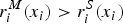 $r_i^M (x_i) \gt r_i^S (x_i)$ will be proved upon showing that a 1b 2 > a 2b 1, namely upon showing that
 $$\left [ {\lpar {1 + {\rho}} \rpar -\big( {{\beta}_i^M + {\rho} {\gamma\,}_i^M} \big) } \right ] \big( {{\beta}_i^S + {\rho} {\gamma\,}_i^S} \big) \gt \left [ {\lpar {1 + {\rho}} \rpar -\big( {{\beta}_i^S + {\rho} {\gamma\,}_i^S} \big) } \right ] \big( {{\beta}_i^M + {\rho} {\gamma\,}_i^M} \big) ,$$
which is equivalent to
 $$\lpar {1 + {\rho}} \rpar \big( {{\beta}_i^S + {\rho} {\gamma\,}_i^S} \big) \gt \lpar {1 + {\rho}} \rpar \big( {{\beta}_i^M + {\rho} {\gamma\,}_i^M} \big) ,$$
where the latter inequality holds by (8) in Lemma 2. Q.E.D.
Proof of Remark 1.
We re-apply Lemma 3 and employ the same substitutions as in the proof of Claim 1. The difference in the intensities of the relative risk aversion between an initially married individual and an initially single individual is given by
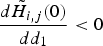
 $$r_i^M (x_i)-r_i^S (x_i) = H_i(0)-H_i(1).$$
 Upon closer inspection, in the preceding expression only 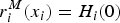 $r_i^M (x_i) = H_i(0)$ depends on the probability of divorce q. Hence, we can simplify:
 $$\displaystyle{{d \left [r_i^M (x_i)-r_i^S (x_i) \right ]} \over {dq}} = \displaystyle{{d \left [r_i^M (x_i) \right ] } \over {dq}} = \displaystyle{{dH_i(0)} \over {dq}}.$$
Furthermore, we have that
 $$\displaystyle{{dH_i(0)} \over {dq}} = \displaystyle{{dH_i(0)} \over {da_1}}\displaystyle{{da_1} \over {dq}} + \displaystyle{{dH_i(0)} \over {db_1}}\displaystyle{{db_1} \over {dq}}.$$
 Bearing in mind that 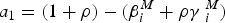 $a_1 = \lpar {1 + {\rho}} \rpar -\lpar {{\beta}_i^M + {\rho} {\gamma\,}_i^M} \rpar $ as well as using the definition of
  ${\gamma\,} _i^M $ in (4b), and drawing on the assumption
  ${\beta} _i^S \gt {\beta} _i^M $, we obtain that
 $$\displaystyle{{da_1} \over {dq}} = -{\rho} \big({\beta} _i^S -{\beta} _i^M \big) \lt 0.$$
 By analogy, we have that 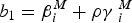 $b_1 = {\beta} _i^M + {\rho} {\gamma\,} _i^M $, hence
 $$\displaystyle{{db_1} \over {dq}} = {\rho} \big({\beta} _i^S -{\beta} _i^M \big) \gt 0.$$
 Because we have  $\displaystyle{{dH_i(0)} \over {da_1}} \gt 0$ by part II of Lemma 3, and
  $\displaystyle{{dH_i(0)} \over {db_1}} \lt 0$ by part III of Lemma 3, (22), (23), and (24) imply that
 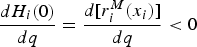 $\displaystyle{{dH_i(0)} \over {dq}} = \displaystyle{{d[r_i^M (x_i)]} \over {dq}} \lt 0$ and, hence, the difference in the levels of the relative risk aversion between an initially married individual and an initially single individual decreases in the probability of divorce. Q.E.D.
Proof of Claim 2.
To begin with, we show that condition (5) implies that
 $${\gamma\,} _i^M \lt {\gamma\,} _i^S. $$
 Indeed, the inequalities in (5) imply that  $q{\beta} _i^S \lt p{\beta} _i^M $ and that
  $(1-q + p){\beta} _i^M \lt (1-p + q){\beta} _i^S $. Then, from the definition of
  ${\gamma\,} _i^M $ in (4b), the following hold:
 $${\gamma\,} _i^M = (1-q){\beta} _i^M + q{\beta} _i^S \lt (1-q){\beta} _i^M + p{\beta} _i^M = (1-q + p){\beta} _i^M, $$
 $${\gamma\,} _i^M \lt (1-q + p){\beta} _i^M \lt (1-p + q){\beta} _i^S = (1-p){\beta} _i^S + q{\beta} _i^S \lt (1-p){\beta} _i^S + p{\beta} _i^M = {\gamma\,} _i^S. $$
Moreover, we note that
 $$\eqalign{& {\beta} _i^M {\gamma\,} _i^S = {\beta} _i^M \left [ {(1-p){\beta}_i^S + p{\beta}_i^M} \right ] \lt {\beta} _i^M \left [ {(1-p){\beta}_i^S + p{\beta}_i^S} \right ] = {\beta} _i^M {\beta} _i^S = \left [ {(1-q){\beta}_i^M + q{\beta}_i^M} \right ] {\beta} _i^S \cr & \;\;{\kern 1pt} \quad \;\;{\kern 1pt} \lt \left [ {(1-q){\beta}_i^M + q{\beta}_i^S} \right ] {\beta} _i^S = {\beta} _i^S {\gamma\,} _i^M} $$
or, in short, that
 $${\beta} _i^M {\gamma\,} _i^S \lt {\beta} _i^S {\gamma\,} _i^M. $$
Next, we look at the expected utility of an initially single individual as defined by (2a), namely
 $$\eqalign{& Ev_i^S \lpar {x_i,y_i} \rpar = (1-p)v_i^{S,S} \lpar {x_i,y_i} \rpar + pv_i^{S,M} \lpar {x_i,y_i} \rpar \cr & \ \quad \quad \quad \;{\kern 1pt} \; = (1-p)\big( {u_i^S (x_i) + {\rho} u_i^S (y_i)} \big) + p\big( {u_i^S (x_i) + {\rho} u_i^M (y_i)} \big) .} $$
 Because  $f(x_i) = ax_i^\lambda $, then it follows that
  $f\lpar {(1 + g_i)x_i} \rpar = a(1 + g_i)^\lambda x_i^\lambda = (1 + g_i)^\lambda \; f(x_i)$. Utilizing this equivalence, (28’) can be rewritten as
 $$\eqalign{& Ev_i^S \lpar {x_i,y_i} \rpar = {{\lcub}} \left[ {1 + {\rho} {(1 + g_i)}^\lambda} \right] -\Big[ {{\beta}_i^S + {\rho} {(1 + g_i)}^\lambda \,\big( {\,p{\beta}_i^M + (1-p){\beta}_i^S} \big) } \Big] {{\rcub}}\, f\,(x_i) \cr & \;\quad \;\quad \;\quad {\kern 1pt} -{\beta} _i^S RD_i\,({\bf x}) - \! {\rho} \left [ {\,p{\beta}_i^M + (1-p){\beta}_i^S} \right ] RD_i\,({\bf y})} $$
which, drawing on (4a), is equivalent to:
 $$Ev_i^S \lpar {x_i,y_i} \rpar = \left\{ \left[ {1 + {\rho} {(1 + g_i)}^\lambda} \right] -\left [ {{\beta}_i^S + {\rho} {(1 + g_i)}^\lambda {\gamma\,}_i^S} \right ]\right \} \, f\,(x_i)-{\beta} _i^S RD_i\,({\bf x})-{\rho} {\gamma\,} _i^S RD_i\,({\bf y}).$$
 Differentiating this last expression of  $Ev_i^S \lpar {x_i,y_i} \rpar $ with respect to x i yields
 $$\eqalign{& \displaystyle{{dEv_i^S (x_i,y_i)} \over {dx_i}} = \lcub {\lsqb {1 + \rho {(1 + g_i)}^\lambda} \rsqb -\lsqb {\beta_i^S + \rho {(1 + g_i)}^\lambda \gamma_i^S} \rsqb } \rcub {f}^{\prime}(x_i)-\lsqb {\beta_i^S + \rho (1 + g_i)\gamma_i^S} \rsqb \phi (i), \cr & \displaystyle{{d^2Ev_i^S (x_i,y_i)} \over {dx_i^2}} = \lcub {\lsqb {1 + \rho {(1 + g_i)}^\lambda} \rsqb -\lsqb {\beta_i^S + \rho {(1 + g_i)}^\lambda \gamma_i^S} \rsqb } \rcub {f}^{\prime \prime}(x_i).} $$
The formulae of the expected utility and of its first and second derivatives for an initially married individual, as well as the measures of the relative risk aversion of the individuals of the two types are modified accordingly.
Analogously to (19), we have that
 $$r_i^\mu (x_i) = \displaystyle{{-x_i{\,f}^{\prime \prime}(x_i)\left \{ {\left [ {1 + {\rho} {(1 + g_i)}^\lambda} \right ] -\left [ {{\beta}_i^\mu + {\rho} {(1 + g_i)}^\lambda \, {\gamma\,}_i^\mu} \right ] } \right \} } \over {\left \{ {\left [ {1 + {\rho} {(1 + g_i)}^\lambda} \right ] -\left [ {{\beta}_i^\mu + {\rho} {(1 + g_i)}^\lambda {\gamma\,}_i^\mu} \right ] } \right \} {\,f}^{\prime}(x_i)-\left [ {{\beta}_i^\mu + {\rho} (1 + g_i){\gamma\,}_i^\mu} \right ] { \phi} (i)}},$$
where μ ∈ {M,S}.
Once again we apply part I of Lemma 3 and substitute, this time as follows:
 $$\eqalign{& a_1 = \left [{1 + {\rho} {(1 + g_i)}^\lambda} \right ] -\left [ {{\beta}_i^M + {\rho} {(1 + g_i)}^\lambda {\gamma\,}_i^M} \right ] ,\quad \cr & a_2 = \left [{1 + {\rho} {(1 + g_i)}^\lambda} \right ] -\left [ {{\beta}_i^S + {\rho} {(1 + g_i)}^\lambda {\gamma\,}_i^S} \right ] ,} $$
 $$b_1 = {\beta} _i^M + {\rho} (1 + g_i){\gamma\,} _i^M, \quad b_2 = {\beta} _i^S + {\rho} (1 + g_i){\gamma\,} _i^S. $$
Applying a reasoning analogous to that in the proof of (7) in Lemma 2, it can be shown that a 1 and a 2 are positive. For instance, the inequality a 2 > 0 is implied by
 $$\eqalign{& {\beta} _i^S + {\rho} (1 + g_i)^\lambda {\gamma\,} _i^S = {\beta} _i^S + {\rho} (1 + g_i)^\lambda \left ( {\,p\,{\beta}_i^M + (1-p)\,{\beta}_i^S} \right ) \lt {\beta} _i^S + {\rho} (1 + g_i)^\lambda \left ( {\,p\,{\beta}_i^S + (1-p)\,{\beta}_i^S} \right ) \cr & \quad \quad \quad \quad \quad \quad \ \ \, {\kern 1pt} {\kern 1pt} {\kern 1pt} = {\beta} _i^S + {\rho} (1 + g_i)^\lambda {\beta} _i^S = {\beta} _i^S \left ( {1 + {\rho} {(1 + g_i)}^\lambda} \right ) \lt 1 + {\rho} (1 + g_i)^\lambda,} $$
and a 1 > 0 can be shown to hold similarly, bearing in mind that, obviously, b 1,b 2 > 0. Also the counterparts of the equalities in (21) hold. Consequently, the proof of the present claim will be completed upon showing that a 1b 2 > a 2b 1, namely that
 $$\eqalign{& \Big [ {\lpar {1 + {\rho} {\hat{g}}_i} \rpar -\left ( {{\beta}_i^M + {\rho} {\hat{g}}_i{\gamma\,}_i^M} \right ) } \Big ] \left [ {{\beta}_i^S + {\rho} (1 + g_i){\gamma\,}_i^S} \right ] \cr & \hskip-0.3pc\gt \Big [ {\lpar {1 + {\rho} {\hat{g}}_i} \rpar -\left ( {{\beta}_i^S + {\rho} {\hat{g}}_i{\gamma\,}_i^S} \right ) } \Big] \left [ {{\beta}_i^M + {\rho} (1 + g_i){\gamma\,}_i^M} \right ] ,} $$
where, to simplify, we substitute 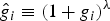 $\hat{g}_i\equiv (1 + g_i)^\lambda $. Upon rearranging, we get
 $$\eqalign{& \lpar {1 + \rho {\hat{g}}_i} \rpar \lpar {\beta_i^S -\beta_i^M} \rpar + \rho \lpar {1 + \rho {\hat{g}}_i} \rpar \lpar {1 + g_i} \rpar \lpar {\gamma_i^S -\gamma_i^M} \rpar \cr & \quad \quad \quad \quad \quad \quad \quad \;\;\; + \rho \lpar {1 + g_i-{\hat{g}}_i} \rpar \lpar {\beta_i^S \gamma_i^M -\beta_i^M \gamma_i^S} \rpar \gt 0.}$$
 The first term on the left hand-side of (30) is positive by the assumption that  ${\beta} _i^S \gt {\beta} _i^M $. The second term on the left hand-side of (30) is positive, because by (25) we have that
 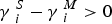 ${\gamma\,} _i^S -{\gamma\,} _i^M \gt 0$, and we know that 1 + g i > 0. As to the third term, we have, by assumption, that 0 < λ <1 and, hence,
  $1 + g_i \ge \hat{g}_i$, so that on recalling condition (28), we know that the third term is nonnegative. With inequality (30) shown to hold, the claim is proved. Q.E.D.
Proof of Remark 2.
We employ a reasoning that is analogous to the one given in (22) (see the proof of Remark 1). The only difference is that conditions (23) and (24) are replaced by
 $$\displaystyle{{da_1} \over {dq}} = -{\rho} \,(1 + g_i)^\lambda \left ({\beta} _i^S -{\beta} _i^M \right ) \lt 0$$
and
 $$\displaystyle{{db_1} \over {dq}} = {\rho} \,(1 + g_i) \left ({\beta} _i^S -{\beta} _i^M \right ) \gt 0.$$
 The inequalities in (31) and (32) hold because 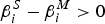 ${\beta} _i^S -{\beta} _i^M \gt 0$. By analogy to the proof of Remark 1, with (31) and (32) shown to hold, the proof is completed. Q.E.D.
Proof of Claim 3.
The proof is similar to the proof of Claim 2. First, we show that (6) implies that
 $$z {\gamma\,} _i^{M} \lt {\gamma\,}_i^{S}. $$
Indeed, analogously to (26), we have that
 $${\gamma\,} _i^{M} \lt (1 + q-p){\beta} _i^M. $$
 Because the first inequality in (6) implies that  $z(1-q + p){\beta} _i^M \lt (1-p + q){\beta} _i^S $, we have that
 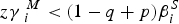 $z{\gamma\,} _i^{\,M} \lt (1-q + p){\beta} _i^S $ and, then, replicating the reasoning in (27) we get that
 $$z{\gamma\,} _i^{M }\le (1-q + p){\beta} _i^M \lt (1-p + q){\beta} _i^S = (1-p){\beta} _i^S + q{\beta} _i^S \le (1-p){\beta} _i^S + p{\beta} _i^M = {\gamma\,} _i^{S}. $$
We next show that
 $$z{\beta} _i^M \lt {\beta} _i^S .$$
 Indeed, because  ${{{\beta} _i^S} / {{\beta} _i^M}} \gt 1$, the second inequality in (6) implies that p > q. But this in turn implies that (1 + p − q)/(1 + q − p) >1 and, thus, by the first inequality in (6), we have that
 $$z \lt z\displaystyle{{1 + p-q} \over {1 + q-p}} \lt \displaystyle{{{\beta} _i^S} \over {{\beta} _i^M}}, $$
which proves that (35) holds.
Consider now the first and the second derivatives of the expected utility function of individual i. For ease of reference, we replicate the expected utility functions for a single individual and for a married individual, respectively:
 $$Ev_i^S \lpar {x_i,y_i} \rpar = (1-p)\left({u_i^S (x_i) + {\rho} u_i^S (y_i)} \right) + p\left( {u_i^S (x_i) + {\rho} u_i^M (y_i)} \right) ,$$
 $$Ev_i^M \lpar {x_i,y_i} \rpar = (1-q)\left( {u_i^M (x_i) + {\rho} u_i^M (y_i)} \right) + q\left( {u_i^M (x_i) + {\rho} u_i^S (y_i)} \right) .$$
Given the assumptions of the claim, we get that
 $$\eqalign{ Ev_i^S \lpar {x_i,y_i} \rpar &= {{\lcub}} {\Big[ {1 + {\rho} {(1 + g_i)}^\lambda} \Big] - \Big[ {{\beta}_i^S + {\rho} {(1 + g_i)}^\lambda \big( {\,p{\beta}_i^M + (1-p){\beta}_i^S} \big) } \Big] } {{\rcub}} \,f(x_i) \cr & \quad -{\beta} _i^S RD_i({\bf x}) - {\rho} \Big[ {\,p{\beta}_i^M + (1-p){\beta}_i^S} \Big] RD_i({\bf y}),} $$
 $$\eqalign{Ev_i^M \lpar {x_i,y_i} \rpar &= {{\lcub}} \Big[1 + {\rho} (1 + g_i)^\lambda \Big] -\Big[ {\beta}_i^M + {\rho} (1 + g_i)^\lambda \big( q{\beta}_i^S + (1-q){\beta}_i^M \big) \Big] {{\rcub}}\, f(x_i) \cr &\quad -{\beta} _i^M RD_i({\bf x})-{\rho} \Big [ {q{\beta}_i^S + (1-q){\beta}_i^M} \Big] RD_i({\bf y}).} $$
Differentiating these two expressions with respect to x i and substituting as per definitions (4a) and (4b) yields
 $$\eqalign{& \displaystyle{{dEv_i^\mu (x_i,y_i)} \over {dx_i}} = \lcub {\lsqb {1 + \rho {(1 + g_i)}^\lambda} \rsqb -\lsqb {\beta_i^\mu + \rho {(1 + g_i)}^\lambda \gamma_i^\mu} \rsqb } \rcub {f}^{\prime}(x_i)-\beta _i^\mu \phi (i)-\rho \gamma _i^\mu (1 + g_i)\phi (j), \cr & \displaystyle{{d^2Ev_i^\mu (x_i,y_i)} \over {dx_i^2}} = \lcub {\lsqb {1 + \rho {(1 + g_i)}^\lambda} \rsqb -\lsqb \beta_i^\mu + \rho {(1 + g_i)}^{\lambda \gamma_i^\mu} \rsqb } \rcub {f}^{\prime \prime}(x_i),} $$
where μ ∈ {M,S} and, therefore,
 $$r_i^\mu (x_i) = \displaystyle{{-x_i{\,f}^{\prime \prime}(x_i)\Big\{ {\Big[ {1 + {\rho} {(1 + g_i)}^\lambda} \Big] -\Big[ {{\beta}_i^\mu + {\rho} {(1 + g_i)}^\lambda {\gamma\,}_i^\mu} \Big] } \Big\} } \over {\Big\{ {\Big[ {1 + {\rho} {(1 + g_i)}^\lambda} \Big] -\Big[ {{\beta}_i^\mu + {\rho} {(1 + g_i)}^\lambda {\gamma\,}_i^\mu} \Big] } \Big\} {\,f}^{\prime}(x_i)-{\beta} _i^\mu {\phi} (i)-{\rho} {\gamma\,} _i^\mu (1 + g_i){\phi} (\,j)}}.$$
We can now apply part I of Lemma 4 and substitute as follows:
 $$\eqalign{& a_1 = \Big[ {1 + {\rho} {(1 + g_i)}^\lambda} \Big] -\Big[ {{\beta}_i^M + {\rho} {(1 + g_i)}^\lambda {\gamma\,}_i^M} \Big], \cr & a_2 = \Big[ {1 + {\rho} {(1 + g_i)}^\lambda} \Big] -\Big[ {{\beta}_i^S + {\rho} {(1 + g_i)}^\lambda {\gamma\,}_i^S} \Big] ,} $$
 $$c_1 = {\beta} _i^M, \quad c_2 = {\beta} _i^S, $$
 $$d_1 = {\rho} (1 + g_i){\gamma\,} _i^M, \quad d_2 = {\rho} (1 + g_i){\gamma\,} _i^S. $$
We note that the definitions of a 1 and a 2 are the same as in the proof of Claim 1 (in other words, (38a) and (29a) are identical) and, therefore, we have that a 1,a 2 > 0 by the same argument as the one employed in the proof of Claim 1. In addition, we obviously have that c 1,c 2 > 0, and that d 1,d 2 > 0. In order to complete the proof, we need to show that
 $$a_1(c_2 + d_2)\min \{ -{\phi} (i),-{\phi} (\,j)\} \gt a_2(c_1 + d_1)\max \{ -{\phi} (i),-{\phi} (\,j)\}, $$
which, upon substitution, translates into
 $$\eqalign{& \Big[ {\lpar {1 + {\rho} {\hat{g}}_i} \rpar -\big( {{\beta}_i^M + {\rho} {\hat{g}}_i{\gamma\,}_i^M} \big) } \Big] \Big[ {{\beta}_i^S + {\rho} (1 + g_i){\gamma\,}_i^S} \Big] \min \{ -{\phi} (i),-{\phi} (\,j)\} \cr & \hskip-0.2pc \gt \Big[ {\lpar {1 + {\rho} {\hat{g}}_i} \rpar -\big( {{\beta}_i^S + {\rho} {\hat{g}}_i{\gamma\,}_i^S} \big) } \Big] \Big[ {{\beta}_i^M + {\rho} (1 + g_i){\gamma\,}_i^M} \Big] \max \{ -{\phi} (i),-{\phi} (\,j)\},} $$
where, again, as we did just prior to (30), we substitute  $\hat{g}_i\equiv (1 + g_i)^\lambda $. Upon rearranging and substituting
 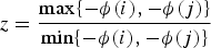 $z = \displaystyle{{\max \{ -{\phi} (i),-{\phi} (j)\}} \over {\min \{ -{\phi} (i),-{\phi} (j)\}}} $, we obtain the following equivalent expression:
 $$\eqalign{& \lpar {1 + {\rho} {\hat{g}}_i} \rpar \Big( {{\beta}_i^S -z{\beta}_i^M} \Big) + {\rho} \lpar {1 + {\rho} {\hat{g}}_i} \rpar \lpar {1 + g_i} \rpar \Big( {{\gamma\,}_i^S -z{\gamma\,}_i^M} \Big)+ {\rho} {\beta} _i^S {\gamma\,} _i^M \Big[ {z(1 + g_i)-{\hat{g}}_i} \Big] \cr & -{\rho} {\beta} _i^M {\gamma\,} _i^S \Big[ {(1 + g_i)-z{\hat{g}}_i} \Big] + (z-1){\beta} _i^S {\beta} _i^M + {\rho} ^2{\hat{g}}_i(1 + g_i){\gamma\,} _i^S {\gamma\,} _i^M (z-1) \gt 0.} $$
 On the left hand-side of (40) there are six terms. We already showed that the first two terms are positive (see (35) and (33), respectively), and because z ≥ 1 we know that the last two terms are nonnegative. So what remains to be evaluated are the signs of the middle two terms. To this end, we consider two cases. First, suppose that 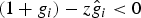 $(1 + g_i)-z\hat{g}_i \lt 0$. Then it follows that
  $-{\rho} {\beta} _i^M {\gamma\,} _i^S \lsqb {(1 + g)-z\hat{g}} \rsqb \gt 0$, and we infer that
 $${\rho} {\beta} _i^S {\gamma\,} _i^M \lsqb {z(1 + g_i)-{\hat{g}}_i} \rsqb -{\rho} {\beta} _i^M {\gamma\,} _i^S \lsqb {(1 + g_i)-z{\hat{g}}_i} \rsqb \gt 0$$
because both terms on the left hand-side of this last inequality are positive (we note that  $z(1 + g_i) \ge 1 + g_i \ge \hat{g}_i$). Second, suppose, alternatively, that
  $(1 + g_i)-z\hat{g}_i \ge 0$. It can then be easily checked that
  $z(1 + g_i)-\hat{g}_i \ge (1 + g_i)-z\hat{g}_i$, so we will have that
 $$\eqalign{& {\rho} {\beta} _i^S {\gamma\,} _i^M \Big[ {z(1 + g_i)-{\hat{g}}_i} \Big] -{\rho} {\beta} _i^M {\gamma\,} _i^S \Big[ {(1 + g_i)-z{\hat{g}}_i} \Big] \cr & \! \! \ge {\rho} \Big( {{\beta}_i^S {\gamma\,}_i^M -{\beta}_i^M {\gamma\,}_i^S} \Big) \Big[ {z(1 + g_i)-{\hat{g}}_i} \Big] \ge 0,} $$
where the second inequality in (40a) follows from (28) and, again, from  $z(1 + g_i) \ge \hat{g}_i$. We conclude that (40a) holds true and so does Claim 3. Q.E.D.
Proof of Remark 3.
We apply the same reasoning as in the proof of Remark 1, and we note that for Remark 3 to hold it suffices to show that  $\displaystyle{{d{\tilde{H}}_{ {i,j}}(0)} \over {dq}} \gt 0$, where the function
  $\tilde{H}_i(0)$ is defined by (13) and by the substitutions of (38a), (38b), and (38c).
It then follows that
 $$\displaystyle{{d{\tilde{H}}_{ {i,j}}(0)} \over {dq}} = \displaystyle{{d{\tilde{H}}_{ {i,j}}(0)} \over {da_1}}\displaystyle{{da_1} \over {dq}} + \displaystyle{{d{\tilde{H}}_{ {i,j}}(0)} \over {dc_1}}\displaystyle{{dc_1} \over {dq}} + \displaystyle{{d{\tilde{H}}_{ {i,j}}(0)} \over {dd_1}}\displaystyle{{dd_1} \over {dq}}.$$
 Because the substitution for a 1 is the same as in Remark 1, we have that  $\displaystyle{{da_1} \over {dq}} \gt 0$ by (31), and that
  $\displaystyle{{d{\tilde{H}}_{ {i,j}}(0)} \over {da_1}}\displaystyle{{da_1} \over {dq}} \lt 0$ by part II of Lemma 4. We also note that
  $\displaystyle{{dc_1} \over {dq}} = 0$. Finally, the definition of d 1 in (38c) implies (recalling (4b)) that
 $$\displaystyle{{dd_1} \over {dq}} = {\rho} (1 + g)\big({\beta} _i^S -{\beta} _i^M \big) \gt 0,$$
and, hence, we have that  $\displaystyle{{d{\tilde H}\,_{i,j}(0)} \over {dd_1}}\displaystyle{{dd_1} \over {dq}} \lt 0$ by part III of Lemma 4. In sum, we showed that the first and third terms on the right hand-side of (41) are negative, and that the middle term is equal to zero. Thus,
  $\displaystyle{{d{\tilde H}\,_{i,j}(0)} \over {dq}} \lt 0$ which, as we know from the proof of Remark 1, implies that the difference between the relative risk aversion of a married individual and the relative risk aversion of a single individual is declining in the probability of divorce. Q.E.D.

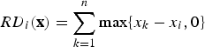


 Open access