


1. Introduction
Water impacts are responsible for extreme hydrodynamic forces on structures entering water. The critical loads relevant to the design of these structures in order to ensure their integrity arise at the highest water entry velocities. In these regimes, the flow is dominated by the fluid inertia. It is therefore common practice to neglect the other parameters of the water entry problem (e.g. surface tension, viscosity and gravity) when computing the loads arising in such harsh conditions with numerical models (e.g. Battistin & Iafrati Reference Battistin and Iafrati2003; Oger et al. Reference Oger, Doring, Alessandrini and Ferrant2006; Piro & Maki Reference Piro and Maki2011) or analytical models of water impact (Wagner Reference Wagner1932). In softer conditions, i.e. at lower entry velocity, but at a sufficiently small time scale such that the effect of viscosity and surface tension is still marginal, gravity may start affecting the results. Although not directly critical to the integrity of its structure, ‘soft’ slamming events may affect the motion of a falling (respectively floating) body subject to full (respectively partial) water entry. For example, floating marine structures may experience large amplitude motions and undergo slamming events induced by the relative motion between the body and the free surface, which in turn may affect the body motion. Kim et al. (Reference Kim, Kim, Yuck and Lee2015) and de Lauzon, Derbanne & Malenica (Reference de Lauzon, Derbanne and Malenica2019) have shown that the coupling of a water impact model (a generalized Wagner model) with the rigid-body motion of a container ship affected (limited) the pitch motion and, as a consequence, limited the whipping vibrations of the structure. The motion of wave energy converters (WEC) may also be affected by slamming loads. Babarit et al. (Reference Babarit, Mouslim, Clément and Laporte-Weywada2009) observed experimentally slamming events on the SEAREV WEC concept as soon as the pitch motion amplitude reached a value of  $10^{\circ }$ and reported that slamming forces limited the pitch motion of the device. Given the primary role played by gravity in the leading-order response of floating bodies to wave excitation loads, one may anticipate that gravity will also affect the slamming loads in these conditions. These kind of fluid–structure interactions may be seen as an intermediate regime between strongly nonlinear wave-structure interaction and pure slamming (when the effect of gravity is negligible).
Another field of application where gravity plays an important role during water impact events is the emergency landing on water of aircrafts. Indeed, despite very large horizontal velocity magnitudes, the hydrostatic term due to gravity in Bernoulli's equation is taken into account in the hydrodynamic models used to predict the motion of an aircraft during emergency landing on water, adding the term [ $-\rho g(z-z_0)$] when computing the pressure acting on the body (see Bensch et al. Reference Bensch, Shigunov, Beuck and Söding2001; Khabakhpasheva et al. Reference Khabakhpasheva, Korobkin, Maki and Seng2016; Martin, Jacques & Paul Reference Martin, Jacques and Paul2018), where $\rho$ is the liquid density and $z$ is the vertical coordinate of a point on the body surface. Formally speaking, for a two-dimensional body impacting a flat water surface located at $z=0$ (figure 1), the reference level $z_0$ should be set to 0. Note however that such a value leads to a suction effect (a negative contribution to the pressure) for $z>0$. Khabakhpasheva et al. (Reference Khabakhpasheva, Korobkin, Maki and Seng2016) obtained better force predictions for the water entry of a wedge with constant deceleration by setting $z_0=\eta (c(t),t)/2$, with $z=\eta (x,t)$ defining the free-surface elevation and $c(t)$ the half-width of the wetted surface within the Wagner model (see figure 1).

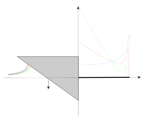
Figure 1. Water entry of a two-dimensional symmetric body.
In the generalized Wagner model (GWM) (see Helmers & Skeie Reference Helmers and Skeie2015; Kim et al. Reference Kim, Kim, Yuck and Lee2015; de Lauzon et al. Reference de Lauzon, Grgic, Derbanne and Malenica2015), which is commonly used to perform coupled slamming and hydroelastic sea-keeping computations, gravity is often neglected. In this context, adding the effect of gravity into the GWM is more challenging because gravity is already at play in the sea-keeping model and the coupling of the two models must be consistent.
Numerical approaches such as computational fluid dynamics (CFD) and fully nonlinear potential flow (FNPF) solvers may offer a more readily usable means of simulating water impacts affected by gravity as the introduction of gravity does not necessitate additional developments. In high-fidelity CFD approaches, the effect of gravity may be easily taken into account by adding a volumic force in the liquid domain. In FNPF solvers, taking into account gravity reduces to a modification of the free-surface boundary condition. Fully nonlinear potential flow solvers are less computationally demanding than CFD solvers while remaining at a high level of accuracy as the boundary conditions on the body and on the free surface are fully nonlinear. This approach has been used to investigate different water entry problems affected by gravity (Sun, Sun & Wu Reference Sun, Sun and Wu2015; Yu et al. Reference Yu, Xia, Jiao and Ren2018; Wang, Faltinsen & Lugni Reference Wang, Faltinsen and Lugni2019).
Despite the progress of high performance computing and CFD approaches, analytical and semi-analytical models (SAMs) of water impact remain highly valuable and under constant improvement. Indeed, they offer means of validation for numerical approaches through reference case studies within their domain of validity (i.e. small deadrise-angle wedge). Analytical and SAMs are used by industry not only because of their attractive computing performance but also because of their ability to deal with practical problems. Analytical models provide insights on complex flow physics such as the role of the longitudinal body curvature on the suction during oblique impacts and the possible appearance of cavitation (e.g. Bensch et al. Reference Bensch, Shigunov, Beuck and Söding2001; Tassin et al. Reference Tassin, Piro, Korobkin, Maki and Cooker2013; Martin et al. Reference Martin, Jacques and Paul2018). In that context, developing a consistent analytical model based on the Wagner approach but taking into account also the effect of gravity is of great interest. The difficulty resides in the fact that gravity not only changes the equation which gives the pressure acting on the body surface but it also changes the linearised free-surface boundary condition satisfied by the velocity potential ( $\varphi$) from $\varphi (|x|>c(t),z=0)=0$ to $\varphi _{,t}(|x|>c(t),z=0)=-g \eta (x,t)$. So one may ask whether it is legitimate to neglect the effect of gravity in the free-surface condition when the hydrostatic contribution to the pressure acting on the body becomes of importance. In order to answer this question, it is necessary to retain the gravity terms in the free-surface condition of the Wagner model and see how these terms affect the solution in terms of wetted surface width and pressure distribution. With the modified free-surface condition, the water entry problem becomes more difficult to solve because function $\eta (x,t)$, which describes the shape of the free surface, appears in the free-surface condition and becomes part of the unknowns of the problem. Moreover, with the modified free-surface condition, the velocity potential boundary condition at the free surface involves a time integral of function $\eta (x,t)$. As a consequence, the evaluation of the hydrodynamic load with the modified free-surface condition (with gravity) requires the knowledge of the time history of the wetted surface width, whereas the original Wagner model (without gravity) allows the evaluation of the wetted surface width and hydrodynamic load at any time independently from the previous time instants. It is only until very recently that a consistent Wagner model with gravity was proposed by Zekri, Korobkin & Cooker (Reference Zekri, Korobkin and Cooker2021) (see also Zekri Reference Zekri2016) for the water entry of a two-dimensional parabolic body using this modified free-surface condition and a perturbation method.
In the present article we present a more general approach for the derivation of a solution to the two-dimensional Wagner problem with gravity and we extend the theory to the axisymmetric water entry problem with gravity. This approach is used to investigate the water entry of wedges and cones of different deadrise angles but can be used to study the water entry of more general body shapes. The modified free-surface condition with gravity is taken into account when computing the contact point position,  $x=c(t)$, and when computing the velocity potential (and its partial derivatives) on the body surface. The so-called ‘Wagner problem’ which consists in determining the width of the wetted surface is rederived using the displacement potential approach with the new free-surface condition. The resolution of the Wagner problem is simplified by introducing an approximation of the free-surface condition which avoids the computation of the exact shape of the free surface with gravity. The two-dimensional Wagner problem is solved using analytical function theory and the axisymmetric Wagner problem is solved using the boundary element method (BEM) in a similar way as in Tassin et al. (Reference Tassin, Jacques, El Malki Alaoui, Nême and Leblé2012). The pressure acting on the body is computed according to the modified Logvinovich model (MLM) of Korobkin (Reference Korobkin2004). The semi-analytical approach is validated through comparisons with numerical results obtained from the FNPF solver presented in Battistin & Iafrati (Reference Battistin and Iafrati2004) and recently extended to deal with water impacts with varying speed and gravity (Del Buono et al. Reference Del Buono, Iafrati, Bernardini and Tassin2021). For this purpose, we investigate the effect of gravity during the water entry at constant speed of wedges and cones for different values of deadrise angle, $\beta$, ranging from $10^\circ$ to $30^\circ$. The comparisons between the two approaches are in very good agreement, hence demonstrating the accuracy of the semi-analytical approach. Our investigations show that accurately predicting the hydrodynamic force and the pressure distribution on the body requires us to account for gravity both in the modification of the wetted surface width and in the modification of the velocity potential. For the wedge entering water at constant speed, $V$, we show that the contribution of gravity to the non-dimensional force coefficient (the force multiplied by $\tan ^2\beta /(\rho V^3t)$) is governed by the effective Froude number, $F_r^*=Fr/\sqrt {\tan \beta }$, where $Fr=V/\sqrt {gh(t)}$ is the instantaneous Froude number based on the penetration depth, $h(t)$, taken as a reference length scale. The accuracy of the semi-analytical approach for the water entry of a body with a varying speed is also demonstrated through the simulation of a wedge and a cone entering water with deceleration (up to full stop). The motion imposed to the body in these simulations is similar to the one imposed in the experiments by Breton, Tassin & Jacques (Reference Breton, Tassin and Jacques2020) which were used in Del Buono et al. (Reference Del Buono, Iafrati, Bernardini and Tassin2021) to validate the FNPF solver. The simulations are run with and without gravity to show the capability of the SAM to accurately predict the effect of gravity on the force and the width of the wetted surface.
The article is organized as follows. Section 2 presents the two-dimensional semi-analytical water impact model. Section 3 describes the semi-analytical approach used for the axisymmetric water entry problem and § 4 presents the FNPF solver. The results obtained for the water entry at constant speed are presented in § 5 for the wedge case and in § 6 for the cone case. The results for a body entering water with deceleration are presented in § 7. Conclusions are finally drawn in § 8.
2. Two-dimensional analytical water impact model
In this section we present the two-dimensional analytical model developed to account for gravity. The original Wagner model without gravity is first recalled in § 2.1. The modified mixed boundary value problem (MBVP) satisfied by the velocity potential in the presence of gravity is presented and solved in § 2.2. In § 2.2.2 we derive the modified Wagner condition governing the evolution of the wetted surface and present the numerical approach used to solve this equation. The computation of the pressure and force acting on the body is detailed in § 2.2.3.
2.1. Two-dimensional Wagner model for a symmetric body
Within the Wagner model, the fluid is assumed to be inviscid and incompressible. Gravity and surface tension effects are neglected. The flow is assumed to be irrotational and can thus be fully described through a velocity potential  $\varphi$. Let us consider the water entry of a symmetric two-dimensional body into a semi-infinite liquid domain initially at rest as described in figure 1. The position of the body contour is defined by the equation $z=f(x)-h(t)$, where $f(x)$ is a function which describes the body shape and $h(t)$ corresponds to the depth of penetration after first contact with water. Variable $c(t)$ represents the half-width of the wetted surface, which is delimited by the turnover points or the root of the jets. Under Wagner's assumptions, the presence of the jet is neglected at leading order. The width of the wetted surface is determined using the so-called Wagner condition, which states that the displacement should be finite at $|x| = c$. Function $\eta (x,t)$ describes the elevation of the free surface induced by the water entry and the vertical velocity of the body is denoted $v(t)$. In the following, the upper-script notation $^{(w)}$ stands for quantities derived from the original Wagner model, i.e. neglecting gravity. In the original Wagner model, the velocity potential satisfies the following linear MBVP:
 $$\begin{gather} \Delta\varphi^{(w)} =0, \quad z<0, \end{gather}$$
 $$\begin{gather}\varphi^{(w)} = 0, \quad z=0, |x|\geqslant c^{(w)}(t), \end{gather}$$
 $$\begin{gather}\varphi_{,z}^{(w)} ={-}v(t), \quad z=0, |x|< c^{(w)}(t), \end{gather}$$
 $$\begin{gather}\varphi^{(w)} \rightarrow 0, \quad x^2+z^2\rightarrow\infty. \end{gather}$$
The velocity potential solution of (2.1) is given by the following expression on the body surface:
 \begin{equation} \varphi^{(w)}(x, z, t) ={-}v(t) \sqrt{c^{(w)}(t)^2-x^2},\quad \lvert x \rvert< c^{(w)}(t),\ z = 0. \end{equation}
Note however that the half-width of the wetted surface,  $c^{(w)}$, in (2.1) is a parameter which must be determined using an additional condition, the so-called Wagner condition, which can be formulated as (Korobkin Reference Korobkin1996)
 \begin{equation} \int_{0}^{{\rm \pi}/2} f(c^{(w)} \sin \gamma)\,\textrm{d} \gamma = \frac{\rm \pi}{2}h(t). \end{equation}
The free-surface elevation,  $\eta (x,t)$, can be obtained by integrating in time the vertical fluid velocity, $\varphi ^{(w)}_{,z}$, at the free surface, ( $|x|>c^{(w)}(t)$, $z=0$), (Faltinsen Reference Faltinsen2005)
 \begin{equation} \eta^{(w)}(x,t) =\int_0^t \varphi^{(w)}_{,z}(x,0,\tau)\,\textrm{d}\tau = \int_0^t \left[\frac{v(\tau)x}{\sqrt{x^2-c^{(w)}(\tau)^2}}-v(\tau) \right]\textrm{d}\tau. \end{equation}
For a number of body shapes (e.g. when  $f(x)$ is a polynomial function), a closed-form expression of $c^{(w)}$ can be derived using (2.3). As shown later in § 5, this expression can then be substituted into (2.4) to obtain a closed-form expression of the free-surface elevation.
2.2. Two-dimensional Wagner model with gravity
In the Wagner model the original nonlinear free-surface condition is first linearised assuming that there is a small deflection of the free surface and performing a Taylor expansion of the velocity potential in  $z=0$. This first step leads to the well-known free-surface condition of linear surface gravity waves,
 \begin{equation} \varphi_{,t}(x, z, t) ={-}g \eta(x,t), \quad |x|>c(t),z=0. \end{equation}
Neglecting gravity and assuming that the fluid is initially at rest, i.e.  $\varphi ^{(w)}(x,z,t=0$), one obtains the original free-surface condition $\varphi ^{(w)}=0$ in (2.1). Retaining the terms depending on gravity in the linear free-surface boundary condition, the MBVP satisfied by the velocity potential becomes
 $$\begin{gather} \Delta\varphi =0, \quad z<0, \end{gather}$$
 $$\begin{gather}\varphi(x,t) ={-}g \int_0^t\eta(x, \tau) \,\textrm{d}\tau, \quad z=0, |x|\geqslant c(t), \end{gather}$$
 $$\begin{gather}\varphi_{,z}(x,t) ={-}v(t),\quad z=0, |x|< c(t), \end{gather}$$
 $$\begin{gather}\varphi \rightarrow 0, \quad x^2+z^2\rightarrow\infty. \end{gather}$$
2.2.1. Derivation of the velocity potential accounting for gravity
Using the theory of analytic functions as detailed in Appendix A.1, the velocity potential solution of (2.6) on the wetted surface may be expressed as
 \begin{equation} \varphi(x, z, t) = \sqrt{c^2-x^2} \left\{{-}v+\frac{2}{\rm \pi}\int_{c}^{+\infty} \frac{\tau \varphi(\tau,t)}{\sqrt{\tau^2-c^2}(\tau^2-x^2)}\textrm{d}\tau \right\}, \quad |x|< c, z=0. \end{equation}
Note that the potential on the wetted surface depends on the potential on the free surface, which itself depends on the unknown free-surface elevation. The integrand in (2.7) is (weakly) singular at  $\tau = c$ for $x< c$. In order to compute the velocity potential, and more importantly the time derivative of the velocity potential close to $|x|=c^-$, it is convenient to rearrange (2.7) by performing an integration by parts, leading to
 \begin{align} \varphi(x, z, t) &={-}v\sqrt{c^2-x^2}+ \frac{2}{{\rm \pi} x} \left\{\textrm{sgn}(x)\frac{c \varphi(c^+, t) {\rm \pi}}{2}\right.\nonumber\\ &\quad \left.+\int_{c}^{+\infty} \arctan{\frac{\tau\sqrt{c^2-x^2}}{x\sqrt{\tau^2-c^2}}} (\varphi(\tau, t) +\tau \varphi_{,x}(\tau, t))\,{\rm d}\tau \right\}, \quad |x|< c, z=0. \end{align}
The time derivative of the velocity potential is obtained by differentiating (2.8) with respect to  $t$, leading to
 \begin{align} \varphi_{,t}(x, z,t) &= \frac{1}{\sqrt{c^2-x^2}}\left\{{-}v c\dot{c} + \int_{c}^{+\infty} \frac{2\tau \dot{c}}{{\rm \pi} c\sqrt{\tau^2-c^2}}(\varphi(\tau,t) +\tau \varphi_{,x}(\tau,t))\,{\rm d} \tau \right\}\nonumber\\ &\quad +\frac{c \varphi_{,t}(c^+,t) }{|x|} + \frac{2}{{\rm \pi} x}\int_{c}^{+\infty} \arctan{\frac{\tau\sqrt{c^2-x^2}}{x\sqrt{\tau^2-c^2}}} (\varphi_{,t}(\tau,t) +\tau \varphi_{,tx}(\tau,t))\,{\rm d} \tau\nonumber\\ &\quad -\dot{v}\sqrt{c^2-x^2}, \quad |x|< c, z=0, \end{align}
where the overdot symbol stands for the total derivative with respect to  $t$. The $x$-derivative of the velocity potential is obtained by solving the MBVP satisfied by the complex velocity ( $\varphi _{,x}-{\rm i}\varphi _{,z}$) using the theory of analytic functions as detailed in Appendix A.2. It yields
 \begin{equation} \varphi_{,x}(x, t) = \frac{x v}{\sqrt{c^2-x^2}}-\frac{2x}{{\rm \pi} \sqrt{c^2-x^2}} \int_{c}^{+\infty}\frac{\sqrt{\tau^2-c^2}}{\tau^2-x^2}\varphi_{,x}(\tau, t)\,\textrm{d}\tau, \quad |x|< c. \end{equation}
Equations (2.7) to (2.10) all involve the unknown free-surface elevation through the velocity potential on the free surface. Although gravity may affect the free-surface elevation, one may expect that the deviation of the free-surface elevation from the free-surface elevation obtained with the original Wagner model remains small as far as the effect of gravity remains reasonably small. As a consequence, it seems reasonable to assume that the leading-order terms of the velocity potential on the free surface can be computed using the free-surface elevation obtained with the original Wagner model. Note however that, as observed in Zekri et al. (Reference Zekri, Korobkin and Cooker2021), gravity will tend to reduce the size of the wetted surface; therefore, we suggest to assume that for a similar size of the wetted surface, the free surface obtained with gravity is approximately similar to the free-surface elevation obtained with the original Wagner model. In other words, at time  $t$, the half-width of the wetted surface with gravity, $c(t)$, is such that $c(t)=c^{(w)} (t^*)$, with $t^*< t$. The free-surface elevation which must be considered is thus $\eta (x,t) = \eta ^{(w)}(x,t^*)$. Denoting ${c^{(w)}}^{-1}$ the inverse function of ${c^{(w)}}$, we have $t^* = {c^{(w)}}^{-1}(c(t))$. The velocity potential on the free surface thus reads as
 \begin{equation} \varphi(x,t) ={-}g\int_0^t \eta(x,\tau) \,\textrm{d}\tau \approx{-}g\int_0^t \eta^{(w)}(x,{c^{(w)}}^{{-}1}[c(\tau)]) \,\textrm{d}\tau, \quad |x|>c, \end{equation}
The formal asymptotic analysis of Zekri et al. (Reference Zekri, Korobkin and Cooker2021) confirms that this approximation is reasonable. In Zekri et al. (Reference Zekri, Korobkin and Cooker2021) the free-surface shape is stretched to fit the new size of the wetted surface, but the idea is rather similar as the free-surface shape is assumed to be similar to the free-surface elevation given by the original Wagner model (in the stretched coordinates).
2.2.2. Modification of the wetted surface due to gravity
In order to take into account the effect of gravity on the wetted surface, it is convenient to reformulate the Wagner problem in terms of the displacement potential,  $\phi$, defined as the time integral of the velocity potential,
 \begin{equation} \phi(x, z, t) = \int_0^t \varphi(x, z, \tau) \,\textrm{d} \tau. \end{equation}
The displacement potential satisfies the following MBVP:
 $$\begin{gather} \Delta\phi =0, \quad z<0, \end{gather}$$
 $$\begin{gather}\phi =\int_0^t \varphi(x,\tau) \,\textrm{d} \tau, \quad z=0, |x|\geqslant c(t), \end{gather}$$
 $$\begin{gather}\phi_{,z} = f(x)-h(t),\quad z=0, |x|< c(t), \end{gather}$$
 $$\begin{gather}\phi \rightarrow 0, \quad x^2+z^2\rightarrow\infty. \end{gather}$$
This MBVP, in which the displacement potential is not equal to zero on the free surface, is solved in Moore, Ockendon & Oliver (Reference Moore, Ockendon and Oliver2013). A more detailed derivation of the solution is presented in Appendix B. Making a slightly different change of variable, the Wagner condition becomes
 \begin{equation} \int_{0}^{{\rm \pi}/2} \left( f(c \sin \gamma)-h(t) + \frac{\phi_{,x}\left(\dfrac{c}{\sin \gamma},t\right)}{\sin \gamma}\right)\textrm{d} \gamma = 0. \end{equation}
In the general case,  $c(t)$ cannot be extracted from the last term in (2.14) to express $c$ as a function of the other parameters because the term $\phi _{,x}$ on the free surface derives from successive integrals with respect to time. In order to solve this equation, it is convenient to differentiate (2.14) with respect to time, which leads to the following first-order differential equation:
 \begin{equation} \dot{c} ={-}\frac{\displaystyle\int_{0}^{{\rm \pi}/2} \left({-}v(t) +\phi_{,xt}\left.\left(\dfrac{c}{\sin \gamma},t\right)\right/\sin \gamma \right)\textrm{d} \gamma}{\displaystyle\int_{0}^{{\rm \pi}/2}\left( f_{,x}(c \sin \gamma)\sin \gamma + \phi_{,xx}\left.\left(\dfrac{c}{\sin \gamma},t\right)\right/\sin^2 \gamma\right)\textrm{d} \gamma}. \end{equation}
In the following this equation is solved numerically using the first-order explicit Euler method. Note that the wetted surface at a time instant  $t$ is fully determined by the position of the body $h(t)$ at this time instant through (2.3) when gravity is ignored. However, this is no longer true when gravity is considered because the displacement potential which appears in the second term of (2.14) is defined by a double integral over time. Similarly to § 2.2, we suggest using the free-surface elevation obtained from the original Wagner model in order to simplify the computation of the displacement potential in (2.15) as follows:
 \begin{align} \phi(x, t) & ={-}g\int_0^t \int_0^\nu \eta(x,\tau) \,\textrm{d}\tau \,\textrm{d}\nu \nonumber\\ &\approx{-}g\int_0^t \int_0^\nu \eta^{(w)}(x,{c^{(w)}}^{{-}1}(c(\tau)) \, \textrm{d}\tau \,\textrm{d}\nu, \quad |x|>c. \end{align}
Once the wetted surface and the partial derivatives of the velocity potential with respect to  $t$ and $x$ are known, it is possible to compute the pressure acting on the body.
2.2.3. Computation of the pressure and force acting on the body
In the following the pressure distribution is obtained using the MLM proposed by Korobkin (Reference Korobkin2004). This model allows us to take into account the shape of the body and was shown to be accurate in terms of hydrodynamic force prediction (Tassin et al. Reference Tassin, Jacques, El Malki Alaoui, Nême and Leblé2010). Writing the MLM under the form given in Tassin et al. (Reference Tassin, Piro, Korobkin, Maki and Cooker2013) and adding the hydrostatic component of Bernoulli's equation, the pressure acting on the body surface,  $P$, can be expressed as
 \begin{equation} P(x,t) ={-}\rho\left(\varphi_{,t} + \frac{\varphi_{,x}^2 } {2(1+f_{,x}^2)}+(f-h)\dot{v}+\frac{v^2}{2} + (f-h)g\right), \end{equation}
where  $\varphi _{,t}$ and $\varphi _{,x}$ are given by (2.9) and (2.10), respectively. This equation presents a non-integrable singularity at $|x| = c(t)^-$. In order to compute the force acting on the body, we follow the procedure proposed by Tassin et al. (Reference Tassin, Piro, Korobkin, Maki and Cooker2013) which consists in splitting (2.17) into two terms, $P_v$ and $P_a$, in the integration
 \begin{equation} F(t) = \int_{{-}c^*(t)}^{c^*(t)}P_v(x,t)\, \textrm{d} x + \int_{{-}c(t)}^{c(t)}P_a(x,t) \, \textrm{d} x, \end{equation}
where  $c^*(t)$ corresponds to the closest point $x$ to $c(t)$ where $P_v(x,t)$ is positive and $P_a$ comprises only terms depending on acceleration,
 \begin{equation} P_a ={-}\rho(\dot{v}\sqrt{c^2-x^2}+ (f-h) \dot{v}). \end{equation}
Here  $P_v$ comprises the remaining pressure terms and includes all the terms resulting from the action of gravity.
3. Axisymmetric analytical model
In this section the approach presented in the previous section in order to take into account the effect of gravity in the Wagner model is extended to the axisymmetric case. The axisymmetric model follows the same assumptions as the two-dimensional model, but the solution method differs because there is no equivalent theory to analytic function theory in three dimensions.
3.1. Axisymmetric Wagner model without gravity
The Wagner model also applies to the case of an axisymmetric body penetrating water where the problem is now expressed in the cylindrical coordinates  $(r,\theta,z)$. In the original axisymmetric Wagner problem, the velocity potential satisfies the following MBVP:
 $$\begin{gather} \Delta\varphi^{(w)} =0, \quad z<0, \end{gather}$$
 $$\begin{gather}\varphi^{(w)} = 0, \quad z=0, r\geqslant c^{(w)}(t), \end{gather}$$
 $$\begin{gather}\varphi^{(w)}_{,z} ={-}v(t), \quad z=0, r< c^{(w)}(t), \end{gather}$$
 $$\begin{gather}\varphi^{(w)} \rightarrow 0, \quad r^2+z^2\rightarrow\infty. \end{gather}$$
The velocity potential solution of (3.1) is given by the following expression on the body surface:
 \begin{equation} \varphi^{(w)}(r, \theta,z,t) = \frac{-2v}{\rm \pi} \sqrt{{c^{(w)}}^2-r^2}, \quad z = 0. \end{equation}
The radius of the wetted surface is governed by the Wagner condition which may be expressed as (see Korobkin & Scolan Reference Korobkin and Scolan2006)
 \begin{equation} \int_{0}^{{\rm \pi}/2}\sin \gamma {\cdot} f(c^{(w)}(t) \sin \gamma)\,\textrm{d} \gamma = h(t). \end{equation}
The vertical velocity at the free surface is given by Scolan & Korobkin (Reference Scolan and Korobkin2001) and reads as
 \begin{equation} \varphi_{,z}^{(w)}(r,\theta,z,t) = \frac{-2 v(t)}{\rm \pi}\left\{\arcsin\left(\frac{c^{(w)}(t)}{r}\right)-\frac{c^{(w)}(t)} {\sqrt{r^2-c^{(w)}(t)^2}}\right\}, \quad z = 0. \end{equation}
The free-surface elevation,  $\eta (r,t)$, can be obtained by integrating (3.4) with respect to time.
3.2. Axisymmetric Wagner model with gravity
Taking into account the effect of gravity in the axisymmetric Wagner problem, the velocity potential satisfies the following MBVP:
 $$\begin{gather} \Delta\varphi =0, \quad z<0, \end{gather}$$
 $$\begin{gather}\varphi ={-}g \int_0^t \eta(r,\tau)\,\textrm{d}\tau, \quad z=0, r\geqslant c(t), \end{gather}$$
 $$\begin{gather}\varphi_{,z} ={-}v(t), \quad z=0, r< c(t), \end{gather}$$
 $$\begin{gather}\varphi \rightarrow 0, \quad r^2+z^2\rightarrow\infty. \end{gather}$$
As the Laplace equation is linear, the velocity potential,  $\varphi$, solution of (3.5) may be sought in the form $\varphi =\varphi ^{(w)}+\varphi ^{(g)}$, with $\varphi ^{(g)}$ solution of the following MBVP:
 $$\begin{gather} \Delta\varphi^{(g)} =0,\quad z<0, \end{gather}$$
 $$\begin{gather}\varphi^{(g)} ={-}g \int_0^t \eta(r,\tau)\,\textrm{d}\tau, \quad z=0, r\geqslant c(t), \end{gather}$$
 $$\begin{gather}\varphi^{(g)}_{,z} = 0, \quad z=0, r< c(t), \end{gather}$$
 $$\begin{gather}\varphi^{(g)} \rightarrow 0, \quad r^2+z^2\rightarrow\infty. \end{gather}$$
 The normal derivative of the velocity potential being equal to zero over the disc  $r< c(t)$, the velocity potential on the wetted surface can be computed using the following equation given in Iafrati & Korobkin (Reference Iafrati and Korobkin2008) and referred to as Sneddon's formula:
 \begin{equation} \varphi^{(g)} (r, z ,t)= \frac{2}{\rm \pi} \int_0^{+\infty} \frac{\varphi^{(g)}(\sqrt{(c^2-r^2) \tau ^2 + c^2},z=0,t)}{\tau^2+1} \textrm{d} \tau, \quad r<c, z = 0. \end{equation}
Similarly to § 2, we suggest to approximate the free-surface elevation when computing the velocity potential over the free surface on the right-hand side of (3.7) as
 \begin{equation} \varphi^{(g)}(r, z,t) \approx{-}g\int_0^t \eta^{(w)}(r,{c^{(w)}}^{{-}1}(c(\tau)) \,\textrm{d}\tau, \quad r>c,z=0, \end{equation}
where  $\eta ^{(w)}(r,t)$ is obtained by integrating (3.4) with respect to time.
3.3. Modification of the wetted surface due to gravity
Similarly to the two-dimensional case, it is necessary to take gravity into account when computing the wetted surface radius (in the Wagner condition).
Moore & Oliver (Reference Moore and Oliver2014) proposed an analytical formulation to derive the wetted surface radius for an axisymmetric body considering a non-zero potential on the free surface. However, this paper contains an error and, for this reason, the formulation was not applied here. An erratum to the formulation should be published soon. Therefore, we suggest to adapt the numerical method based on the BEM proposed in Tassin et al. (Reference Tassin, Jacques, El Malki Alaoui, Nême and Leblé2012) in order to solve the modified Wagner problem with gravity.
3.3.1. Description of the method
The method presented here allows us to obtain the evolution of the wetted radius,  $c(t)$, during the vertical water entry of an axisymmetric body. The computation is made on a time interval, $[0, T]$, subdivided into $N$ subintervals. Time $t = 0$ corresponds to the instant at which the body first touches the water. Similarly to the two-dimensional case, obtaining the wetted radius at an instant $t_n$ necessitates to know the wetted radius at the previous instants $\{t_0,\dots, t_{n-1}\}$. Thus, an initialization must be made at the smallest instants of the impact for which no history has been computed. The Froude number, $Fr=\sqrt {V/(gt)}$, being much greater than one during the very early stage of the water entry, $c(t_n)$ is set to the value given by the Wagner theory at the first time instants (when the effect of gravity is marginal) in order to initialize the numerical procedure. Once the Froude number exceeds a certain threshold value, the wetted surface is determined numerically by an iterative procedure. This procedure consists in computing the free-surface elevation along the contact line for the successive values $c(t_n)_{m}$ corresponding to the value of $c(t_n)$ at each iteration $m$ and adjusting the value of the wetted surface radius so as to minimize the difference between the free-surface elevation and the body position along the contact line, i.e. the error on the Wagner condition.
This algorithm necessitates the computation of the free-surface elevation for a certain value of the wetted surface radius,  $c(t_n)_m$, which is performed by a boundary element model presented in § 3.3.2 below. In this computation the effect of gravity on the free-surface condition is taken into account and, thus, the computed free-surface elevation depends on the values taken by $c(t)$ at the previous instants $\{t_0,\dots, t_{n-1}\}$. Once the error on the Wagner condition has been computed, the estimate of $c(t_n)$ is updated following the procedure detailed in § 3.3.3. This procedure is then iterated until the error on the Wagner condition reaches a certain acceptable value.
3.3.2. Computation of the free-surface elevation
In order to calculate the free-surface elevation for a given value of the wetted surface radius,  $c(t)$, it is convenient to reformulate the Wagner problem in terms of the displacement potential, $\phi$, defined as the time integral of the velocity potential and which satisfies the following MBVP:
 $$\begin{gather} \Delta\phi =0, \quad z<0, \end{gather}$$
 $$\begin{gather}\phi =\int_0^t \varphi(r,\tau) \,\textrm{d} \tau,\quad z=0, r\geqslant c(t), \end{gather}$$
 $$\begin{gather}\phi_{,z} = f(r)-h(t), \quad z=0, r< c(t), \end{gather}$$
 $$\begin{gather}\phi \rightarrow 0, \quad r^2+z^2\rightarrow\infty. \end{gather}$$
Following Tassin et al. (Reference Tassin, Jacques, El Malki Alaoui, Nême and Leblé2012), the displacement potential at a point  $\boldsymbol {p}$ located at $z=0$ may be expressed as follows using Green's third identity:
 \begin{equation} \tfrac{1}{2}\phi(\boldsymbol{p},t) = \iint_{WS}\phi_{,z}(\boldsymbol{q},t)G(\boldsymbol{p},\boldsymbol{q}) \,\textrm{d}S_{\boldsymbol{q}} + \iint_{FS}\phi_{,z}(\boldsymbol{q},t)G(\boldsymbol{p},\boldsymbol{q}) \,\textrm{d}S_{\boldsymbol{q}}. \end{equation}
Here  $G(\boldsymbol {p},\boldsymbol {q})$ is the free-space Green function defined as $G(\boldsymbol {p},\boldsymbol {q}) =[4{\rm \pi} |\boldsymbol {p}-\boldsymbol {q}|]^{-1}$, $\boldsymbol {q}$ is a point located at $z=0$, $WS$ denotes the wetted surface and $FS$ denotes the free surface. Similarly to Tassin et al. (Reference Tassin, Jacques, El Malki Alaoui, Nême and Leblé2012), we use (3.10) and a collocation method to compute numerically the free-surface elevation, $\eta =\phi _{,z}$. The collocation method consists in enforcing (3.10) in a number of points $\boldsymbol {p}_i$ located on the free surface. The free surface is discretized in $N_e$ intervals over which the free-surface elevation is assumed to be piecewise linear,
 \begin{equation} \eta(\xi) = \frac{\eta(\xi_{k+1})-\eta(\xi_k)}{\xi_{k+1}-\xi_{k}} (\xi-\xi_k) +\eta(\xi_k), \quad \xi \in [\xi_k, \xi_{k+1}], \end{equation}
where  $\xi =r/c(t)$. The free-surface elevation is assumed to be small enough beyond a threshold value $\xi _{max}=5$ so that it has a marginal contribution to the second integral on the right-hand side of (3.10). Making use of this discretization, the integral on the free surface in (3.10) is split into $N_e+1$ terms corresponding to the coefficient of influence of each unknown, $\eta _k=\eta (\xi _k)$. The evaluation of (3.10) at $N_e+1$ collocation points $(\boldsymbol {p}_i)$ allows us to write the following linear system of equations:
 \begin{equation} \boldsymbol{A}\boldsymbol{X} = \boldsymbol{B}+ \boldsymbol{B}^{(g)}. \end{equation}
Here  $\boldsymbol {X}={(\eta _1,\ldots, \eta _{N_e+1})^{\rm T}}$, $\boldsymbol {A}$ results from the integral over the free surface in (3.10) and $\boldsymbol {B}$ results from the integration over the wetted surface. Their expression can be found in Tassin et al. (Reference Tassin, Jacques, El Malki Alaoui, Nême and Leblé2012). In contrast to Tassin et al. (Reference Tassin, Jacques, El Malki Alaoui, Nême and Leblé2012), an additional term $\boldsymbol {B}^{(g)}=1/2[\phi (\boldsymbol {p}_1),\ldots, \phi (\boldsymbol {p}_{N_e+1})]^{\rm T}$ appears because the displacement potential is not equal to 0 over the free surface when gravity is included. Similarly to (2.16), the displacement potential on the free surface may be approximated as
 \begin{align} \phi(\boldsymbol{p}_i,t) ={-}\int_0^t\int_0^\nu g \eta(\xi_{\boldsymbol{p}_i} c(\tau),\tau) \,\textrm{d}\tau \,\textrm{d}\nu \approx{-}\int_0^t\int_0^\nu g \eta^{(w)}(\xi_{\boldsymbol{p}_i} c(\tau),{c^{(w)}}^{{-}1}(c(\tau)))\,\textrm{d}\tau \,\textrm{d}\nu, \end{align}
where  $\eta ^{(w)}$ is obtained as the time integral of the vertical velocity (3.4). With this approximation, the $i$th coefficient of $\boldsymbol {B}^{(g)}$ at a time instant $t_{n+1}$ reads as
 \begin{equation} \boldsymbol{B}^{(g)}_i(t_{n+1}) ={-}\tfrac{1}{2}\int_0^{t_n}\int_0^\nu g \eta^{(w)}(\xi_{\boldsymbol{p}_i} c(\tau),{c^{(w)}}^{{-}1}(c(\tau)))\,\textrm{d}\tau \,\textrm{d}\nu, \end{equation}
where we only integrate with respect to time until  $t_n$ to avoid numerical issues at the first iteration (the free-surface elevation becomes singular when we set $c(t_{n+1})=c(t_n)$). The term $\boldsymbol {B}^{(g)}$ could be evaluated using the time history of the wetted surface elevation computed through the BEM. However, in order to obtain results valid under the same assumptions as in the two-dimensional case, it is evaluated using the analytical expression of the free-surface elevation, which also simplifies the computation. The resolution of the linear system (3.12) allows us to obtain the free-surface elevation at time $t_{n+1}$ assuming that $c(t_{n+1})=c(t_{n+1})_m$.
3.3.3. Enforcing the Wagner condition
Once the free-surface elevation has been computed, its value at the contact point is known and the corresponding error on the Wagner condition can be computed as
 \begin{equation} e(c(t_{n+1})_m) = \eta(\xi_0,t_{n+1})_m - f(c(t_{n+1})_m) + h(t_{n+1}). \end{equation}
For the next iteration, the value of  $c(t_{n+1})_m$ is updated as
 \begin{equation} c(t_{n+1})_{m+1} = c(t_{n+1})_m+ \alpha_m\,e(c(t_{n+1})_m), \end{equation}
where  $\alpha _m$ is a dynamic relaxation coefficient which is initialized and updated in a similar way as in Tassin et al. (Reference Tassin, Jacques, El Malki Alaoui, Nême and Leblé2012). The error resulting from the updated value $c(t_{n+1})_{m+1}$ can now be computed. This process is repeated until the error reaches an acceptable value. In our simulations, this procedure was initialized with $c(t_{n+1})_0=c(t_n)$, $c(t_n)$ being the converged value of $c(t)$ at $t=t_n$.
4. Fully nonlinear potential flow solver
In this section we present the FNPF model used to calculate the reference results for the validation of the two-dimensional and axisymmetric semi-analytical Wagner models with gravity. The FNPF model has been proposed and validated in Battistin & Iafrati (Reference Battistin and Iafrati2003) and Battistin & Iafrati (Reference Battistin and Iafrati2004) for the water entry case with constant velocity and extended in Del Buono et al. (Reference Del Buono, Iafrati, Bernardini and Tassin2021) to deal with the water impacts with varying speed and to include the effect of gravity. The solver is based on a hybrid BEM approach where the BEM is coupled with a harmonic polynomial expansion to describe the thinnest part of the jet.
4.1. Hybrid BEM approach
Similarly to the Wagner theory, the water impact problem is here faced under the assumptions of an inviscid and incompressible fluid. The flow is assumed irrotational, which allows us to formulate the problem in terms of the velocity potential  $\varphi$. The governing equations, written in an earth-fixed frame of reference, with $y$ the horizontal axis coinciding with the still water level, and $z$ the vertical axis oriented upwards, are
 $$\begin{gather} {\nabla^{2}\varphi} = 0, \quad \varOmega, \end{gather}$$
 $$\begin{gather}{\varphi,_{n}} ={-}\boldsymbol{v} \boldsymbol{\cdot} \boldsymbol{n}, \quad WS, \end{gather}$$
 $$\begin{gather}{\frac{{\rm D}\varphi}{{\rm D}t}} = {\frac{\left| \boldsymbol{\nabla} \varphi \right|^{2} }{2}-gz}, \quad FS, \end{gather}$$
 $$\begin{gather}{\frac{{\rm D}\boldsymbol{x}}{{\rm D}t}} = \boldsymbol{u}, \quad FS, \end{gather}$$
where  $\boldsymbol {v}$ is the body vertical velocity (positive downwards), $\varOmega$ is the fluid domain, $WS$ and $FS$ are the wetted surface and the free surface, respectively, $\boldsymbol {n}$ is the unit vector normal to the boundary of the fluid domain oriented inwards, ${{\rm D}}/{{\rm D}t}$ is the total derivative with respect to time $t$,
$t$,  $\boldsymbol {x}$ is the position of a particle lying at the free surface and $\boldsymbol {u}$ is the fluid velocity at $\boldsymbol {x}$. The problem is solved through a mixed Eulerian–Lagrangian approach inspired from Longuet-Higgins & Cokelet (Reference Longuet-Higgins and Cokelet1976) and the velocity potential is written in terms of a boundary integral representation. Enforcing it at the boundary of the fluid domain, a boundary integral equation of mixed first and second kind, for the velocity potential and its normal derivative on the free surface is obtained,
 \begin{equation}
\frac{1}{2}\varphi(\boldsymbol{p})=\int_{WS\bigcup
FS}{\left( \frac{\partial \varphi (\boldsymbol{p})}
{\partial \boldsymbol{n}} G(\boldsymbol{p},\boldsymbol{q})
-\varphi(\boldsymbol{q}) \frac{\partial
G(\boldsymbol{p},\boldsymbol{q})}{\partial \boldsymbol{n}}\right) {\rm
d}S_{\boldsymbol{q}}},
\end{equation}
\begin{equation}
\frac{1}{2}\varphi(\boldsymbol{p})=\int_{WS\bigcup
FS}{\left( \frac{\partial \varphi (\boldsymbol{p})}
{\partial \boldsymbol{n}} G(\boldsymbol{p},\boldsymbol{q})
-\varphi(\boldsymbol{q}) \frac{\partial
G(\boldsymbol{p},\boldsymbol{q})}{\partial \boldsymbol{n}}\right) {\rm
d}S_{\boldsymbol{q}}},
\end{equation}
where  $G$ is the free-space Green function for the Laplace operator. In two dimensions, the Green function is defined by $G(\boldsymbol {p},\boldsymbol {q}) = {\log (|\boldsymbol {p}-\boldsymbol {q}|)}/{2{\rm \pi} }$, and in three dimensions $G(\boldsymbol {p},\boldsymbol {q}) =[4{\rm \pi} |\boldsymbol {p}-\boldsymbol {q}|]^{-1}$. The solution is arranged in two steps. First, the boundary value problem formed by (4.1a), (4.1b) and the current value of the velocity potential at the free surface is solved. This provides the velocity potential on the wetted surface and its normal derivative on the free surface, along with the tangential velocity which is obtained through differentiation of the velocity potential along the boundary. Once the velocity field along the free surface is completely determined, the second step of the solution scheme is performed: the dynamic and kinematic free-surface conditions, (4.1c) and (4.1d), are integrated in time to compute the new free-surface shape and the velocity potential on it. The solution is achieved numerically through a zero-order discretization in space, thus approximating the variables with a piecewise constant distribution on straight panels, and a second-order Runge–Kutta scheme for the integration in time.
The hydrodynamic load acting on the impacting body is computed through the integration of the pressure distribution over the wetted surface, which is calculated by using the unsteady Bernoulli equation,
 \begin{equation} p-p_{inf}={-}\rho\left(\varphi_{,t}+\frac{\left| \boldsymbol{\nabla} \varphi \right|^{2} }{2}+gz \right), \end{equation}
where  $p_{inf}$ is the pressure on the undisturbed fluid. In (4.3) the time derivative of the velocity potential along the body, $\varphi _{,t}$, is unknown and it is evaluated by formulating a boundary value problem similar to (4.1) which is solved numerically by the BEM (see Battistin & Iafrati Reference Battistin and Iafrati2003).
4.2. Jet model
During the impact, the water rises along the body and a thin jet is formed due to the flow singularity at the intersection between the free surface and the body surface (Greenhow Reference Greenhow1987). An accurate modelling of this thin jet with the BEM approach would require a very fine local discretization and, owing to the local high speed of the fluid, a quite small time step would be necessary to guarantee the stability and the accuracy of the time integration scheme. Consequently, the computational effort would increase substantially. Commonly, for limiting the computational effort, the jet is cutoff and replaced by a panel orthogonal to the body contour where appropriate boundary conditions are applied. This procedure allows us to obtain, despite the approximation, an accurate estimation of the hydrodynamic load (Zhao & Faltinsen Reference Zhao and Faltinsen1993; Battistin & Iafrati Reference Battistin and Iafrati2003). However, an evident drawback is the loss of details in the description of the fluid motion inside the thin jet, which are important in some phenomena (e.g. flow separation). The jet model presented in Battistin & Iafrati (Reference Battistin and Iafrati2004) is adopted here to preserve a detailed description of the flow in the jet. This model is based on the discretization of a part of the jet region in control volumes, which are bounded by the wetted surface and the free surface (see figure 2), where the velocity potential is written in the form of a harmonic polynomial series, up to second order, about the corresponding centroid ( $x^*,z^*$),
 \begin{align} \varphi_{i}^j(x,z)&=A_i+B_i(x-x^*)+C_i(z-z^*)+\tfrac{1}{2}D_i[(x-x^*)^2 -(z-z^*)^2]\nonumber\\ &\quad +E_i(x-x^*)(z-z^*). \end{align}
Figure 2. Sketch of the jet region.
The coefficients  $A_{i},\ldots,E_{i}$ are additional unknowns, so five additional equations, for each control volume, are required. As the vertices of each volume correspond to the panel centroids ( $\bar {P}_{i-1}$, $\bar {P}_{i}$ on the body side, and $\hat {P}_{i-1}$, $\hat {P}_{i}$ on the free-surface side), four of them are derived by enforcing the boundary conditions at the body and free-surface sides,
 \begin{align} \varphi_{i,n}^j(\bar{P}_{i-1})=\varphi_{,n}(\bar{P}_{i-1}), \quad \varphi_{i,n}^j(\bar{P}_{i})=\varphi_{,n}(\bar{P}_{i}), \quad \varphi_{i}^j(\hat{P}_{i-1})=\varphi(\hat{P}_{i-1}), \quad \varphi_{i}^j(\hat{P}_{i})=\varphi(\hat{P}_{i}), \end{align}
where  $\varphi _{i,n}^j$ is the normal derivative of the velocity potential provided by the harmonic expression. The right-hand side of the first two equations of (4.5a–d) are known from the body boundary condition (4.1b), whereas the right-hand side of the last two equations of (4.5a–d) are known from the time integration of the dynamic boundary condition (4.1c), as explained in § 4.1. The fifth condition is the following matching condition which ensures the continuity of the normal derivative of the velocity potential (on the free-surface side) at adjacent control volumes,
 \begin{equation} \varphi_{i,n}^j(\hat{P}_{i-1})=\varphi_{(i-1),n}^j(\hat{P}_{i-1}). \end{equation}
It is worth noting that at the first edge on the free-surface side of the first control volume, the condition (4.6) enforces the matching of the normal derivative of the velocity potential computed by the simplified model with that resulting from the solution of the boundary integral problem.
By introducing the jet model, i.e. when the thin jet has already developed, the discretizated form of the boundary integral equation (4.2), used in the remaining part of the fluid domain, is coupled with the set of (4.5a–d) and (4.6). In this way, the unknown coefficients of the expansions and the unknown velocity potential and its normal derivative are computed simultaneously. This hybrid BEM approach is also adopted to compute numerically the time derivative of the velocity potential  $\varphi _{,t}$ which is needed to evaluate the pressure acting on the body contour.
5. Validation of the two-dimensional analytical model with gravity for a constant entry velocity
In this section we use the two-dimensional water impact model presented in § 2 to simulate the water entry of a wedge at constant speed and with the inclusion of gravity. In § 5.1 the equations presented in § 2 are further developed by making use of the closed-form solution provided by the original Wagner model in terms of wetted surface width and free-surface elevation. The results obtained for a  $15^\circ$ deadrise-angle wedge are presented and compared with the FNPF results in § 5.2. In § 5.3 a non-dimensional analysis of the problem is proposed to illustrate how the effect of gravity is governed by the effective Froude number defined as $Fr^* = Fr/\sqrt {\tan \beta }$.
5.1. Expression of the problem for the case of a wedge
The body shape of an infinite wedge is defined by the function
 \begin{equation} f(x) = \tan \beta |x|. \end{equation}
Substituting (5.1) into (2.3), the expression of the half-width of the wetted surface is obtained as
 \begin{equation} c^{(w)}(t) = \frac{{\rm \pi} h(t)}{2\tan \beta}. \end{equation}
Substituting (5.2) into (2.4) and integrating with respect to  $t$, we obtain the following expression for the free-surface elevation under the assumptions of the original Wagner model,
 \begin{equation} \eta^{(w)}(x,t) = \frac{2 \tan\beta}{\rm \pi}\left[x\arcsin{\frac{c^{(w)}(t)}{x}} -c^{(w)}(t)\right]. \end{equation}
Substituting (5.3) into (2.11), one obtains the following approximation for the velocity potential on the free surface:
 \begin{equation} \varphi(x, z , t) \approx{-}\frac{2 g \tan \beta}{\rm \pi} \int_{0}^{t} \left( x \arcsin{\frac{c(\tau)}{x}}- c(\tau) \right)\textrm{d} \tau, \quad |x| >c,z =0. \end{equation}
The expression of the velocity potential and its derivatives at the free surface can now be substituted into (2.9) and (2.10) in order to compute the pressure on the wetted surface and into (2.15) in order to compute the width of the wetted surface.
5.2. Water entry of a  $15^\circ$ deadrise-angle wedge at constant velocity and with gravity

In this section we investigate the water entry of a wedge with a deadrise angle of  $15^\circ$. The wedge enters water at a constant vertical velocity $v = 0.5\ {\rm m}\ {\rm s}^{-1}$. The evolution of the wetted surface half-width obtained from the SAM and the FNPF solver is depicted in figure 3(a). The results obtained from the two approaches neglecting gravity ( $g=0\ {\rm m}\ {\rm s}^{-2}$) are also depicted for comparison. One can see that gravity tends to reduce the size of the wetted surface and that the results obtained from the two approaches are in very good agreement. The latter is confirmed by the relative difference between the two approaches shown in figure 3(b). In the first instants, the relative difference is high because the FNPF simulation starts with a non-zero initial penetration depth which induces a short transitory stage at the beginning of the simulation. Then, the relative difference between the two approaches quickly decreases to $0.01\,\%$ for the case without gravity and to $0.5\,\%$ for the case with gravity. The pressure distributions obtained for different Froude numbers are depicted in figure 4(a). Note that the Froude number is defined as $Fr = V/\sqrt {g h(t)}$ and, therefore, the different instantaneous Froude numbers correspond to different time instants. Owing to the effect of gravity, the pressure is no longer self-similar. In fact, the peak pressure decreases in time (i.e. when the Froude number decreases) and its position changes. For small values of $Fr$, the maximum value of the pressure is no longer at the jet root but at the centre of the wedge where the hydrostatic contribution is maximum. The pressure distribution obtained by adding the term ‘ $-\rho g z$’ to the original MLM formulation, i.e. neglecting the effect of gravity on the wetted surface width and on the velocity potential, is also depicted in figure 4(a). This latter comparison shows how the new semi-analytical formulation improves the prediction of the pressure distribution compared with the more simplistic approach consisting in adding the hydrostatic contribution to the original MLM pressure model.

Figure 3. Comparison of the wetted surface half-width predicted by the SAM and the FNPF solver for a  $15^\circ$ deadrise-angle wedge entering water at constant velocity with and without gravity. (a) Evolution of the wetted surface half-width as a function of time. (b) Evolution of the relative difference between the two approaches, $(c_{FNPF} - c_{SAM})/c_{FNPF}$, as a function of time.

Figure 4. Comparison of the pressure coefficient,  $C_p = 2p/({\rho v^2})$, distribution along a $15^\circ$ deadrise-angle wedge entering water at constant speed. (a) Semi-analytical results accounting for the modification of the wetted surface due to gravity. (b) Semi-analytical results obtained using the wetted surface predicted by the original Wagner model. For comparison purposes, a dashed-dotted line computed as the sum of the hydrostatic term and the MLM has been added.
In order to illustrate the consequences of the wetted surface reduction under the action of gravity on the pressure distribution, the pressure distribution obtained at the same time instants with the SAM but neglecting the effect of gravity on the wetted surface are plotted in figure 4(b). This comparison clearly shows that taking into account gravity in the Wagner condition not only improves the prediction of the wetted surface width but also improves the overall prediction of the pressure distribution, and, in particular, the prediction of the pressure peak value. The force coefficient predictions obtained from the two approaches are depicted in figure 5(a). The relative difference between the two approaches is depicted in figure 5(b). A good agreement between the two models is obtained in terms of force, the relative difference remaining under  $4\,\%$. Most importantly, it is very interesting to note that the SAM remains very accurate in terms of force prediction even when the gravity contribution to the total force becomes of the same order of magnitude as the slamming force at infinite Froude number (figure 5a). The force prediction obtained by adding the hydrostatic force to the original MLM, which is also depicted in figure 5(a), is less accurate than the SAM with gravity. Note that adding the hydrostatic pressure term to the original MLM model leads to an underestimation of the pressure in the centre of the wedge and to an overestimation of the wetted surface (see figure 4), but by integrating the pressure over the wetted surface these two errors of opposite sign compensate partially each other and the force prediction appears to be reasonably good (see figure 5a).

Figure 5. Non-dimensional force acting on a wedge represented as a function of the inverse of the Froude number squared. (a) Force coefficient. (b) Relative difference  $(F_{SAM}-F_{FNPF})/F_{FNPF}$ between the semi-analytical results and the numerical results.
The results presented in this section showed that the SAM proposed in § 2 gives accurate results, both in terms of force and pressure distribution, for a wedge with a deadrise angle of  $15^\circ$ penetrating water vertically with a constant velocity. It appears that it is important to take into account the effect of gravity on the wetted surface to obtain an accurate prediction of both the pressure distribution and the resulting force. In the next section the effect of gravity during the water entry of wedges with different deadrise angles is investigated.
5.3. Relative influence of gravity during the water entry of a wedge at constant speed depending on the deadrise angle
In the previous section we observed that the action of gravity on the water entry of a  $15^\circ$ deadrise-angle wedge increased as the Froude number decreased. However, as shown by Yan & Liu (Reference Yan and Liu2011) in the case of a cone, one may expect that the importance of gravity at a given value of $Fr$ will differ for wedges of different deadrise angles. Indeed, based on the developments presented in Appendix C, we expect that the effect of gravity on the non-dimensional force coefficient and on the non-dimensional wetted surface width is governed by the non-dimensional parameter $Fr^* = Fr/\sqrt {\tan \beta }$, which we may refer to as the ‘effective Froude number’. Simulations of wedges entering water at constant velocity have been performed for deadrise-angle values ranging from 10 to $30^\circ$ with the SAM in order to confirm the primary role played by this parameter. The evolution of the force coefficient and of the gravity contribution to the non-dimensional force coefficient as a function of the inverse of the effective Froude number squared are depicted in figures 6(a) and 6(b), respectively. Comparisons with numerical results obtained from the FNPF solver for $\beta =10$, 15, 20 and $30^\circ$ are also shown. One can see that the semi-analytical results almost overlap and that the numerical results are in very good agreement with the semi-analytical ones, hence demonstrating that the importance of gravity during the water entry of a wedge is governed by the effective Froude number, $Fr^*$. The evolution of the non-dimensional half-width of the wetted surface is depicted in figure 7 as a function of the inverse of the effective Froude number squared. One can see that almost all the results overlap, hence confirming that the modification of the non-dimensional wetted surface half-width due to gravity is governed by the effective Froude number. Considering the effective Froude number thus allows us to account for the geometry of the impactor when estimating the relative effect of gravity.

Figure 6. Evolution of the non-dimensional force coefficient during the water entry of a wedge at constant velocity as a function of the inverse effective Froude number squared for different deadrise angles. (a) Total force coefficient and (b) gravitational component of the force coefficient. Here  $F_\infty$ denotes the force computed without including gravity, which is to say that the Froude number is infinite.

Figure 7. Evolution of the non-dimensional half-width of the wetted surface during the water entry of a wedge at constant velocity as a function of the inverse effective Froude number squared for different deadrise angles. (a) Non-dimensional half-width and (b) gravitational component of the half-width. Here  $c_\infty$ denotes the half-width of the wetted surface computed without including gravity, which is to say that the Froude number is infinite. The analytical results are so close that they are indistinguishable.
6. Validation of the axisymmetric model with gravity for a constant entry velocity
In this section we consider the water entry of a cone at constant velocity and with the inclusion of gravity. The axisymmetric model presented in § 3 is applied to this case. First, the wetted surface width is evaluated using the BEM presented in § 3. Then the potential on the wetted surface is computed analytically. In order to do so, it is necessary to compute the free-surface elevation obtained with the Wagner model which appears in (3.13). Within the original Wagner model, the wetted surface radius during the water entry of a cone is obtained by solving (3.3), which leads to
 \begin{equation} c^{(w)}(t) = \frac{4 h(t)}{{\rm \pi} \tan(\beta)}. \end{equation}
Substituting (6.1) into (3.4) and integrating with respect to time, we obtain the free-surface elevation corresponding to the original Wagner model (without gravity),
 \begin{equation} \eta^{(w)}(r, t) ={-}\frac{\tan \beta}{2} \left\{c^{(w)}(t)\arcsin\frac{c^{(w)}(t)}{r} +2\left(\sqrt{r^2-c^{(w)}(t)^2}-r\right)\right\}, \quad r>c. \end{equation}
Equation (6.2) is substituted into (3.13) to compute the radius of the wetted surface and into (3.8) to compute the velocity potential on the free surface. Within the computation of the wetted radius, the number of segments on the free surface was set to  $N_e = 30$ and $\xi _{max}$ was set equal to 10. The evolution of the radius of the wetted surface for a $15^\circ$ deadrise-angle cone is depicted in figure 8(a). The results without gravity are also depicted for the sake of comparison. Similarly to the two-dimensional case, the action of gravity tends to reduce the radius of the wetted surface. Figure 8(b) shows the relative difference between the semi-analytical results and the FNPF results. The models are in very good agreement as the relative difference for the case with gravity is under $0.4\,\%$. Once the evolution of the wetted surface accounting for gravity is known, the potential on the free surface is computed. This potential is then substituted into (3.7) to compute the velocity potential on the wetted surface and then to compute the pressure distribution. The pressure distributions obtained from the two approaches are depicted in figure 9(a). Figure 9(b) presents the pressure distribution obtained without accounting for the modification of the wetted surface in the SAM. The results obtained from the SAM are in good agreement with those obtained from the FNPF solver. Similarly to the two-dimensional case, it appears that not accounting for gravity in the wetted surface computation leads to an overestimation of the pressure peak magnitude and of the wetted surface radius. The non-dimensional force acting on the cone, which is obtained by integrating the pressure over the wetted surface, is depicted in figure 10(a). The gravity contribution to the non-dimensional force coefficient is depicted in figure 10(b), where the results obtained from the two approaches overlap. This indicates that the differences between the results observed in figure 10(a) are due to the intrinsic accuracy of the MLM in the axisymmetric case without gravity and not to the approach used to take gravity into account in the SAM. Similarly to the two-dimensional case, it is remarkable to see that the SAM remains very accurate in terms of force prediction even when the gravity contribution to the total force becomes of the same order of magnitude as the slamming force at infinite Froude number. The results obtained by adding the hydrostatic term to the MLM are closer to the SAM and FNPF results in the axisymmetric case than in the two-dimensional case, both in terms of pressure and force (see figures 9 and 10).

Figure 8. (a) Evolution of the wetted surface radius for a  $15^\circ$ deadrise-angle cone as a function of time obtained from the SAM and the FNPF solver with and without gravity. (b) Relative difference between the two approaches.

Figure 9. Comparison of the pressure coefficients,  $C_p = 2p/({\rho v^2})$, distribution along a $15^\circ$ deadrise-angle cone entering water at constant speed. (a) Semi-analytical results accounting for the modification of the wetted surface due to gravity. (b) Semi-analytical results obtained using the wetted surface predicted by the original Wagner model.

Figure 10. Comparison of the force coefficients for a  $15^\circ$ deadrise-angle cone entering water at constant speed. (a) Total force coefficient. (b) Gravity contribution to the force coefficient.
Semi-analytical and numerical simulations have been also carried out for different values of the cone deadrise angle. Figures 11(a) and 11(b) show the evolution of the non-dimensional wetted surface radius for different values of deadrise angle. The close agreement between the different curves shows that the wetted radius is mainly a function of the effective Froude number. The non-dimensional force results plotted in figure 12(a) and 12(b) confirm that the effect of gravity during the water entry of a cone is very well predicted by the effective Froude number and that the SAM with gravity performs well on a wide range of deadrise angles.

Figure 11. Evolution of the non-dimensional half-radius of the wetted surface during the water entry of a cone at constant velocity as a function of the inverse effective Froude number squared for different deadrise angles. (a) Total half-radius and (b) gravitational component of the half-radius.

Figure 12. Evolution of the non-dimensional force coefficient during the water entry of a cone at constant velocity as a function of the inverse effective Froude number squared for different deadrise angles. (a) Total force coefficient and (b) gravitational component of the force coefficient.
7. Results for a varying entry velocity
In this section we simulate the water entry of a  $15^\circ$ deadrise-angle wedge and a $15^\circ$ deadrise-angle cone with a varying entry velocity. The motion imposed to the body is similar to the motion of the water entry and exit experiments performed by Breton et al. (Reference Breton, Tassin and Jacques2020) with a $15^\circ$ deadrise-angle cone and is defined as
 \begin{equation} h(t) = H \sin(2{\rm \pi} t/T)-\delta_z, \end{equation}
where  $H = {{\rm \pi} c_{max} \tan \beta }/{4}$ is the maximum submergence depth, $T = {2{\rm \pi} H}/{U_{max}}$, $c_{max} = 0.2$ m is the maximum wetted surface half-width, $U_{max} = 0.57\ {\rm m}\ {\rm s}^{-1}$ is the maximum velocity and $\delta _z=3$ mm. Note that the body touches the water slightly after $t=0$ because of the term $\delta _z$ which has been introduced to reproduce the conditions of the experiments of Breton et al. (Reference Breton, Tassin and Jacques2020). A case with a smaller entry velocity has also been investigated in the following sections. For this case, the maximum velocity is taken as $U_{max} = 0.249 \ {\rm m}\ {\rm s}^{-1}$. In the following sections we investigate first the case of the wedge and then the case of the cone. Note that we focus on the entry stage in our investigations because the Wagner model is only valid as far as the wetted surface is in expansion. All the simulations have been carried out with and without gravity in order to highlight the effect of gravity in the simulations.
7.1. Decelerated water entry of a $15^\circ$ deadrise-angle wedge

The evolution of the wetted surface width during the water entry of the wedge, which is computed using (2.15), is depicted in figure 13 for the higher entry velocity  $U_{max} = 0.57 {\rm m}\ {\rm s}^{-1}$. The results obtained from the FNPF solver are also depicted. The results obtained from the two approaches without gravity are also plotted (blue lines) to show the effect of gravity. The initial discontinuity in the wetted surface radius prediction by the FNPF solver reflects the fact that the simulations start with a non-zero initial penetration depth. After this short transitory phase, the results obtained from the SAM and the FNPF solver without gravity are so close that it is hard to distinguish one from another. In this case, gravity has only a rather small effect on the radius of the wetted surface. Nevertheless, the reduction of the wetted surface radius under the action of gravity is well captured by the SAM. In figure 13 the time instant when the wetted surface stops expanding within the SAM is marked by a vertical dash-dotted line. In absence of gravity, the wetted surface stops expanding when the body stops moving downward within the Wagner model. However, both approaches (FNPF and SAM) predict that, under the action of gravity, the wetted surface stops expanding while the body continues moving downward. Gravity thus reduces the time during which the Wagner model can be applied. The pressure distributions along the wedge are depicted in figure 14(a) for a water entry with gravity and in figure 14(b) for a water entry without gravity. One can see that the semi-analytical results are in good agreement with the numerical results and that the SAM is able to predict the effect of gravity on the pressure distribution both when the pressure is positive (above atmospheric pressure) all over the body surface and when the pressure is negative (under atmospheric pressure). Note that the effect of gravity on the pressure distribution, which is rather small at the beginning of the water entry, increases with time. The force predictions resulting from these pressure distributions are depicted in figure 15(a). Consequently, the effect of gravity on the force, which is negligible in the first part of the entry, increases in time and affects the suction load. In order to demonstrate the ability of the SAM to accurately predict the effect of gravity on the force, the gravity contributions to the total force are depicted in figure 15(b), hence confirming that the differences observed between the semi-analytical and the numerical results in figure 15(a) are mainly due to the intrinsic accuracy of the MLM and not to a poor prediction of the effect of gravity. The results obtained using a lower entry velocity are depicted in figures 16 and 17 in terms of wetted surface radius and force. The maximum entry velocity is here taken as $U_{max} = 0.249\ {\rm m}\ {\rm s}^{-1}$. One can clearly see in figures 16 and 17 that the SAM is able to accurately predict the reduction of the wetted surface width under the action of gravity and the increase of the hydrodynamic force, respectively.

Figure 13. Evolution of the wetted surface radius during the decelerated water entry of a  $15^\circ$ deadrise-angle wedge ( $U_{max} = 0.57\ {\rm m} {\rm s}^{-1}$). The end of the wetted surface (WS) expansion corresponds to the instant at which the wetted surface width stops increasing. The Wagner model stops being valid at this instant.

Figure 14. Pressure distribution along a  $15^\circ$ deadrise-angle wedge at different time instants ( $U_{max} = 0.57\ {\rm m}\ {\rm s}^{-1}$). (a) Decelerated water entry with gravity. (b) Decelerated water entry without gravity.

Figure 15. Force evolution during the decelerated water entry of a  $15^\circ$ deadrise-angle wedge ( $U_{max} = 0.57\ {\rm m}\ {\rm s}^{-1}$). (a) Force evolution as a function of time. (b) Gravity contribution to the force.

Figure 16. Evolution of the wetted surface radius during the decelerated water entry of a  $15^\circ$ deadrise-angle wedge ( $U_{max} = 0.249\ {\rm m}\ {\rm s}^{-1}$). The end of the wetted surface (WS) expansion corresponds to the instant at which the wetted surface width stops increasing. The Wagner model stops being valid at this instant.

Figure 17. Force evolution during the decelerated water entry of a  $15^\circ$ deadrise-angle wedge ( $U_{max} = 0.249\ {\rm m}\ {\rm s}^{-1}$). (a) Force evolution as a function of time. (b) Gravity contribution to the force.
7.2. Decelerated water entry of a $15^\circ$ deadrise-angle cone

The results obtained for the water entry of the  $15^\circ$ deadrise-angle cone for $U_{max} = 0.57\ {\rm m}\ {\rm s}^{-1}$ in terms of wetted surface radius, pressure distribution and force are presented in figures 18, 19 and 20, respectively. The results obtained using a smaller entry velocity are depicted in figures 21 and 22 in terms of wetted surface radius and force for $U_{max} = 0.249\ {\rm m}\ {\rm s}^{-1}$. The number of segments on the free surface, $N_e$, defined in § 3.3.2, was taken equal to 40. We here took $\xi _{max} = 5$. Similarly to the two-dimensional case, the wetted surface radius predicted by the SAM is in good agreement with that predicted by the numerical model. The differences between the approaches observed in terms of pressure distribution are a bit more pronounced in the axisymmetric case than they were in the two-dimensional case. The force results show that the SAM underestimates the maximum (positive) force which appears at the beginning of the water entry. This difference, which is already visible in the constant velocity entry case (figure 10a), is amplified in the decelerated entry case. The gravity contribution to the force acting on the body predicted by the two approaches, as depicted in figures 20(b) and 22(b), are however in very good agreement.

Figure 18. Evolution of the wetted surface radius during the decelerated water entry of a  $15^\circ$ deadrise-angle cone ( $U_{max} = 0.57\ {\rm m} {\rm s}^{-1}$). The end of the wetted surface (WS) expansion corresponds to the instant at which the wetted surface radius stops increasing. The Wagner model stops being valid at this instant.

Figure 19. Pressure distribution along a  $15^\circ$ deadrise-angle cone at different time instants ( $U_{max} = 0.57\ {\rm m}\ {\rm s}^{-1}$). (a) Decelerated water entry with gravity. (b) Decelerated water entry without gravity.

Figure 20. Force evolution during the decelerated water entry of a  $15^\circ$ deadrise-angle cone ( $U_{max} = 0.57\ {\rm m}\ {\rm s}^{-1}$). (a) Force evolution as a function of time. (b) Gravity contribution to the force.

Figure 21. Evolution of the wetted surface radius during the decelerated water entry of a  $15^\circ$ deadrise-angle cone ( $U_{max} = 0.249\ {\rm m} {\rm s}^{-1}$). The end of the wetted surface (WS) expansion corresponds to the instant at which the wetted surface width stops increasing. The Wagner model stops being valid at this instant.

Figure 22. Force evolution during the decelerated water entry of a  $15^\circ$ deadrise-angle cone ( $U_{max} = 0.249\ {\rm m}\ {\rm s}^{-1}$). (a) Force evolution as a function of time. (b) Gravity contribution to the force.
8. Conclusions
We have presented an extension to the Wagner model in order to take into account the effect of gravity during the water entry of two-dimensional and axisymmetric bodies. For this purpose, the free-surface condition of the Wagner model has been modified by retaining the terms due to gravity. In the model this modified condition affects both the computation of the velocity potential (and its derivatives) and the size of the wetted surface. In two-dimensions the problem is solved using the theory of analytic functions. In particular, the Wagner problem is reformulated using the displacement potential. For the axisymmetric case, we use the Sneddon formula derived by Iafrati & Korobkin (Reference Iafrati and Korobkin2008) in order to solve the MBVP with non-zero potential at the free surface satisfied by the velocity potential. The radius of the wetted surface is computed by a boundary element model adapted from the approach presented in Tassin et al. (Reference Tassin, Jacques, El Malki Alaoui, Nême and Leblé2012). In order to simplify the computation of the free-surface condition, i.e. the potential at the free surface, we have proposed an approximation of the free-surface elevation with gravity based on the free-surface elevation derived from the original Wagner model (without gravity), which can be computed beforehand for a certain value of the wetted surface width (or radius). The semi-analytical approach has been implemented for a wedge and a cone, which makes it possible to develop further the expressions of the free-surface condition. The approach can however be generalized to arbitrary body shapes (including discretized body shapes), for example, by computing tabulated values of the free-surface elevation by the Wagner model for given values of the wetted surface width or radius.
Two-dimensional and axisymmetric FNPF simulations have been carried out to validate the SAM of water impact with gravity. All the simulations have been carried out with and without gravity in order to highlight the effect of gravity in the simulations. These comparisons demonstrate that the SAM performs well in terms of pressure distribution and force predictions on a wide range of wedge and cone water entry cases at constant velocity ( $\beta =10^\circ$ to $30^\circ$). Our simulations show that it is both important to take gravity into account when computing the velocity potential and the wetted surface width/radius in order to compute accurately the pressure distribution and the force. The gravity contribution to the force coefficient for wedges of different deadrise angles has been shown to be governed by the effective Froude number defined as $Fr^*=Fr/\sqrt {\tan \beta }$. The results obtained for a $15^\circ$ deadrise-angle cone entering water at constant velocity are also very satisfactory.
The SAM has been also used to investigate the decelerated water entry of a  $15^\circ$ deadrise-angle wedge and a $15^\circ$ deadrise-angle cone with gravity, until full stop. The results show that the SAM is able to predict accurately the effect of gravity during a decelerated water entry. In particular, similarly to the numerical model, the SAM predicts that, under the action of gravity, the wetted surface stops expanding while the body is still moving downward. The results obtained from the SAM are less accurate for the cone than for the wedge. In particular, our results show that the maximum (positive) force at the beginning of the decelerated cone water entry is underestimated by the SAM, both with and without gravity. The gravity contribution to the force coefficient is however well captured by the SAM, both in the two-dimensional and axisymmetric cases.
Funding
This work was supported by ISblue project, Interdisciplinary graduate school for the blue planet (ANR-17-EURE-0015) and co-funded by a grant from the French government under the program ‘Investissements d'Avenir’.
Declaration of interests
The authors report no conflict of interest.
Appendix A. Derivation of the velocity potential and of its $x$-derivative

A.1. Derivation of the velocity potential accounting for gravity (2.7)
In order to solve (2.6), let us introduce the complex potential  $\varPhi _1$ defined as
 \begin{equation} \varPhi_1(\xi) = \varphi(x,z)+{\rm i}\psi(x,z), \end{equation}
where  $\varphi$ is the velocity potential solution of (2.6) and $\psi$ is the streamfunction defined such that $\varphi$ and $\psi$ satisfy the Cauchy–Riemann equations. Potential $\varPhi _1$ is therefore analytic and the results on analytic functions can be applied to $\varPhi _1$. Let us now introduce the new unknown analytic function $H_1$ defined as
 \begin{equation} H_1(\xi) = \frac{\varPhi_1(\xi)}{\sqrt{\xi^2-c^2}}, \end{equation}
where  $\xi = x+{\rm i}z$. The values of the characteristic function $\sqrt {\xi ^2-c^2}$ on the real axis ( $z=0$) are given by
 $$\begin{gather} \sqrt{\xi^2-c^2}={-}\sqrt{x^2-c^2},\quad x<{-}c,z=0, \end{gather}$$
 $$\begin{gather}\sqrt{\xi^2-c^2}=\sqrt{x^2-c^2},\quad x>c,z=0, \end{gather}$$
 $$\begin{gather}\sqrt{\xi^2-c^2}={-}{\rm i}\sqrt{c^2-x^2}, \quad |x|< c,z=0^-, \end{gather}$$
 $$\begin{gather}\sqrt{\xi^2-c^2}={\rm i}\sqrt{c^2-x^2},\quad |x|< c,z=0^+. \end{gather}$$
The real part of  $H_1$ on the real axis is given by
 $$\begin{gather} {\rm Re}[H_1(x+{\rm i}0^-)] = \frac{-\varphi(x,0)}{\sqrt{x^2-c^2}}, \quad x<{-}c, \end{gather}$$
 $$\begin{gather}{\rm Re}[H_1(x+{\rm i}0^-)] = \frac{-\psi(x,0)}{\sqrt{c^2-x^2}},\quad |x|< c, \end{gather}$$
 $$\begin{gather}{\rm Re}[H_1(x+{\rm i}0^-)] = \frac{\varphi(x,0)}{\sqrt{x^2-c^2}}, \quad x>c. \end{gather}$$
Moreover,  $H_1=O(|\xi |^{-2})$ as $|\xi | \rightarrow {} \infty$. Thus, $H_1$ satisfies a MBVP whose solution is given by Hilbert's formula as
 \begin{equation} H_1(\xi) = \frac{{\rm i}}{\rm \pi} \int_{-\infty}^{+\infty} \frac{{\rm Re}[H_1(\tau+{\rm i}0^-)]}{\tau-\xi}\textrm{d}\tau. \end{equation}
By applying the Sokhotsky–Plemelj's formula, one obtains the limit of  $H_1$ at $z = 0^-$ as
 \begin{equation} H_1(x+{\rm i}0^-) = {\rm Re}[H_1(x+{\rm i}0^-)] + \frac{{\rm i}}{\rm \pi} {\int\hskip -1,05em -\,}_{-\infty}^{+\infty}\frac{{\rm Re}[H_1(\tau+{\rm i}0^-)]}{\tau-x} \textrm{d}\tau, \end{equation}
where the dashed integral sign denotes the Cauchy principal value. Using (A3) and (A2),  $H_1$ can also be written as
 \begin{equation} H_1(x,0^-) = \frac{{\rm i}\varphi(x,0^-)}{\sqrt{c^2-x^2}}-\frac{\psi(x,0^-)} {\sqrt{c^2-x^2}}, \quad |x|< c. \end{equation}
By identifying the real and imaginary parts, one obtains
 \begin{align} \varphi(x,0^-) &= \frac{\sqrt{c^2-x^2}}{\rm \pi} {\int\hskip -1,05em -\,}_{-\infty}^{+\infty}\frac{{\rm Re}[H_1(\tau+{\rm i}0^-)]}{\tau-x} \textrm{d}\tau\nonumber\\ &= \frac{\sqrt{c^2-x^2}}{\rm \pi} \left\{ \underbrace{\displaystyle\int_{-\infty}^{{-}c} \frac{-\varphi(\tau)}{\sqrt{\tau^2-c^2}(\tau-x)} \textrm{d}\tau}_{I_1(x)} \underbrace{+\displaystyle{\int\hskip -1,05em -\,}_{{-}c}^{c} \frac{-\psi(\tau)}{ \sqrt{c^2-\tau^2}(\tau-x)} \textrm{d} \tau}_{I_2(x)} \right. \nonumber\\ &\quad\left.+ \underbrace{\displaystyle\int_{c}^{+\infty}\frac{\varphi(\tau)}{\sqrt{\tau^2-c^2}(\tau-x)} \textrm{d}\tau}_{I_3(x)} \right\}, \end{align}
where  $I_2(x)=-{\rm \pi} v/2$. Rearranging $I_1$ and $I_3$, one obtains the velocity potential in the form of (2.7).
A.2. Derivation of the $x$-derivative of the velocity potential accounting for gravity

Let us introduce the complex velocity potential  $\phi _2$ defined as
 \begin{equation} \phi _2 = \varphi_{,x}(x,z)-{\rm i}\varphi_{,z}(x,z) \end{equation}
and function  $H_2$ defined as
 \begin{equation} H_2(\xi) = \phi _2(\xi) \sqrt{\xi^2-c^2}. \end{equation}
The real part of  $H_2$ on the real axis is
 $$\begin{gather} {\rm Re}[H_2(x+{\rm i}0^-)] = \varphi_{,x} \sqrt{x^2-c^2}, \quad x>c, \end{gather}$$
 $$\begin{gather}{\rm Re}[H_2(x+{\rm i}0^-)] ={-}\varphi_{,x} \sqrt{x^2-c^2}, \quad x<{-}c, \end{gather}$$
 $$\begin{gather}{\rm Re}[H_2(x+{\rm i}0^-)] ={-}\varphi_{,z} \sqrt{c^2-x^2}, \quad |x|<c. \end{gather}$$
Using Hilbert's formula and Sokhotsky–Plemelj's formula as in the previous section, we obtain  $\varphi _{,x}$ on the wetted surface,
 \begin{align} \varphi_{,x}(x, z) &=\frac{-1}{{\rm \pi} \sqrt{c^2-x^2}} \int_{-\infty}^{+\infty} \frac{{\rm Re}[H_2(\tau+{\rm i}0^-)]}{\tau-x} \textrm{d}\tau\nonumber\\ &= \frac{-1}{{\rm \pi} \sqrt{c^2-x^2}} \left\{ \underbrace{\int_{-\infty}^{{-}c}\frac{-\sqrt{\tau^2-c^2}\varphi_{,x}(\tau)}{\tau-x} \textrm{d}\tau}_{I_{1}(x)} \underbrace{+{\int\hskip -1,05em -\,}_{{-}c}^{c} \frac{-\sqrt{c^2-\tau^2}\varphi_{,z}(\tau)}{\tau-x} \textrm{d} \tau}_{I_{2}(x)} \right. \nonumber\\ &\quad \left.+ \underbrace{\int_{c}^{+\infty}\frac{\sqrt{\tau^2-c^2}\varphi_{,x}(\tau)}{\tau-x} \textrm{d}\tau}_{I_{3}(x)} \right\}, \quad x< c, z = 0, \end{align}
with  $I_{2}(x) = -{\rm \pi} x v$ for a rigid body. Rearranging $I_{1}(x)+I_{3}(x)$ leads to
 \begin{equation} \varphi_{,x}(x, z) = \frac{x V}{\sqrt{c^2-x^2}}-\frac{2x}{{\rm \pi} \sqrt{c^2-x^2}} \int_{c}^{+\infty}\frac{\sqrt{\tau^2-c^2}}{\tau^2-x^2}\varphi_{,x}(\tau)\,\textrm{d}\tau, \quad |x|< c, z = 0. \end{equation}
Appendix B. Modified Wagner condition with gravity in two dimensions
In order to derive the modified Wagner condition, let us introduce the new unknown analytic function  $H_4$ defined as
 \begin{equation} H_4(\xi) = \sqrt{\xi^2-c^2}[\phi_{,x}(\xi) - {\rm i}\phi_{,z}(\xi)], \end{equation}
where  $\phi$ is the displacement potential solution of (2.13). Using (A3), one obtains the real part of $H_4$ on the real axis,
 $$\begin{gather} {\rm Re}[H_4(x+{\rm i}0^-)] ={-}\phi_{,x} \sqrt{x^2-c^2}, \quad x<{-}c, \end{gather}$$
 $$\begin{gather}{\rm Re}[H_4(x+{\rm i}0^-)] ={-}\phi_{,z} \sqrt{c^2-x^2}, \quad |x|< c, \end{gather}$$
 $$\begin{gather}{\rm Re}[H_4(x+{\rm i}0^-)] = \phi_{,x} \sqrt{x^2-c^2}, \quad x>c. \end{gather}$$
Given that  $\phi _{,x}(\xi ) = O(|x^2+z^2|^{-1})$, we have $H_4(\xi ) \underset {\xi \rightarrow \infty }{\rightarrow } 0$. The imaginary part of $H_4$ on the $x$-axis is given by
 $$\begin{gather} {\rm Im}[H_4(x+{\rm i}0^-)] = \sqrt{x^2-c^2}\phi_{,z}(x,0), \quad x<{-}c, \end{gather}$$
 $$\begin{gather}{\rm Im}[H_4(x+{\rm i}0^-)] ={-}\sqrt{x^2-c^2}\phi_{,z}(x,0), \quad x>c. \end{gather}$$
The solution of this MBVP on the  $x$-axis is
 \begin{equation} H_4(x+{\rm i}0^-) = {\rm Re}[H_4(x+{\rm i}0^-)] + \frac{{\rm i}}{\rm \pi} \int_{-\infty}^{+\infty} \frac{{\rm Re}[H_4(\tau+{\rm i}0^-)]}{\tau-x} \textrm{d} \tau. \end{equation}
By identifying the imaginary part of the potential on both sides of (B4), the vertical displacement can be expressed as
 \begin{equation} \phi_{,z} =
\begin{cases} \dfrac{1}{\sqrt{x^2-c^2}} \dfrac{1}{\rm \pi}
\displaystyle\int_{-\infty}^{+\infty}\frac{{\rm
Re}[H_4(\tau+{\rm i}0^-)]}{\tau-x} \textrm{d} \tau, &
\text{ $x<{-}c$,}\\
-\dfrac{1}{\sqrt{x^2-c^2}}\dfrac{1}{\rm \pi}
\displaystyle\int_{-\infty}^{+\infty}\frac{{\rm Re}
[H_4(\tau+{\rm i}0^-)]}{\tau-x} \textrm{d} \tau, & \text{
$x>c$}.\\ \end{cases} \end{equation}
\begin{equation} \phi_{,z} =
\begin{cases} \dfrac{1}{\sqrt{x^2-c^2}} \dfrac{1}{\rm \pi}
\displaystyle\int_{-\infty}^{+\infty}\frac{{\rm
Re}[H_4(\tau+{\rm i}0^-)]}{\tau-x} \textrm{d} \tau, &
\text{ $x<{-}c$,}\\
-\dfrac{1}{\sqrt{x^2-c^2}}\dfrac{1}{\rm \pi}
\displaystyle\int_{-\infty}^{+\infty}\frac{{\rm Re}
[H_4(\tau+{\rm i}0^-)]}{\tau-x} \textrm{d} \tau, & \text{
$x>c$}.\\ \end{cases} \end{equation}
Enforcing the condition that the displacement must be finite in  $x = c^-$, which is equivalent to the Wagner condition, one gets the following condition:
 \begin{equation} \int_{-\infty}^{+\infty}\frac{{\rm Re}[H_4(\tau+{\rm i}0^-)]}{\tau-c} \textrm{d} \tau = 0. \end{equation}
This integral can be rearranged in the following form:
 \begin{align} \int_{-\infty}^{+\infty}\frac{{\rm Re}[H_4(\tau+{\rm i}0^-)]}{\tau-c} \textrm{d} \tau &= \underbrace{\int_{-\infty}^{{-}c}\frac{-\phi_{,x}(\tau) \sqrt{\tau^2-c^2}}{\tau - c}\textrm{d} \tau}_{J_1} + \underbrace{\int_{{-}c}^{c}\frac{-\phi_{,z}(\tau) \sqrt{c^2-\tau^2}}{\tau - c}\textrm{d} \tau}_{J_2}\nonumber\\ &\quad + \underbrace{\int_{c}^{+\infty}\frac{\phi_{,x}(\tau) \sqrt{\tau^2-c^2}}{\tau - c}\textrm{d} \tau}_{J_3}. \end{align}
Rearranging the sum  $J_1 + J_3$ into one integral from $c$ to $+\infty$ and making the substitution $\tau = c/\sin (\gamma )$, one obtains
 \begin{equation} J_1 + J_3 = 2c\int_{0}^{{\rm \pi}/2}\frac{\phi_{,x}\left(\dfrac{c}{\sin \gamma}\right)}{\sin \gamma}\textrm{d} \gamma. \end{equation}
Rearranging  $J_2$ into an integral from $0$ to $c$ and making the substitution $\tau = \sin \gamma$, one obtains
 \begin{equation} J_2= 2c\int_{0}^{{\rm \pi}/2} \left(f(c \sin \gamma)-h(t)\right)\textrm{d} \gamma. \end{equation}
The Wagner condition accounting for gravity (2.14) is obtained.
Appendix C. Derivation of the effective Froude number
In order to evaluate the relative importance of gravity on the force acting on a wedge entering water with a constant velocity, it is convenient to have a closed-form expression for the wetted surface width and the force acting on the wedge. In this appendix two fully analytical equations are given to express these quantities. These equations rely on the earlier assumption that the wetted surface elevation,  $\eta$, can be approximated by its analytical expression when gravity is not considered. Moreover, a new approximation is made regarding the time history of the wetted surface. We here compute the velocity potential on the free surface by assuming that the wetted surface is equal to that provided by the original Wagner model, i.e. $c(t)=c^{(w)}(t)$.
C.1. Non-dimensionalization of the force
Making use of these two assumptions, the velocity potential on the free surface can be written as
 \begin{align} \varphi(x,t) &\approx{-}\frac{2 g \tan \beta}{\rm \pi} \int_0^t \eta^{(w)}(x,\tau) \,\textrm{d}\tau\nonumber\\ &={-}\frac{2 g \tan \beta}{\rm \pi} \int_{0}^{t}\left( \arcsin{\frac{c^{(w)}(\tau)}{x}}- \frac{c^{(w)}(\tau)}{\sqrt{x^2-{c^{(w)}}^2}} \right)\textrm{d} \tau, \quad |x|>c\nonumber\\ & ={-}\frac{2 g \tan \beta}{{\rm \pi} \dot c^{(w)}} \left( x \sqrt{x^2-{c^{(w)}}^2} - \frac{{c^{(w)}}^2}{2} + c^{(w)}x \arcsin\left(\frac{c^{(w)}}{x}\right) -x^2\right). \end{align}
The velocity potential is now rewritten as the sum of a gravitational and a non-gravitational potential:  $\varphi =\varphi ^{(w)}+\varphi ^{(g)}$. The gravitational part, $\varphi ^{(g)}$, which is given by (2.7), can be written on the wetted surface as
 \begin{align} \varphi^{(g)}(x, t) &= \frac{2}{\rm \pi} \sqrt{c^2-x^2} \int_{c}^{+\infty}\frac{ \xi \varphi(\xi,t)}{\sqrt{\xi^2-c^2}(\xi^2-x^2)}\textrm{d}\xi\nonumber\\ & ={-} \frac{4 g c^2 \tan \beta}{\dot c{\rm \pi}^2}\underbrace{\sqrt{1-\left(\frac{x}{c} \right)^2} \displaystyle\int_0^1 \frac{\left(\sqrt{1-\zeta^2}-\dfrac{\zeta^2}{2} + \zeta \arcsin{\zeta} -1\right)}{\zeta^2\sqrt{1-\zeta^2}\left(1-\dfrac{x^2 \zeta^2}{c^2}\right)}\textrm{d}\zeta}_{f_1(x/c)}, \quad |x|< c, \end{align}
where  $\zeta = c/\xi$ and $f_1$ is a non-dimensional function independent of $\beta$ and gravity. The time derivative of the gravitational part of the velocity potential can thus be written as
 \begin{equation} \varphi^{(g)}_{,t}(x, t) ={-}\frac{4 g c \tan \beta}{{\rm \pi}^2} \underbrace{\left(2f_1(x/c)-\frac{x}{c} f_1'(x/c)\right)}_{g_1(x/c)},\quad |x|< c. \end{equation}
The  $x$-derivative of the gravitational part of the velocity potential reads as
 \begin{equation} \varphi^{(g)}_{,x}(x, t) ={-} \frac{4 g c \tan \beta}{\dot{c} {\rm \pi}^2} f_1'(x/c), \quad |x|< c. \end{equation}
Making use of the MLM under the form given in Tassin et al. (Reference Tassin, Piro, Korobkin, Maki and Cooker2013), the contribution of gravity to the force acting on the body can be written as
 \begin{align} F^{(g)}/\rho &
={-}2\int_0^{c^{(w)}} \left( \varphi^{(g)}_{,t} +
\frac{{\varphi^{(g)}_{,x}}^2}{2(1+\tan^2\beta)}
+\frac{\varphi^{(g)}_{,x}
\varphi^{(w)}_{,x}}{1+\tan^2\beta} + gz\right) \textrm{d}
x\nonumber\\ &={-}\frac{8 g c^{(w)} \tan \beta}{{\rm \pi}^2}
\int_0^{c^{(w)}} g_1(x/c^{(w)})\,\textrm{d} x\nonumber\\
&\quad - \frac{(4 g c^{(w)} \tan \beta)^2}{(\dot{c}^{(w)}
{\rm \pi}^2)^2(1+\tan^2\beta)}\int_0^{c^{(w)}}
\underbrace{f_1'^2(x/c^{(w)})}_{g_2(x/c^{(w)})}\,\textrm{d}
x\nonumber\\ &\quad + \frac{8 g c^{(w)} \tan \beta
v}{\dot{c}^{(w)} {\rm \pi}^2(1+\tan^2\beta)}
\displaystyle\int_0^{c^{(w)}}\underbrace{\frac{x/c^{(w)}
}{\sqrt{1-x^2/{c^{(w)}}^2}}f_1'(x/c^{(w)})}_{g_3(x/c^{(w)})}\textrm{d}
x \nonumber\\ &\quad - 2g\int_0^{c^{(w)}} (x \tan \beta -h)
\,\textrm{d} x, \end{align}
\begin{align} F^{(g)}/\rho &
={-}2\int_0^{c^{(w)}} \left( \varphi^{(g)}_{,t} +
\frac{{\varphi^{(g)}_{,x}}^2}{2(1+\tan^2\beta)}
+\frac{\varphi^{(g)}_{,x}
\varphi^{(w)}_{,x}}{1+\tan^2\beta} + gz\right) \textrm{d}
x\nonumber\\ &={-}\frac{8 g c^{(w)} \tan \beta}{{\rm \pi}^2}
\int_0^{c^{(w)}} g_1(x/c^{(w)})\,\textrm{d} x\nonumber\\
&\quad - \frac{(4 g c^{(w)} \tan \beta)^2}{(\dot{c}^{(w)}
{\rm \pi}^2)^2(1+\tan^2\beta)}\int_0^{c^{(w)}}
\underbrace{f_1'^2(x/c^{(w)})}_{g_2(x/c^{(w)})}\,\textrm{d}
x\nonumber\\ &\quad + \frac{8 g c^{(w)} \tan \beta
v}{\dot{c}^{(w)} {\rm \pi}^2(1+\tan^2\beta)}
\displaystyle\int_0^{c^{(w)}}\underbrace{\frac{x/c^{(w)}
}{\sqrt{1-x^2/{c^{(w)}}^2}}f_1'(x/c^{(w)})}_{g_3(x/c^{(w)})}\textrm{d}
x \nonumber\\ &\quad - 2g\int_0^{c^{(w)}} (x \tan \beta -h)
\,\textrm{d} x, \end{align}
 \begin{align} F^{(g)}/\rho & ={-}\frac{2
g v^2 t^2}{\tan \beta} \int_0^1 g_1(y)\,\textrm{d} y -
\frac{16 g^2 t^3 v \tan \beta}{{\rm \pi}^3(1+\tan^2\beta)}
\int_0^1g_2(y)\,\textrm{d} y\nonumber\\ & \quad + \frac{4 g
v^2 t^2}{{\rm \pi}(1+\tan^2\beta)}\int_0^1 g_3(y)\,\textrm{d} y-
g\frac{v^2 t^2}{\tan \beta}\left({\rm \pi} -
\frac{{\rm \pi}^2}{4}\right) . \end{align}
\begin{align} F^{(g)}/\rho & ={-}\frac{2
g v^2 t^2}{\tan \beta} \int_0^1 g_1(y)\,\textrm{d} y -
\frac{16 g^2 t^3 v \tan \beta}{{\rm \pi}^3(1+\tan^2\beta)}
\int_0^1g_2(y)\,\textrm{d} y\nonumber\\ & \quad + \frac{4 g
v^2 t^2}{{\rm \pi}(1+\tan^2\beta)}\int_0^1 g_3(y)\,\textrm{d} y-
g\frac{v^2 t^2}{\tan \beta}\left({\rm \pi} -
\frac{{\rm \pi}^2}{4}\right) . \end{align}
Thus, the contribution of gravity to the non-dimensional force coefficient  $\bar F^{(g)} = {F^{(g)} \tan ^2 \beta }/(\rho v^3 t)$ reads as
 \begin{align} \bar F^{(g)} &= \frac{-2\tan \beta}{Fr^2}\int_0^1 g_1(y)\,\textrm{d} y - \frac{16}{{\rm \pi}^3} \frac{\tan^3 \beta}{Fr^4(1+\tan^2\beta)}\int_0^1g_2(y)\,\textrm{d} y\nonumber\\ & \quad + \frac{4}{\rm \pi}\frac{\tan^2\beta}{Fr^2(1+\tan^2\beta)}\int_0^1 g_3(y)\,\textrm{d} y -\frac{{\rm \pi}^2}{4} \frac{\tan \beta}{Fr^2}. \end{align}
The leading-order terms of  $\bar F^{(g)}$, which are the first and last ones in (C7), appear to be proportional to $(Fr^*)^{-2}$. The gravity contribution to the force coefficient computed numerically and analytically is represented as a function of $(Fr^*)^{-2}$ in figure 6(b). The curves are close to a straight line which is consistent with the fact that the leading-order terms are proportional to $(Fr^*)^{-2}$.
C.2. Non-dimensionalization of the wetted surface
We now derive an approximate analytical expression for the wetted surface width accounting for gravity. This allows us to obtain the non-dimensional wetted surface half-width as a function of the effective Froude number only and to show that the wetted surface half-width for wedges of different deadrise angles is governed by the effective Froude number. In order to do so, we approximate the  $x$-derivative of the displacement potential, $\phi _{,x}$, which appears in the Wagner condition (2.14), by assuming that the wetted surface elevation is not altered under the effect of gravity. Integrating the velocity potential obtained in (C1) with respect to time, the displacement potential on the free surface is obtained as
 \begin{align} \phi_{,x}(x, z, t) &\approx {-}\frac{8 g \tan^3 \beta}{{\rm \pi}^3 v^2} \left( \arcsin \left(\frac{c^{(w)}}{x}\right) \left(\frac{{c^{(w)}}^2}{2}+\frac{3}{4}x^2\right) \right.\nonumber\\ &\qquad \left.+ \frac{5}{4}c^{(w)}\sqrt{x^2-{c^{(w)}}^2} -2c^{(w)} x\vphantom{\frac{{c^{(w)}}^2}{2}} \right),\quad |x| >c^{(w)},z =0. \end{align}
The Wagner condition leads to (2.14) which can be written as
 \begin{equation} \int_{0}^{{\rm \pi}/2}( f(c \sin \gamma)-h(t))\,\textrm{d} \gamma + \int_{0}^{{\rm \pi}/2} \frac{\phi_{,x}\left(\dfrac{c}{\sin \gamma},t\right)}{\sin \gamma}\textrm{d} \gamma = 0. \end{equation}
Substituting (C8) into the second term of this last equation, this term can be rewritten as
 \begin{align} &\int_{0}^{{\rm \pi}/2}
\frac{\phi_{,x}\left(\dfrac{c}{\sin \gamma},t\right)}{ \sin
\gamma}\textrm{d} \gamma =
\int_c^{+\infty} \frac{\phi_{,x}(x,t)}{\sqrt{x^2-c^2}}
\textrm{d} x\nonumber\\ &\quad ={-}c^2 \frac{8 g \tan^3
\beta}{{\rm \pi}^3 v^2} \underbrace{\int_0^1 \xi^3\frac{\left(
3/4 + \xi^2/2\right)\arcsin\xi + 5\xi \sqrt{1-\xi^2}/4
-\xi}{\sqrt{1-\xi^2}} \textrm{d}\xi}_I.
\end{align}
\begin{align} &\int_{0}^{{\rm \pi}/2}
\frac{\phi_{,x}\left(\dfrac{c}{\sin \gamma},t\right)}{ \sin
\gamma}\textrm{d} \gamma =
\int_c^{+\infty} \frac{\phi_{,x}(x,t)}{\sqrt{x^2-c^2}}
\textrm{d} x\nonumber\\ &\quad ={-}c^2 \frac{8 g \tan^3
\beta}{{\rm \pi}^3 v^2} \underbrace{\int_0^1 \xi^3\frac{\left(
3/4 + \xi^2/2\right)\arcsin\xi + 5\xi \sqrt{1-\xi^2}/4
-\xi}{\sqrt{1-\xi^2}} \textrm{d}\xi}_I.
\end{align}
The first term in (C9) is simply
 \begin{equation} \int_{0}^{{\rm \pi}/2} (f(c \sin \gamma)-h(t))\,\textrm{d} \gamma = c \tan \beta - \frac{\rm \pi}{2}h(t). \end{equation}
We are now able to express (C9) as an equation on the current value of  $c$ solely,
 \begin{equation} -\frac{8 g I \tan^3 \beta}{{\rm \pi}^3 v^2} c^2 +\tan\beta c -\frac{{\rm \pi} h(t)}{2} = 0. \end{equation}
Solving this equation thus leads to an approximate expression for the half-wetted surface accounting for gravity. The solution to this quadratic equation writes as follows:
 \begin{equation} c \approx \frac{1-\sqrt{1-\dfrac{16I}{{\rm \pi}^2 {Fr^*}^2}}}{\dfrac{16 I g \tan^2 \beta}{{\rm \pi}^3 v^2}}. \end{equation}
The evolution of  $c$ obtained with this equation is plotted in figure 23 for a constant entry velocity and a deadrise angle of $15^\circ$. The accuracy of (C13) is lower than the accuracy obtained with the numerical resolution of (2.15). However, (C13) suggests that the wetted surface non-dimensionalized by ${v^2}/(g \tan ^2 \beta )$ should depend only on the effective Froude number, which was verified in figure 7 (§ 5.3). For illustration, the half-wetted surface obtained through (C13) is compared in figure 23 to the evolutions with and without gravity obtained with the SAM and the FNPF solver.

Figure 23. Evolution of the wetted surface half-width on a wedge with a  $15^\circ$ deadrise angle penetrating water at constant velocity.


 Open access