


1. Introduction
The viscoelastic properties of red blood cells (RBCs) are fundamentally important for maintaining cell functions. These properties are critical for microvascular function and can be altered in various blood-related diseases, such as cardiovascular diseases (Fornal et al. Reference Fornal, Korbut, Lekka, Pyka-Fosciak, Wizner, Styczen and Grodzicki2008) and malaria (Suresh et al. Reference Suresh, Spatz, Mills, Micoulet, Dao, Lim, Beil and Seufferlein2005). The structure of RBCs is composed of an internal homogeneous fluid and its enclosing viscoelastic biological membrane, which plays a major role in the mechanical behaviour of cells. In this regard, many techniques have been developed to measure the viscoelastic modulus of the RBC membrane.
Previous studies have shown that the viscoelastic moduli of an RBC membrane can be assessed based on their mechanical behaviour in response to quantified forces. This can be achieved through traditional experimental techniques, such as micropipette aspiration (Henriksen & Ipsen Reference Henriksen and Ipsen2004; Daza et al. Reference Daza, Gonzalez-Bermudez, Cruces, de la Fuente, Plaza, Arroyo- Hernandez, Elices, Perez-Rigueiro and Guinea2019), optical tweezers (Dao, Lim & Suresh Reference Dao, Lim and Suresh2003; Mills et al. Reference Mills, Qie, Dao, Lim and Suresh2004) and atomic force microscopy (Haase & Pelling Reference Haase and Pelling2015; Efremov et al. Reference Efremov, Wang, Hardy, Geahlen and Raman2017). These techniques provide precise measurements but have a slow test speed of approximately one cell per minute. In recent years, a variety of microfluidic techniques have been proposed to improve detection throughput. Typical microfluidic techniques use hydrodynamic forces to deform cells as they pass through microfluidic channels (Gossett et al. Reference Gossett, Tse, Lee, Ying, Lindgren, Yang, Rao, Clark and di Carlo2012; Otto et al. Reference Otto2015; Prado et al. Reference Prado, Farutin, Misbah and Bureau2015). While these techniques offer high throughput, such as real-time deformability cytometry (RT-DC) (Otto et al. Reference Otto2015) which can perform thousands of single-cell deformability analyses in minutes, the drawback is that deforming cells at high rates in a short period of time may alter the microstructure of cells and affect their mechanical response (Urbanska et al. Reference Urbanska, Rosendahl, Krater and Guck2018). Furthermore, unlike traditional techniques, which deform cells in situ, typical microfluidic techniques deform cells in continuous flow. This makes it difficult for typical microfluidic techniques to identify each individual cell before and after detecting cell deformation, which may limit their multifunctional integration. An alternative to achieve reasonable throughput and deform cells in situ is acoustic microfluidics (i.e. the fusion of acoustics and microfluidics). Specifically, acoustic microfluidics can trap cells in well-designed acoustic potential wells, and high throughput can be easily achieved through parallel cell manipulation (Silva et al. Reference Silva, Tian, Franklin, Wang, Han, Mann and Drinkwater2019; Xie, Bachman & Huang Reference Xie, Bachman and Huang2019).
In typical acoustic microfluidic devices, standing waves are generated within a microfluidic channel or cavity. The particles immersed in it experience not only time-harmonic acoustic pressure directly caused by acoustic excitation, but also time-averaged forces caused by the acoustic nonlinear effect (Xin & Lu Reference Xin and Lu2016; Drinkwater Reference Drinkwater2020). This force is called the acoustic radiation force, which can trap biological cells at the acoustic pressure nodes or antinodes of standing waves depending on the acoustophoretic contrast between the cells and the host medium (Settnes & Bruus Reference Settnes and Bruus2012; Baasch, Qiu & Laurell Reference Baasch, Qiu and Laurell2022). In general, the cells in water-based host media have a positive acoustophoretic contrast and are directed towards the acoustic pressure node (Hartono et al. Reference Hartono, Liu, Tan, Then, Yung and Lim2011; Li et al. Reference Li2015). For two-dimensional (2-D) standing waves consisting of two orthogonal standing waves, the cells can be patterned at grid-like acoustic pressure nodes, so operations in 2-D standing waves facilitate parallel cell manipulation at the single-cell level (Collins et al. Reference Collins, Morahan, Garcia-Bustos, Doerig, Plebanski and Neild2015). Bernard et al. (Reference Bernard, Doinikov, Marmottant, Rabaud, Poulain and Thibault2017) experimentally investigated the rigid body tumbling and translation of particles and biological cells (including red and white blood cells) in two orthogonal ultrasonic standing waves with phase difference  $\zeta $. In their experiments, they found that the cells were in a steady stationary state when the phase difference $\zeta = 0$, while they execute a tumbling motion when the phase difference $\zeta = {\rm \pi}/2$. Increasing the phase difference $\zeta $ from $0$ to ${\rm \pi} /2$, the cells were observed to undergo a transition from the steady stationary state to tumbling motion. These features are generally similar to those of RBCs in shear flow. Specifically, the shear flow can be divided into an extensional component and a rotational component, which lead to steady stationary orientation and unstable tumbling of RBCs immersed in it, respectively (Vlahovska, Podgorski & Misbah Reference Vlahovska, Podgorski and Misbah2009; Sinha & Thaokar Reference Sinha and Thaokar2018). The deformable RBCs in shear flows have been studied extensively and are known to exhibit intriguing dynamical behaviour (Rezghi & Zhang Reference Rezghi and Zhang2022). In shear flows with high shear rate or external fluid viscosity, the RBC membrane circulates around the deformed cell contour, which drives a vortex-like circular flow in the internal cytoplasm. This motion is called a tank-treading motion, and it provides researchers with a convenient way to measure the mechanical properties of RBCs (Tsubota Reference Tsubota2021; Rezghi & Zhang Reference Rezghi and Zhang2022). It is worth noting that the work of Bernard et al. (Reference Bernard, Doinikov, Marmottant, Rabaud, Poulain and Thibault2017) is limited to small acoustic inputs, where RBCs behave like rigid bodies. Further studies treating RBCs as elastic bodies under relatively large acoustic input are required to understand the complete dynamics of cells in 2-D standing waves and to explore whether 2-D standing waves can excite the tank-treading motion of RBCs like shear flow.
Over the years, some theoretical work with simplified models has been developed to analyse RBC dynamics in linear shear flow. Keller & Skalak (Reference Keller and Skalak1982) proposed the first simplified theoretical model in this field. Their model treated the RBC as a fluid ellipsoid with a fixed shape, with a membrane that allows circulation around the ellipsoid shape, and the axis of symmetry of the ellipsoid was constrained in the shear plane. The degree of freedom describing RBC motion was reduced to two: that describing the orientation of the ellipsoid in space and that describing the circulation of the membrane relative to the ellipsoidal shape. The evolution equations of these two degrees of freedom were established from the perspective of torque balance and energy conservation. Abkarian, Faivre & Viallat (Reference Abkarian, Faivre and Viallat2007) further developed this model to explain the shear elasticity of a cell membrane. The enriched model achieved a quantitative agreement with experimental observations. Efforts have been devoted to including the stress-free shape of the cell membrane (Dupire, Abkarian & Viallat Reference Dupire, Abkarian and Viallat2015), cell shape deformation (Noguchi Reference Noguchi2010), three-dimensional effect (i.e. the axisymmetric axis of the cell is not in the shear plane) (Mendez & Abkarian Reference Mendez and Abkarian2018; Mignon & Mendez Reference Mignon and Mendez2021) and general linear flow beyond shear flow (Ye et al. Reference Ye, Huang, Sui and Lu2016).
To analyse cell dynamics in an acoustic field, an important issue is the theoretical treatment of the acoustically induced time-averaged force. Mathematically, the time-averaged force arises from the nonlinearity of the compressible Navier–Stokes (N-S) equations describing fluid dynamics (Baudoin & Thomas Reference Baudoin and Thomas2020). The acoustic perturbation method has been widely used in the acoustic microfluidic community to solve the compressible N-S equations (Muller et al. Reference Muller, Barnkob, Jensen and Bruus2012; Nama et al. Reference Nama, Barnkob, Mao, Kahler, Costanzo and Huang2015). Expanding the fluid variables, the first-order variables represent the time-harmonic acoustic response, and the second-order variables after time averaging represent the nonlinear acoustic phenomenon, including the acoustic streaming, which describes the steady swirling fluid motion generated by acoustic dissipation. Several works have analytically solved the acoustic streaming around spherical particles located at the pressure node of 2-D standing waves, and have shown that the acoustic streaming exerts a torque on the particles (Lee & Wang Reference Lee and Wang1989; Rednikov, Riley & Sadhal Reference Rednikov, Riley and Sadhal2003; Zhang & Marston Reference Zhang and Marston2014). The torque is found to have a phase difference dependent factor  $\sin \zeta $, which means that for phase difference $\zeta = 0$, the torque is zero, while for phase difference $\zeta = {\rm \pi}/2$, the torque is maximum. Due to the geometric complexity, the analytical expression of torque on a non-spherical particle has not been reported. Instead, a three-dimensional finite element model has been developed to calculate the torque on spherical and non-spherical particles (Hahn, Lamprecht & Dual Reference Hahn, Lamprecht and Dual2016). Previous work mainly focused on the manipulation of rigid particles in ultrasonic standing waves, so there is still a lack of research on the manipulation of deformable cells in two-dimensional ultrasonic standing waves.
Recently, we have developed a finite element model to analyse cell dynamics in acoustic fields (Liu & Xin Reference Liu and Xin2023a) and investigated the shape dynamics of two-dimensional capsules (an elastic membrane enclosing a viscous fluid) in two-dimensional standing waves (Liu & Xin Reference Liu and Xin2023b). The complex dynamics of two-dimensional capsules, including steady stationary state, tumbling and tank treading, are identified for different phase differences and acoustic pressure amplitudes of the two-dimensional standing waves. However, the findings of this study have not been generalized to three-dimensional dynamics due to the huge computational effort. In this work, a three-dimensional model for red blood cell (RBC) dynamics in two phase-shifted orthogonal ultrasonic standing waves is proposed. The cell is modelled as an ellipsoidal viscoelastic membrane enclosing the viscous fluid cytoplasm. Applying the acoustic perturbation method, the Navier–Stokes equation is divided into two sets of equations: the first-order equations for ultrasonic propagation and the time-averaged second-order equations for the mean dynamics. The two sets of equations are numerically solved to calculate the acoustic-induced mean stress that drives cell motion through the finite element method. Based on the torque balance and energy conservation, the governing equations of cell motion are established and numerically solved by applying the fourth-order Runge–Kutta method. The conditions that determine the transition of different cell dynamic states are identified and a phase diagram of different cell dynamic states as a function of phase difference and acoustic pressure amplitude is constructed. This computational model provides a comprehensive understanding of erythrocyte dynamics in ultrasonic standing waves and not only reproduces previous experimental observations, but also predicts possible tank-treading motion beyond previous experimental conditions.
2. Theoretical model
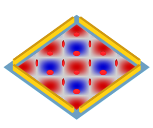
The time-averaged mean dynamics of RBCs driven by two orthogonal ultrasonic standing waves in a viscous fluid medium is investigated. The RBC is composed of a membrane enclosing an homogeneous fluid. It is assumed that the RBC can be represented as an oblate ellipsoid of a prescribed shape that never changes during the motion. Thus, the present work is valid when the RBC deformation remains small. Nevertheless, the membrane of the cell is allowed to circulate around the fixed ellipsoidal shape. The consideration of an oblate ellipsoid shape facilitates theoretical modelling and can well reproduce the dynamic behaviour of real biconcave erythrocytes in fluid experiments (Abkarian et al. Reference Abkarian, Faivre and Viallat2007). Two-dimensional ultrasonic standing waves are generated by the oscillation of two pairs of orthogonal piezoelectric transducers (PZTs), as shown in figure 1(a). When the two-dimensional standing waves are established, the cells are subjected to an acoustic radiation force, trapping the cells in the grid-like acoustic pressure nodes. Due to the presence of cavity/channel walls, boundary-driven Rayleigh streaming is generated (Hamilton, Ilinskii & Zabolotskaya Reference Hamilton, Ilinskii and Zabolotskaya2003). This streaming can influence trapping stability and cell dynamics in a cell size dependent manner. The influence is expected to be relatively small due to the large size of RBCs (Muller et al. Reference Muller, Barnkob, Jensen and Bruus2012). Furthermore, the Rayleigh streaming can be suppressed by a shape-optimized cavity/channel (Bach & Bruus Reference Bach and Bruus2020). Therefore, the boundary-driven Rayleigh streaming is neglected in our analysis.

Figure 1. Time-averaged mean dynamics of RBCs driven by two orthogonal ultrasonic standing waves. (a) Experimental set-up for generating two-dimensional standing waves. The background contour shows the acoustic pressure in (2.1) with phase difference  $\varphi = 0$, and the colour ranges from $- {p_{am}}$ (blue) to ${p_{am}}$ (red). (b) Coordinate systems and variables describing cell motion. Here, $(\hat{x},\hat{y},\hat{z})$ is the fixed coordinate frame, $(x,y,z)$ is the body coordinate frame, $\theta $ is the inclination angle describing cell rigid tumbling and $\phi $ is the phase angle describing membrane tank treading.
As shown in figure 1(b), let  $(\hat{x},\hat{y},\hat{z})$ denote a fixed Cartesian coordinate system that never changes with time and is therefore referred to as a fixed frame. The incident wave is composed of two orthogonal ultrasonic standing waves with the same acoustic pressure amplitude ${p_{am}}$ and frequency f, and the phase difference between them is $\zeta $. In the fixed frame $(\hat{x},\hat{y},\hat{z})$, the incident wave is given by
 \begin{equation}{p^{in}} = \frac{{{p_{am}}}}{2}\textrm{[}\sin ({k^e}\hat{y}) + \sin ({k^e}\hat{z})\,{\textrm{e}^{\textrm{i}\zeta }}\textrm{]}\,{\textrm{e}^{\textrm{i}\omega t}} + \textrm{c}.\textrm{c}.,\end{equation}
where  ${k^e} = \omega /c_0^e$ is the acoustic wavenumber and $c_0^e$ is the sound speed in the external viscous fluid, $\omega = 2{\rm \pi} f$ is the angular frequency, $\textrm{i} = \sqrt { - 1} $ is the imaginary unit, and $\textrm{c}.\textrm{c}.$ represents the complex conjugate of the first two terms.
As shown in figure 1(b), let  $(x,y,z)$ denote another Cartesian coordinate system, whose axes are the principal axes of the ellipsoidal cell, hence the name body frame. In the body frame $(x,y,z)$, the surface of the ellipsoidal cell is defined as
 \begin{equation}{\left( {\frac{x}{{{a_x}}}} \right)^2} + {\left( {\frac{y}{{{a_y}}}} \right)^2} + {\left( {\frac{z}{{{a_z}}}} \right)^2} = 1,\end{equation}
where  ${a_x}$, ${a_y}$ and ${a_z}$ are the three semi-axes. Here, the $x$-axis coincides with the $\hat{x}$-axis, while the $y$- and $z$-axes are rotated by an angle $\theta $ relative to the $\hat{y}$- and $\hat{z}$-axes, respectively, as shown in figure 1(b). The inclination angle $\theta $ describes the rotation of the ellipsoidal cell. Therefore, the inclination angle $\theta $ is a function of time, and $\dot{\theta } = \textrm{d}\theta /\textrm{d}t$ is the angular velocity of the ellipsoidal cell. In the following, the theoretical framework is conveniently formulated in the body frame $(x,y,z)$.
2.1. Mean dynamics of RBCs
The internal and external media of the cell are assumed to be compressible viscous fluids, whose fluid properties are characterized by shear viscosity  ${\eta ^{i,e}}$, bulk viscosity $\eta _b^{i,e}$, mass density $\rho _0^{i,e}$ and speed of sound $c_0^{i,e}$. The superscripts ‘ $i$’ and ‘ $e$’ relate to the internal and external media of the cell, respectively. Under high frequency acoustic excitation, the fluid dynamics is a combination of the fast time scale of ultrasound propagation $({\sim} 1\ {\rm \mu}{\rm s})$ and the slow time scale of mean dynamics $({\sim} 0.1\ \textrm{s)}$ for typical ultrasonic frequencies ~1 MHz. Here, the mean dynamics is actually time-averaged dynamics. During ultrasonic propagation on fast time scales, its nonlinear second-order terms produce a time-averaged mean stress, which drives the motion of cells on slow time scales. This process is called the mean dynamics of cells driven by ultrasonic waves.
The acoustic perturbation method based on the generalized Lagrangian formulation is employed to study the mean dynamics of cells driven by ultrasound (Nama, Huang & Costanzo Reference Nama, Huang and Costanzo2017). In contrast to the widely used fully Eulerian formulation (Bruus Reference Bruus2012), this formulation employs the perturbation expansion in the mean configuration, which is not disturbed by acoustic oscillation, thus having an exact definition of the boundary conditions at cell membranes. As shown in figure 2(a), the generalized Lagrangian formulation adopts separate definitions of the mean configuration and the deformed configuration. In the mean configuration, the particle motion follows the mean smooth trajectory, while in the deformed configuration, the particle motion follows an actual oscillating trajectory, which differs from the mean trajectory by acoustic oscillating displacement. The compressible Navier–Stokes equations in the deformed configuration are reformulated in the mean configuration, and then the perturbation expansion is applied to linearize the reformulated Navier–Stokes equations. Specifically, the fluid quantity g is decomposed as  $g = {g_0} + {g_1} + {g_2} + \cdots $, where ${g_0}$ is the zeroth-order (background) field, ${g_1}$ is the first-order field, and ${g_2}$ is the second-order field. The magnitude of the perturbation is characterized by the dimensionless acoustic Mach number $Ma = ||{\boldsymbol{v}_1}||/{c_0} \approx \textrm{1}{\textrm{0}^{ - 4}}$ with $||{\boldsymbol{v}_1}||$ being the amplitude of acoustic oscillating velocity, such that ${g_n} \propto M{a^n}$. Introducing the expansions of the reformulated Navier–Stokes equations and assuming zeroth-order fluid rest, one obtains two sets of governing equations: the first-order equations describe the ultrasound propagation and the time-averaged second-order equations describe the time-averaged mean dynamics (see Appendix A for details).

Figure 2. (a) Schematic of the material configuration  ${\mathrm{{\mathcal{B}}}_0}$ before acoustic excitation, the mean configuration $\mathrm{{\mathcal{B}}}$ of particle mean motion and the deformed configuration ${\mathrm{{\mathcal{B}}}_t}$ of particle actual motion. (b) Schematic of mean and actual trajectories with initial position $\boldsymbol{X}$. The difference between the mean position $\boldsymbol{x}$ and the actual position $\boldsymbol{y}$ of the particle is measured by the acoustic oscillation displacement $\boldsymbol{\xi }$.
In ultrasonic standing waves, there are viscous and thermal boundary layers around the cell, and the effects of viscosity and thermal conduction occur in the boundary layers. For most liquids, such as water, the thermal effect is relatively small because the ratio of thermal boundary layer thickness to viscous boundary layer thickness  ${\delta _t}/\delta \approx 0.3$ (Muller et al. Reference Muller, Barnkob, Jensen and Bruus2012). To simplify the theoretical treatment, the coupling between the thermal field and other fluid quantities is neglected. In such a case, the first-order equations for ultrasound propagation are expressed as
 \begin{equation}{\partial _t}{p_\textrm{1}} + {\rho _0}c_0^2\boldsymbol{\nabla }\boldsymbol{\cdot }{\boldsymbol{v}_\textrm{1}} = 0\quad \textrm{and}\quad {\rho _0}{\partial _t}{\boldsymbol{v}_\textrm{1}} - \boldsymbol{\nabla }\boldsymbol{\cdot }{\boldsymbol{P}_\textrm{1}} = \textbf{0},\end{equation}
with
 \begin{equation}{\boldsymbol{P}_\textrm{1}} =- {p_\textrm{1}}\boldsymbol{I} + \eta (\boldsymbol{\nabla }{\boldsymbol{v}_\textrm{1}} + \boldsymbol{\nabla }\boldsymbol{v}_\textrm{1}^T) + {\eta _b}(\boldsymbol{\nabla }\boldsymbol{\cdot }{\boldsymbol{v}_\textrm{1}})\boldsymbol{I}.\end{equation}
Here, all variables with subscript 1 correspond to first-order variables,  ${p_1}$ is the first-order acoustic pressure, ${\boldsymbol{v}_\textrm{1}}$ is the first-order acoustic oscillation velocity, ${\rho _0}$ is the fluid density, ${c_0}$ is the sound speed of the fluid, $\eta$ and ${\eta _b}$ are the shear the bulk viscosities of the fluid, respectively, and $\boldsymbol{I}$ is the identity matrix. In (2.3), the nonlinear convective acceleration term is neglected in the first-order acoustic wave equation because the second-order small variables are much smaller than the first-order variables.
The second-order equations for the time-averaged mean dynamics are expressed as
 \begin{equation}\boldsymbol{\nabla }\boldsymbol{\cdot }\langle {\boldsymbol{v}_2}\rangle = 0\quad \textrm{and}\quad \boldsymbol{\nabla }\boldsymbol{\cdot }\langle {\boldsymbol{P}_2}\rangle = \textbf{0},\end{equation}
with the second-order time-averaged Piola–Kirchhoff stress
 \begin{align} \langle {\boldsymbol{P}_2}\rangle & =- \langle {p_2}\rangle \boldsymbol{I} + \eta (\boldsymbol{\nabla }\langle {\boldsymbol{v}_2}\rangle + \boldsymbol{\nabla }{\langle {\boldsymbol{v}_2}\rangle ^T}) - \eta \langle (\boldsymbol{\nabla }{\boldsymbol{v}_1}\boldsymbol{\cdot }\boldsymbol{\nabla }\boldsymbol{\xi } + \boldsymbol{\nabla }{\boldsymbol{\xi }^T}\boldsymbol{\cdot }\boldsymbol{\nabla }\boldsymbol{v}_1^T)\rangle \notag\\ & \quad - {\eta _b}\langle \boldsymbol{\nabla }{\boldsymbol{\xi }^T}:\boldsymbol{\nabla }{\boldsymbol{v}_1}\rangle \boldsymbol{I} + \langle {\boldsymbol{P}_1}({\boldsymbol{v}_1}) \boldsymbol{\cdot} [(\boldsymbol{\nabla }\boldsymbol{\cdot }\boldsymbol{\xi })\boldsymbol{I} - \boldsymbol{\nabla }{\boldsymbol{\xi }^T}]\rangle . \end{align}
Here, all variables with subscript 2 correspond to second-order variables,  $\langle {p_2}\rangle $ is the time-averaged second-order pressure, $\langle {\boldsymbol{v}_2}\rangle $ is the time-averaged second-order velocity, $\boldsymbol{\xi } = {\partial _t}{\boldsymbol{v}_1}$ is the acoustic oscillation displacement and the operator $\langle \cdot \rangle$ represents the time average over an acoustic oscillating period. The first line in (2.6) represents the stress of incompressible fluid, while the second line of (2.6) consists of the products of two first-order acoustic quantities, representing the driving force for the time-averaged fluid flow and cell motion. It is worth noting that, in the context of this work, there is a time-averaged second-order flow that includes the acoustic streaming generated by the driving terms and the Stokes flows generated by the cell motion. For later use, (2.5) and (2.6) can be rewritten as
 \begin{equation}\boldsymbol{\nabla }\boldsymbol{\cdot }\langle {\boldsymbol{v}_2}\rangle = 0\quad \textrm{and}\quad \boldsymbol{\nabla }\boldsymbol{\cdot }[ - \langle {p_2}\rangle \boldsymbol{I} + \eta (\boldsymbol{\nabla }\langle {\boldsymbol{v}_2}\rangle + \boldsymbol{\nabla }{\langle {\boldsymbol{v}_2}\rangle ^T})]\textrm{ + }\boldsymbol{\nabla }\boldsymbol{\cdot }\mathrm{{\mathcal{B}}}({\boldsymbol{v}_1},\boldsymbol{\xi }) = \textbf{0},\end{equation}
with the tensor operator  $\mathrm{{\mathcal{B}}}$ defined as
 \begin{align}\mathrm{{\mathcal{B}}}({\boldsymbol{v}_1},\boldsymbol{\xi }) &=- \eta \langle (\boldsymbol{\nabla }{\boldsymbol{v}_1}\boldsymbol{\cdot }\boldsymbol{\nabla }\boldsymbol{\xi } + \boldsymbol{\nabla }{\boldsymbol{\xi }^T}\boldsymbol{\cdot }\boldsymbol{\nabla }\boldsymbol{v}_1^T)\rangle - {\eta _b}\langle \boldsymbol{\nabla }{\boldsymbol{\xi }^T}:\boldsymbol{\nabla }{\boldsymbol{v}_1}\rangle \boldsymbol{I}\notag\\ &\quad + \langle {\boldsymbol{P}_1}({\boldsymbol{v}_1})\boldsymbol{\cdot }[(\boldsymbol{\nabla }\boldsymbol{\cdot }\boldsymbol{\xi })\boldsymbol{I} - \boldsymbol{\nabla }{\boldsymbol{\xi }^T}]\rangle .\end{align}
In (2.8), by writing  ${\boldsymbol{P}_1}({\boldsymbol{v}_1})$, ${\boldsymbol{P}_1}$ is regarded as a function of ${\boldsymbol{v}_1}$ according to the first equation of (2.3).
To study the possible motion of the cell, the membrane is assumed to have a tank-treading motion. Let  $\boldsymbol{x}_s^0 = x_s^0{\boldsymbol{e}_x} + y_s^0{\boldsymbol{e}_y} + z_s^0{\boldsymbol{e}_z}$ represent the position vector of the material point on the membrane at the initial moment with $({\boldsymbol{e}_x},{\boldsymbol{e}_y},{\boldsymbol{e}_z})$ being the basis vector triad of the body frame. According to Keller & Skalak (Reference Keller and Skalak1982), the membrane elements are prescribed to circulate the cell surface relative to the body frame, and the relative velocity of a material point attached to the cell membrane relative to the body frame is derived as
 \begin{equation}{\boldsymbol{v}^m} = \dot{\phi }[ - ({a_y}/{a_z})z{\boldsymbol{e}_y} + ({a_z}/{a_y})y{\boldsymbol{e}_z}],\end{equation}
where  $\phi $ is the phase angle of the cell membrane (see figure 1b) and is a function of time t. It can be shown that ${\boldsymbol{v}^m}\boldsymbol{\cdot }\boldsymbol{n} = 0$, where $\boldsymbol{n}$ is the unit outward normal to the cell membrane. Thus, ${\boldsymbol{v}^m}$ is tangent to the cell membrane everywhere and represents the tank-treading motion. Finally, relative to the body frame, the velocity boundary conditions imposed on the external and internal fluids are
 \begin{gather}\langle \boldsymbol{v}_2^i\rangle = {\boldsymbol{v}^m}\quad \textrm{for}\;\boldsymbol{x} = {\boldsymbol{x}_s},\end{gather}
 \begin{gather}\langle \boldsymbol{v}_2^e\rangle = {\boldsymbol{v}^m}\quad \textrm{for}\;\boldsymbol{x} = {\boldsymbol{x}_s},\end{gather}
 \begin{gather}\langle \boldsymbol{v}_2^e\rangle =- \dot{\theta }{\boldsymbol{e}_x} \times \boldsymbol{x}\quad \textrm{for}\;|\boldsymbol{x}|\to \infty .\end{gather}
Recall that the equations are formulated in the body frame, and the far field flow condition (2.12) is due to the cell rigid tumbling motion. Moreover, the velocity of the material point attached to the membrane relative to the fixed frame is introduced as
 \begin{equation}{\boldsymbol{v}_s} = \boldsymbol{v}_s^{tt} + \boldsymbol{v}_s^{tu}.\end{equation}
Here,  ${\boldsymbol{v}_s}$ describes the synthetic motion of the membrane tank-treading motion $\boldsymbol{v}_s^{tt}$ and the cell rigid tumbling $\boldsymbol{v}_s^{tu} = \dot{\theta }{\boldsymbol{e}_x} \times {\boldsymbol{x}_s}$.
The time-averaged flow field can be obtained by successively solving the acoustic equation (2.3) with the incident wave in (2.1), and the time-averaged dynamic equation (2.7) together with the velocity boundary conditions (2.10)–(2.12). Since (2.7) has the structure of the Stokes equations and is linear with respect to the unknown variables  $(\langle {\boldsymbol{v}_2}\rangle ,\langle {p_2}\rangle )$, the solution to the time-averaged second-order flow field can be obtained by superposition of three ‘Stokes flow’ components
 \begin{equation}\langle {\boldsymbol{v}_2}\rangle = \langle \boldsymbol{v}_2^{ac}\rangle + \langle \boldsymbol{v}_2^{tu}\rangle + \langle \boldsymbol{v}_2^{tt}\rangle ,\end{equation}
where  $\langle \boldsymbol{v}_2^{ac}\rangle$ represents the ‘Stokes flow’ (i.e. acoustic streaming) generated by the acoustic dissipation in the viscous fluid, $\langle \boldsymbol{v}_2^{tu}\rangle$ represents the ‘Stokes flow’ generated by the rigid tumbling of the cell, and $\langle \boldsymbol{v}_2^{tt}\rangle$ represents the ‘Stokes flow’ generated by the tank treading of the cell membrane. Specifically, the acoustic streaming $\langle \boldsymbol{v}_2^{ac}\rangle$ is driven by the body force $\boldsymbol{\nabla }\boldsymbol{\cdot }\mathrm{{\mathcal{B}}}({\boldsymbol{v}_1},\boldsymbol{\xi })$ in (2.7) and is calculated by successively solving equations (2.3) and (2.7) independently of any second-order velocity excitation at the boundaries (i.e. $\dot{\theta } = \dot{\phi } = 0$, or equivalently, $\langle {\boldsymbol{v}^{ac}}\rangle = \textbf{0}$ in velocity boundary conditions (2.10)–(2.12)). Since the first-order acoustic oscillation velocity depends linearly on the input acoustic pressure amplitude, the second-order acoustic streaming velocity depends quadratically on the input acoustic pressure amplitude, i.e. $\langle \boldsymbol{v}_2^{ac}\rangle \propto p_{am}^2$. The ‘Stokes flows’ $\langle \boldsymbol{v}_2^{tu}\rangle$ and $\langle \boldsymbol{v}_2^{tt}\rangle$ are obtained by solving the Stokes equations (i.e. (2.7) without acoustic excitation) for different velocity boundary conditions: $\langle \boldsymbol{v}_2^{tu}\rangle \propto \dot{\theta }$ driven by velocity boundary condition (2.12) and $\langle \boldsymbol{v}_2^{tt}\rangle \propto \dot{\phi }$ driven by velocity boundary conditions (2.10) and (2.11).
Finally, the traction jump across the cell membrane can be obtained from the total time-averaged stress as
 \begin{equation}\boldsymbol{f} = (\langle \boldsymbol{P}_2^e\rangle - \langle \boldsymbol{P}_2^i\rangle )\boldsymbol{\cdot }\boldsymbol{n}.\end{equation}
Similar to the flow, the fluid traction jump can be extended to
 \begin{equation}\boldsymbol{f} = {\boldsymbol{f}^{ac}} + {\boldsymbol{f}^{tu}} + {\boldsymbol{f}^{tt}},\end{equation}
where  ${\boldsymbol{f}^{ac}}$, ${\boldsymbol{f}^{tu}}$ and ${\boldsymbol{f}^{tt}}$ are membrane tractions contributed by the flows $\langle \boldsymbol{v}_2^{ac}\rangle$, $\langle \boldsymbol{v}_2^{tu}\rangle$ and $\langle \boldsymbol{v}_2^{tt}\rangle$, respectively.
2.2. Acoustic streaming flow
The acoustic streaming flow  $\langle \boldsymbol{v}_2^{ac}\rangle$ around a fixed rigid ellipsoid membrane tilted at an angle $\theta $ can be obtained by directly solving the acoustic equation (2.3) with the incident wave in (2.1) and the time-averaged dynamic equation (2.5), similar to the work by Hahn et al. (Reference Hahn, Lamprecht and Dual2016). The phase difference $\zeta$ and inclination angle $\theta $ are implicitly included in the solution. Furthermore, in this work, an acoustic decomposition technique based on the superposition principle is used to obtain the acoustic streaming flow $\langle \boldsymbol{v}_2^{ac}\rangle$. As we will see, by using the acoustic decomposition technique, the phase difference $\zeta$ and inclination angle $\theta $ are separated from the acoustic streaming flow $\langle \boldsymbol{v}_2^{ac}\rangle$. This makes the acoustic decomposition technique more suitable for incorporation into the theoretical model of Keller & Skalak (Reference Keller and Skalak1982) for the analysis of cell dynamics. In addition, the acoustic decomposition technique provides insight into the underlying physical effects compared with directly solving the acoustic streaming flow $\langle \boldsymbol{v}_2^{ac}\rangle$.
The solution of the acoustic streaming flow  $\langle \boldsymbol{v}_2^{ac}\rangle$ is formulated in the body frame. Considering that the wavelength is much larger than the size of the cell, the input acoustic pressure in (2.1) can be approximately expressed by Taylor series expansion as
 \begin{equation}{p^{in}} \approx \frac{{{p_{am}}}}{2}\textrm{(}{k^e}\hat{y} + {k^e}\hat{z}\,{\textrm{e}^{\textrm{i}\zeta }}\textrm{)}\,{\textrm{e}^{\textrm{i}\omega t}} + \textrm{c}.\textrm{c}.\end{equation}
Rewriting equation (2.17) in the body frame, one obtains
 \begin{equation}{p^{in}} \approx \frac{{{p_{am}}}}{2}\textrm{[(}\cos \theta + {\textrm{e}^{\textrm{i}\zeta }}\sin \theta \textrm{)}{k^e}y + ({\textrm{e}^{\textrm{i}\zeta }}\cos \theta - \sin \theta ){k^e}z\textrm{]}\,{\textrm{e}^{\textrm{i}\omega t}} + \textrm{c}.\textrm{c}.\end{equation}
For the incident wave with vanishing viscous mode, the second equation of (2.3) becomes  ${\rho _0}{\partial _t}{\boldsymbol{v}_1} =- \boldsymbol{\nabla }\boldsymbol{\cdot }{p_1}$. Thus, the corresponding acoustic oscillation velocity is
 \begin{equation}{\boldsymbol{v}^{in}} \approx \frac{{{v_{am}}}}{2}\textrm{[}(\cos \theta + {\textrm{e}^{\textrm{i}\zeta }}\sin \theta ){\boldsymbol{e}_y} + ({\textrm{e}^{\textrm{i}\zeta }}\cos \theta - \sin \theta ){\boldsymbol{e}_z}\textrm{]}\,{\textrm{e}^{\textrm{i}\omega t}} + \textrm{c}.\textrm{c}.,\end{equation}
where  ${v_{am}} = {p_{am}}/(\textrm{i}\rho _0^ec_0^e)$ is the amplitude of the acoustic particle velocity. The solution to the acoustic equation (2.3) must match with the input acoustic excitation far from the cell (for $(x,y,z) \to \infty $).
Subjected to the acoustic excitation expressed by (2.18) and (2.19), the solution to the acoustic equations (2.3) can be assumed as
 \begin{equation}{\boldsymbol{v}_1} = {\tilde{p}_{am}}[\textrm{(}\cos \theta + {\textrm{e}^{\textrm{i}\zeta }}\sin \theta \textrm{)}\,{\textrm{e}^{\textrm{i}\omega t}}{\boldsymbol{v}_T} + ({\textrm{e}^{\textrm{i}\zeta }}\cos \theta - \sin \theta )\,{\textrm{e}^{\textrm{i}\omega t}}{\boldsymbol{v}_A}] + \textrm{c}.\textrm{c}.,\end{equation}
where  ${\tilde{p}_{am}} = {p_{am}}/{p_0}$ is the normalized acoustic pressure amplitude with the reference pressure ${p_0} = 1\ \textrm{MPa}$. Here, ${\boldsymbol{v}_T}$ is the one-dimensional standing wave response to the transverse acoustic excitation along the $y$-direction, while ${\boldsymbol{v}_A}$ is the one-dimensional standing wave response to the axial acoustic excitation along the $z$-direction. The subscripts ‘T’ and ‘A’ correspond to the transverse and axial acoustic excitations with respect to the cell, respectively. The linear superposition of these components constitutes the general solution. The component ${\boldsymbol{v}_T}$ is the solution of the following linear system and associated boundary conditions:
 \begin{equation}(\textrm{i}\omega ){p_T} + {\rho _0}c_0^2\boldsymbol{\nabla }\boldsymbol{\cdot }{\boldsymbol{v}_T} = 0\quad \textrm{and}\quad (\textrm{i}\omega ){\rho _0}{\boldsymbol{v}_T} - \boldsymbol{\nabla }\boldsymbol{\cdot }{\boldsymbol{P}_T} = \textbf{0},\end{equation}
with
 \begin{equation}{p_T} = {p_0}\frac{{{k^e}y}}{2}\quad \textrm{and}\quad {\boldsymbol{v}_T} = \frac{{{p_0}}}{{2\textrm{i}\rho _0^ec_0^e}}{\boldsymbol{e}_y}\ \textrm{as}\ (x,y,z) \to \infty .\end{equation}
Similarly, the component  ${\boldsymbol{v}_A}$ obeys
 \begin{equation}(\textrm{i}\omega ){p_A} + {\rho _0}c_0^2\boldsymbol{\nabla }\boldsymbol{\cdot }{\boldsymbol{v}_A} = 0\quad \textrm{and}\quad (\textrm{i}\omega ){\rho _0}{\boldsymbol{v}_A} - \boldsymbol{\nabla }\boldsymbol{\cdot }{\boldsymbol{P}_A} = \textbf{0},\end{equation}
with
 \begin{equation}{p_A} = {p_0}\frac{{{k^e}z}}{2}\quad \textrm{and}\quad {\boldsymbol{v}_A} = \frac{{{p_0}}}{{2\textrm{i}\rho _0^ec_0^e}}{\boldsymbol{e}_z}\ \textrm{as}\ (x,y,z) \to \infty .\end{equation}
 The solution of the time-averaged dynamic problem is obtained by substituting the acoustic solution (2.20) into the time-averaged dynamic equation (2.5). Since the time-averaged dynamic equation (2.5) is linear, the solution of  $\langle \boldsymbol{v}_2^{ac}\rangle$ can be assumed to be the sum of the solution components resulting from different terms in the expansion of $\mathrm{{\mathcal{B}}}({\boldsymbol{v}_1},\boldsymbol{\xi })$ as given in (B3) (see Appendix B). Formally, the solution of $\langle \boldsymbol{v}_2^{ac}\rangle$ can be expressed in the form
 \begin{align}\langle \boldsymbol{v}_2^{ac}\rangle & = (1 + \sin 2\theta \cos \zeta )\tilde{p}_{am}^2{\boldsymbol{v}_{TT}} + (1 - \sin 2\theta \cos \zeta )\tilde{p}_{am}^2{\boldsymbol{v}_{AA}}\notag\\ & \quad + \cos 2\theta \cos \zeta \tilde{p}_{am}^2\boldsymbol{v}_{AT}^0 + \sin \zeta \tilde{p}_{am}^2\boldsymbol{v}_{AT}^{{\rm \pi} /2}. \end{align}
The terms  ${\boldsymbol{v}_{TT}}$, ${\boldsymbol{v}_{AA}}$, $\boldsymbol{v}_{AT}^0$ and $\boldsymbol{v}_{AT}^{{\rm \pi} /2}$ are the solution components from the different contributions to the acoustic streaming. These terms depend only on the geometry of the cell and on the visco-acoustic properties (density, sound speed and viscosity) of the internal and external fluids. Specifically, in the first row of (2.25), the term ${\boldsymbol{v}_{TT}}$ corresponds to the nonlinear interaction of the acoustic response ${\boldsymbol{v}_T}$ with itself, and similarly, the term ${\boldsymbol{v}_{AA}}$ corresponds to the nonlinear interaction of the acoustic response ${\boldsymbol{v}_A}$ with itself. They are the solutions of the following linear problems:
 \begin{gather}\boldsymbol{\nabla
}\boldsymbol{\cdot }{\boldsymbol{v}_{TT}} = 0\quad
\textrm{and}\quad \begin{array}{*{20}{@{}l@{}}}\boldsymbol{\nabla }\boldsymbol{\cdot }[
- {p_{TT}}\boldsymbol{I} + \eta (\boldsymbol{\nabla
}{\boldsymbol{v}_{TT}} + \boldsymbol{\nabla
}\boldsymbol{v}_{TT}^T)]\\ \quad +\, \boldsymbol{\nabla
}\boldsymbol{\cdot
}[\mathrm{{\mathcal{B}}}({\boldsymbol{v}_T},\boldsymbol{\xi
}_T^ \ast ) + \mathrm{{\mathcal{B}}}(\boldsymbol{v}_T^ \ast
,{\boldsymbol{\xi }_T})] =
\textbf{0}
\end{array},\end{gather}
\begin{gather}\boldsymbol{\nabla
}\boldsymbol{\cdot }{\boldsymbol{v}_{TT}} = 0\quad
\textrm{and}\quad \begin{array}{*{20}{@{}l@{}}}\boldsymbol{\nabla }\boldsymbol{\cdot }[
- {p_{TT}}\boldsymbol{I} + \eta (\boldsymbol{\nabla
}{\boldsymbol{v}_{TT}} + \boldsymbol{\nabla
}\boldsymbol{v}_{TT}^T)]\\ \quad +\, \boldsymbol{\nabla
}\boldsymbol{\cdot
}[\mathrm{{\mathcal{B}}}({\boldsymbol{v}_T},\boldsymbol{\xi
}_T^ \ast ) + \mathrm{{\mathcal{B}}}(\boldsymbol{v}_T^ \ast
,{\boldsymbol{\xi }_T})] =
\textbf{0}
\end{array},\end{gather} \begin{gather}\boldsymbol{\nabla
}\boldsymbol{\cdot }{\boldsymbol{v}_{AA}} = 0\quad
\textrm{and}\quad \begin{array}{*{20}{@{}l@{}}}\boldsymbol{\nabla }\boldsymbol{\cdot }[
- {p_{AA}}\boldsymbol{I} + \eta (\boldsymbol{\nabla
}{\boldsymbol{v}_{AA}} + \boldsymbol{\nabla
}\boldsymbol{v}_{AA}^T)]\\ \quad +\, \boldsymbol{\nabla
}\boldsymbol{\cdot
}[\mathrm{{\mathcal{B}}}({\boldsymbol{v}_A},\boldsymbol{\xi
}_A^ \ast ) + \mathrm{{\mathcal{B}}}(\boldsymbol{v}_A^ \ast
,{\boldsymbol{\xi }_A})] =
\textbf{0}
\end{array},\end{gather}
\begin{gather}\boldsymbol{\nabla
}\boldsymbol{\cdot }{\boldsymbol{v}_{AA}} = 0\quad
\textrm{and}\quad \begin{array}{*{20}{@{}l@{}}}\boldsymbol{\nabla }\boldsymbol{\cdot }[
- {p_{AA}}\boldsymbol{I} + \eta (\boldsymbol{\nabla
}{\boldsymbol{v}_{AA}} + \boldsymbol{\nabla
}\boldsymbol{v}_{AA}^T)]\\ \quad +\, \boldsymbol{\nabla
}\boldsymbol{\cdot
}[\mathrm{{\mathcal{B}}}({\boldsymbol{v}_A},\boldsymbol{\xi
}_A^ \ast ) + \mathrm{{\mathcal{B}}}(\boldsymbol{v}_A^ \ast
,{\boldsymbol{\xi }_A})] =
\textbf{0}
\end{array},\end{gather}
where the asterisk indicates complex conjugate. Physically,  ${\boldsymbol{v}_{TT}}$ and ${\boldsymbol{v}_{AA}}$ can be understood as acoustic streaming flow driven by a one-dimensional standing wave propagating in the $y$-direction and $z$-direction, respectively. The terms $\boldsymbol{v}_{AT}^0$ and $\boldsymbol{v}_{AT}^{{\rm \pi} /2}$ in the second line of (2.25) correspond to the nonlinear interaction between the acoustic response ${\boldsymbol{v}_T}$ and the acoustic response ${\boldsymbol{v}_A}$. They are the solutions of the following linear problem:
 \begin{equation}\boldsymbol{\nabla
}\boldsymbol{\cdot }\boldsymbol{v}_{AT}^Z = 0\quad
\textrm{and}\quad \begin{array}{*{20}{@{}l@{}}}
{\boldsymbol{\nabla }\boldsymbol{\cdot }[ -
p_{AT}^Z\boldsymbol{I} + \eta (\boldsymbol{\nabla
}\boldsymbol{v}_{AT}^Z + \boldsymbol{\nabla }{\bf
(}\boldsymbol{v}_{AT}^Z{{\bf )}^T})] + \boldsymbol{\nabla
}\boldsymbol{\cdot
}[\mathrm{{\mathcal{B}}}({\boldsymbol{v}_T},{{({\textrm{e}^{\textrm{i}Z}}{\boldsymbol{\xi
}_A})}^ \ast })}\\ {\quad +\,
\mathrm{{\mathcal{B}}}({\textrm{e}^{\textrm{i}Z}}{\boldsymbol{v}_A},\boldsymbol{\xi
}_T^ \ast ) + \mathrm{{\mathcal{B}}}(\boldsymbol{v}_T^ \ast
,{\textrm{e}^{\textrm{i}Z}}{\boldsymbol{\xi }_A}) +
\mathrm{{\mathcal{B}}}({{({\textrm{e}^{\textrm{i}Z}}{\boldsymbol{v}_A})}^
\ast },{\boldsymbol{\xi }_T})] = \textbf{0}}
\end{array},\end{equation}
\begin{equation}\boldsymbol{\nabla
}\boldsymbol{\cdot }\boldsymbol{v}_{AT}^Z = 0\quad
\textrm{and}\quad \begin{array}{*{20}{@{}l@{}}}
{\boldsymbol{\nabla }\boldsymbol{\cdot }[ -
p_{AT}^Z\boldsymbol{I} + \eta (\boldsymbol{\nabla
}\boldsymbol{v}_{AT}^Z + \boldsymbol{\nabla }{\bf
(}\boldsymbol{v}_{AT}^Z{{\bf )}^T})] + \boldsymbol{\nabla
}\boldsymbol{\cdot
}[\mathrm{{\mathcal{B}}}({\boldsymbol{v}_T},{{({\textrm{e}^{\textrm{i}Z}}{\boldsymbol{\xi
}_A})}^ \ast })}\\ {\quad +\,
\mathrm{{\mathcal{B}}}({\textrm{e}^{\textrm{i}Z}}{\boldsymbol{v}_A},\boldsymbol{\xi
}_T^ \ast ) + \mathrm{{\mathcal{B}}}(\boldsymbol{v}_T^ \ast
,{\textrm{e}^{\textrm{i}Z}}{\boldsymbol{\xi }_A}) +
\mathrm{{\mathcal{B}}}({{({\textrm{e}^{\textrm{i}Z}}{\boldsymbol{v}_A})}^
\ast },{\boldsymbol{\xi }_T})] = \textbf{0}}
\end{array},\end{equation}
with  $\boldsymbol{v}_{AT}^0$ and $\boldsymbol{v}_{AT}^{{\rm \pi} /2}$ corresponding to $Z = \textrm{0}$ and $Z = {\rm \pi}/2$, respectively.
By successively solving the acoustic problem posed by (2.21)–(2.24) and the time-averaged dynamic problem posed by (2.26)–(2.28), one can obtain the acoustic streaming components  ${\boldsymbol{v}_{TT}}$, ${\boldsymbol{v}_{AA}}$, $\boldsymbol{v}_{AT}^0$ and $\boldsymbol{v}_{AT}^{{\rm \pi} /2}$ (see Appendix C for detailed numerical calculations). According to (2.25), the acoustic-induced traction jump ${\boldsymbol{f}^{ac}}$ can be expanded as
 \begin{align}
{\boldsymbol{f}^{ac}} & = (1 + \sin 2\theta \cos \zeta
)\tilde{p}_{am}^2{\,\boldsymbol{f}_{TT}} + (1 - \sin 2\theta
\cos \zeta )\tilde{p}_{am}^2{\,\boldsymbol{f}_{AA}}\notag\\ & \quad
+ \cos 2\theta \cos \zeta
\tilde{p}_{am}^2\,\boldsymbol{f}_{AT}^0 + \sin \zeta
\tilde{p}_{am}^2\,\boldsymbol{f}_{AT}^{{\rm \pi} /2},
\end{align}
\begin{align}
{\boldsymbol{f}^{ac}} & = (1 + \sin 2\theta \cos \zeta
)\tilde{p}_{am}^2{\,\boldsymbol{f}_{TT}} + (1 - \sin 2\theta
\cos \zeta )\tilde{p}_{am}^2{\,\boldsymbol{f}_{AA}}\notag\\ & \quad
+ \cos 2\theta \cos \zeta
\tilde{p}_{am}^2\,\boldsymbol{f}_{AT}^0 + \sin \zeta
\tilde{p}_{am}^2\,\boldsymbol{f}_{AT}^{{\rm \pi} /2},
\end{align}
where  ${\boldsymbol{f}_{TT}}$, ${\boldsymbol{f}_{AA}}$, $\boldsymbol{f}_{AT}^0$ and $\boldsymbol{f}_{AT}^{{\rm \pi} /2}$ are tractions contributed by the acoustic streaming components ${\boldsymbol{v}_{TT}}$, ${\boldsymbol{v}_{AA}}$, $\boldsymbol{v}_{AT}^0$ and $\boldsymbol{v}_{AT}^{{\rm \pi} /2}$, respectively. By using the acoustic decomposition technique, (2.29) isolates the influence of the phase difference $\zeta$ and inclination angle $\theta $ on the acoustic-induced traction jump ${\boldsymbol{f}^{ac}}$.
2.3. Torque balance and energy conservation for mean dynamics
The motion of the cell is completely characterized by the inclination angle  $\theta $ and the phase angle $\phi $, and their time evolution equations are established using the torque balance and energy conservation, respectively. The derivation of the time evolution equations follows the work by Keller & Skalak (Reference Keller and Skalak1982), who considered red blood cells in shear flow. Specifically, the Stokes flows ( $\langle \boldsymbol{v}_2^{tt}\rangle$ and $\langle \boldsymbol{v}_2^{tu}\rangle$) and their resulting membrane tractions ( $\,{\boldsymbol{f}^{tt}}$ and ${\boldsymbol{f}^{tu}}$) can be found in the work of Keller & Skalak (Reference Keller and Skalak1982) and references therein. The solutions of the acoustic streaming $\langle \boldsymbol{v}_2^{ac}\rangle$ and its resulting membrane traction ${\boldsymbol{f}^{ac}}$ have been formulated in § 2.2. With these solutions, the torque balance equation and the energy conservation equation for the red blood cell in a two-dimensional standing wave are given below.
The torque balance requires that the torque acting on the cell is zero, which can be expressed as
 \begin{equation}M = {\boldsymbol{e}_x}\boldsymbol{\cdot }\int_A {{\boldsymbol{x}_s} \times \boldsymbol{f}\,\textrm{d}A} = \int_A {(\kern 0.06em {y_s}\,{f_z} - {z_s}\,{f_y})\,\textrm{d}A} = 0,\end{equation}
where  ${f_y}$ and ${f_z}$ denote the y and z components of membrane traction $\boldsymbol{f}$, respectively, and A denotes the surface area of the cell membrane. According to the traction decomposition in (2.16), the torque balance can be expressed as
 \begin{equation}M = {M^{ac}} + {M^{tu}} + {M^{tt}} = 0,\end{equation}
where  ${M^{ac}}$, ${M^{tu}}$ and ${M^{tt}}$ are torques associated with the membrane tractions ${\boldsymbol{f}^{ac}}$, ${\boldsymbol{f}^{tu}}$ and ${\boldsymbol{f}^{tt}}$, respectively. The torques ${M^{tu}}$ and ${M^{tt}}$ are given by (see Appendix D for details)
 \begin{equation}{M^{tu}} =- C\dot{\theta }(a_y^2 + a_z^2)\quad \textrm{and}\quad {M^{tt}} =- 2C{a_y}{a_z}\dot{\phi },\end{equation}
with
 \begin{equation}C = \frac{{4V}}{{a_y^2{g_y} + a_z^2{g_z}}}.\end{equation}
Here, V is the volume of the cell, and  ${g_y}$ and ${g_z}$ are two geometric parameters of the ellipsoidal cell (see Appendix D for definitions). Due to the formulation of the acoustic streaming flow developed above, the corresponding torque ${M^{ac}}$ can be further expanded according to (2.29). Recalling that ${\boldsymbol{v}_{TT}}$ and ${\boldsymbol{v}_{AA}}$ are the acoustic streaming flow driven by the one-dimensional standing wave propagating in the $y$-direction and $z$-direction, respectively, the resulting membrane tractions ${\boldsymbol{f}_{TT}}$ and ${\boldsymbol{f}_{AA}}$ in (2.29) are symmetrical with respect to the three coordinate planes (i.e. the $xy$-, $yz$- and $xz$-planes), and therefore does not contribute to the torque acting on the cell. Consequently, the acoustic-induced torque is found to be
 \begin{equation}{M^{ac}} = \cos (2\theta )\cos \zeta \tilde{p}_{am}^2M_{AT}^0 + \sin \zeta \tilde{p}_{am}^2M_{AT}^{{\rm \pi} /2},\end{equation}
where  $M_{AT}^0$ and $M_{AT}^{{\rm \pi} /2}$ are the torques contributed by the membrane tractions $\boldsymbol{f}_{AT}^0$ and $\boldsymbol{f}_{AT}^{{\rm \pi} /2}$, respectively. The first term in (2.34) depends on the inclination angle with a factor $\cos (2\theta )$ and hence alternates between positive and negative with respect to $\theta$, while the second term is independent of $\theta$. These two torques were also qualitatively identified by Bernard et al. (Reference Bernard, Doinikov, Marmottant, Rabaud, Poulain and Thibault2017) based on the ideas of acoustic radiation torque and acoustic viscous torque, but their work did not give an accurate method to calculate the two torques. Substituting (2.32) and (2.34) into (2.31), the evolution equation of the inclination angle $\theta$ is
 \begin{equation}\dot{\theta } = \frac{{\cos \zeta \tilde{p}_{am}^2M_{AT}^0\cos (2\theta ) + \sin \zeta \tilde{p}_{am}^2M_{AT}^{{\rm \pi} /2} - 2C{a_y}{a_z}\dot{\phi }}}{{C(a_y^2 + a_z^2)}}.\end{equation}
In (2.35), the fluid viscosity appears explicitly in the parameter C originating from the torques  ${M^{tu}}$ and ${M^{tt}}$ generated by the Stokes flows, while appears implicitly in the torques $M_{AT}^0$ and $M_{AT}^{{\rm \pi} /2}$ generated by the acoustic streaming.
The energy conservation provides a constraint on the possible motion of the cell, that is, the rate of work done by the surrounding fluid is equal to the elastic power stored or dissipated in the membrane. By employing (2.13), the rate of work done by the surrounding fluid can be written as
 \begin{equation}\dot{W} = \int_A {{\boldsymbol{v}_s}\boldsymbol{\cdot }\boldsymbol{f}\,\textrm{d}A} = \int_A {\boldsymbol{v}_s^{tt}\boldsymbol{\cdot }\boldsymbol{f}\,\textrm{d}A} + \dot{\theta }{\boldsymbol{e}_x}\boldsymbol{\cdot }\int_A {{\boldsymbol{x}_s} \times \boldsymbol{f}\,\textrm{d}A} .\end{equation}
The last integral in (2.36) disappears according to the torque balance, so
 \begin{equation}\dot{W} = \int_A {\boldsymbol{v}_s^{tt}\boldsymbol{\cdot }\boldsymbol{f}\,\textrm{d}A} .\end{equation}
Substituting the membrane tank-treading velocity  $\boldsymbol{v}_s^{tt}$ given in (2.9) into (2.37), $\dot{W}$ can be expressed as
 \begin{equation}\dot{W} = \dot{\phi }W\quad \textrm{with}\;W = \int_A {\left( {\frac{{{a_z}}}{{{a_y}}}{y_s}{\,f_z} - \frac{{{a_y}}}{{{a_z}}}{z_s}{\,f_y}} \right)\,\textrm{d}A} .\end{equation}
Similar to the decomposition of the torque in (2.31), the work can be decomposed as
 \begin{equation}W = {W^{ac}} + {W^{tu}} + {W^{tt}},\end{equation}
where  ${\dot{W}^{ac}}$, ${\dot{W}^{tu}}$ and ${\dot{W}^{tt}}$ are the rates of work associated with the membrane tractions ${\boldsymbol{f}^{ac}}$, ${\boldsymbol{f}^{tu}}$ and ${\boldsymbol{f}^{tt}}$, respectively. The works ${W^{tu}}$ and ${W^{tt}}$ are given by (see Appendix D for details)
 \begin{equation}{\dot{W}^{tu}} =- 2{a_y}{a_z}C\dot{\theta }\quad \textrm{and}\quad {\dot{W}^{tt}} =- V{\eta ^i}{f_1}\dot{\phi } + V{\eta ^e}{f_2}\dot{\phi } - \frac{{4a_y^2a_z^2}}{{a_y^2 + a_z^2}}C\dot{\phi }.\end{equation}
Here,  ${f_1}$ and ${f_2}$ are two geometric parameters of the ellipsoidal cell (see Appendix D for definitions). Similar to the torque ${M^{ac}}$, the work ${W^{ac}}$ in (2.39) is expanded according to (2.29). Also, based on the symmetry of membrane tractions ${\boldsymbol{f}_{TT}}$ and ${\boldsymbol{f}_{AA}}$, it can be clarified that they do not contribute to the work of the membrane tank-treading motion. Since the acoustic streamings ${\boldsymbol{v}_{TT}}$ and ${\boldsymbol{v}_{AA}}$ represent the acoustic streaming flow driven by one-dimensional standing wave propagation, this reflects the factor that one-dimensional standing waves will not lead to the membrane tank-treading motion. Therefore, the work ${W^{ac}}$ can be expanded as
 \begin{equation}{W^{ac}} = \cos (2\theta )\cos \zeta \tilde{p}_{am}^2W_{AT}^0 + \sin \zeta \tilde{p}_{am}^2W_{AT}^{{\rm \pi} /2},\end{equation}
where  $W_{AT}^0$ and $W_{AT}^{{\rm \pi} /2}$ are understood as the works contributed by the terms $\boldsymbol{f}_{AT}^0$ and $\boldsymbol{f}_{AT}^{{\rm \pi} /2}$, respectively. However, the mechanical behaviour of the cell membrane is modelled by the Kelvin–Voigt viscoelastic model. The membrane stress is $\boldsymbol{\sigma } = 2{\eta ^m}\boldsymbol{D} + 2{\mu ^m}\boldsymbol{E}$, where ${\eta ^m}$ and ${\mu ^m}$ are the viscosity and shear modulus of the membrane, respectively. Here, the membrane viscosity ${\eta ^m}$ and shear modulus ${\mu ^m}$ are related to the two-dimensional membrane viscosity $\eta _{2D}^m$ and shear modulus $\mu _{2D}^m$ reported in other literature (e.g. Tsubota Reference Tsubota2021; Rezghi & Zhang Reference Rezghi and Zhang2022) by $\eta _{2D}^m = {\eta ^m}e$ and $\mu _{2D}^m = {\mu ^m}e$, respectively, where e is the membrane thickness. Here, $\boldsymbol{D}$ and $\boldsymbol{E}$ are the Eulerian strain rate tensor and the Eulerian strain tensor of the membrane, respectively. The elastic energy stored and dissipated in the membrane elements during tank treading is (Abkarian et al. Reference Abkarian, Faivre and Viallat2007)
 \begin{equation}\dot{E} = \int_\varOmega {\boldsymbol{\sigma }:\boldsymbol{D}\,\textrm{d}\varOmega } = \dot{\phi }\left[ {{f_1}{\eta^m}\dot{\phi } + \frac{1}{2}\dot{\phi }{f_1}{\mu^m}\sin (2\phi )} \right]\varOmega ,\end{equation}
where  $\varOmega = Ae$ is the membrane volume. It is important to note that ${\mu ^m}$ in (2.42) should be understood as the effective shear modulus, which contains the effect of the initial deformation from the unstressed shape to the elliptical shape of the cell at rest (Dupire et al. Reference Dupire, Abkarian and Viallat2015). Using energy conservation, which is translated as $\dot{W} = \dot{E}$, and employing (2.35) and (2.39)–(2.42), the evolution equation for the phase angle $\phi$ is
 \begin{align}\dot{\phi } = \frac{{\cos \zeta \tilde{p}_{am}^2(W_{AT}^0 - {f_3}M_{AT}^0)\cos (2\theta ) + \sin \zeta \tilde{p}_{am}^2(W_{AT}^{{\rm \pi} /2} - {f_3}M_{AT}^{{\rm \pi} /2}) - {\textstyle{1 \over 2}}\varOmega {\mu ^m}{f_1}\sin (2\phi )}}{{(V{\eta ^i}{f_1} - V{\eta ^e}{f_2} + \varOmega {\eta ^m}{f_1})}},\end{align}
where  ${f_3} = (2{a_y}{a_z})/(a_y^2 + a_z^2)$ is a geometric parameter of the ellipsoidal cell. In (2.43), the fluid viscosity appears explicitly in the denominator originating from the works ${W^{tu}}$ and ${W^{tt}}$ generated by the Stokes flows, while appears implicitly in the torques $M_{AT}^0$, $M_{AT}^{{\rm \pi} /2}$, $W_{AT}^0$ and $W_{AT}^{{\rm \pi} /2}$ generated by the acoustic streaming.
Equations (2.35) and (2.43) are the extension of the theoretical model describing RBC dynamics in shear flow by Keller & Skalak (Reference Keller and Skalak1982) to 2-D standing waves. Exactly, by replacing the torque and work due to 2-D standing waves with those due to shear flow in (2.35) and (2.43), one can recover the simplified theoretical model describing RBC dynamics in shear flow. After calculating  $M_{AT}^0$, $M_{AT}^{{\rm \pi} /2}$, $W_{AT}^0$ and $W_{AT}^{{\rm \pi} /2}$ (see Appendix C), the solutions of the cell motion are obtained by numerically solving the two coupled first-order ordinary differential equations (2.35) and (2.43) using the fourth-order Runge–Kutta method. The results are independent of the initial positions including the initial inclination angle ${\theta _0}$ and initial phase angle ${\phi _0}$, that is, changing the initial position will only produce a time shift in the results. Therefore, they are fixed to be $({\theta _0},{\phi _0}) = (0,0)$.
3. Results and discussion
The geometric parameters of the ellipsoidal RBC are considered to be consistent with previous studies:  ${a_1} = {a_2} = 4\ {\rm \mu}{\rm m}$, ${a_3} = 1.5\ {\rm \mu}{\rm m}$ and $e = 50\ \textrm{nm}$ (Abkarian et al. Reference Abkarian, Faivre and Viallat2007; Dupire et al. Reference Dupire, Abkarian and Viallat2015). The physical properties of the RBC cytoplasm are mass density $\rho _0^i = 1168\ \textrm{kg}\ {\textrm{m}^{ - 3}}$, sound speed $c_0^i = 1680\ \textrm{m}\ {\textrm{s}^{ - 1}}$ and shear viscosity ${\eta ^i} = 6 \times {10^{ - 3}}\ \textrm{Pa}\ \textrm{s}$ (Bagchi, Johnson & Popel Reference Bagchi, Johnson and Popel2005; Mishra, Hill & Glynne-Jones Reference Mishra, Hill and Glynne-Jones2014), while the physical properties of the surrounding fluid (set to water) are $\rho _0^e = 998\ \textrm{kg}\ {\textrm{m}^{ - 3}}$, $c_0^e = 1498\ \textrm{m}\ {\textrm{s}^{ - 1}}$ and ${\eta ^e} = 0.89 \times {10^{ - 3}}\ \textrm{Pa}\ \textrm{s}$. For simple fluids, the bulk viscosity is ${\eta _b} =- 2\eta /3$. The operating frequency is fixed at $f = 375\ \textrm{kHz}$ (Hahn et al. Reference Hahn, Lamprecht and Dual2016). In the typical acoustic microfluidic experiment, the range of phase difference is $\zeta = 0 \sim 0.5{\rm \pi} $, and the range of acoustic pressure amplitude is ${p_{am}} = 0 \sim 1\ \textrm{MPa}$ (Mishra et al. Reference Mishra, Hill and Glynne-Jones2014). Using these parameters, the acoustic streaming and RBC dynamics are calculated.
3.1. Flow structure of acoustic streaming
In this model, the dynamics of the RBC is driven by the torques and works of the acoustic streaming. To understand the response of RBCs in two-dimensional standing waves, the acoustic flow is first investigated. In (2.25), the acoustic streaming  $\langle \boldsymbol{v}_2^{ac}\rangle $ is expressed as a linear combination of four acoustic streaming components ${\boldsymbol{v}_{TT}}$, ${\boldsymbol{v}_{AA}}$, $\boldsymbol{v}_{AT}^0$ and $\boldsymbol{v}_{AT}^{{\rm \pi} /2}$. Figures 3(a–d) and 3(e–h) show the flow structures of the four acoustic streaming components and the corresponding time-averaged membrane traction forces generated by them, respectively. As mentioned earlier, ${\boldsymbol{v}_{TT}}$ and ${\boldsymbol{v}_{AA}}$ can be understood as the acoustic streamings driven by one-dimensional standing waves propagating along the $y$-axis and $z$-axis, respectively. Two classical streaming flow structures emerge (Chan et al. Reference Chan, Bhosale, Parthasarathy and Gazzola2022): ${\boldsymbol{v}_{TT}}$ falls into a bilayer regime outside the cell, characterized by an internal small vortex structure and an external flow extending to infinity, as shown in figure 3(a); ${\boldsymbol{v}_{AA}}$ falls into a monolayer regime as the inner layer thickness increases and eventually diverges, as shown in figure 3(b). Due to the symmetry of the acoustic streaming components ${\boldsymbol{v}_{TT}}$ and ${\boldsymbol{v}_{AA}}$ with respect to the $y$-axis and $z$-axis, the membrane traction forces ${\boldsymbol{f}_{TT}}$ and ${\boldsymbol{f}_{AA}}$ are also symmetrical with respect to the $y$-axis and $z$-axis, as shown in figures 3(e) and 3(f). Therefore, ${\boldsymbol{f}_{TT}}$ and ${\boldsymbol{f}_{AA}}$ make no contribution to the torque and work. In contrast, $\boldsymbol{v}_{AT}^0$ and $\boldsymbol{v}_{AT}^{{\rm \pi} /2}$ do not have this symmetry, as shown in figures 3(c) and 3(d), and the same is true for $\boldsymbol{f}_{AT}^0$ and $\boldsymbol{f}_{AT}^{{\rm \pi} /2}$, as shown in figures 3(g) and 3(h). The contributions of $\boldsymbol{f}_{AT}^0$ and $\boldsymbol{f}_{AT}^{{\rm \pi} /2}$ to the torque and work are therefore presented in table 1. As shown in figure 3(e–h), the maximum traction acting on the RBC membrane is ${\sim} 1\ \textrm{Pa}$, This level of traction in the 2-D standing wave considered in this work is comparable with that in the shear flow in the work of Abkarian et al. (Reference Abkarian, Faivre and Viallat2007). Considering that the RBC is a fixed ellipsoid but allows membrane tank treading in the theoretical model, good agreement between the theoretical results and experimental observation is achieved in the work of Abkarian et al. (Reference Abkarian, Faivre and Viallat2007). Therefore, it is believed that the present theoretical model, also considering the RBC as a fixed ellipsoid but allowing membrane tank treading, can give reasonable predictions of RBC dynamics.

Figure 3. (a–d) Time-averaged second-order velocity field and corresponding streamlines in the  $\hat{y}\hat{z}$ plane of the body frame. (e–f) Plots of the membrane traction: the arrow plots show the direction and relative magnitude of membrane traction; the line plots show the normal component ${f_n} = \boldsymbol{f}\boldsymbol{\cdot }\boldsymbol{n}$ and tangential component ${f_t} = \boldsymbol{f}\boldsymbol{\cdot }\boldsymbol{t}$ along the arclength s with $\boldsymbol{n}$ being the unit normal vector pointing outward the cell, and $\boldsymbol{t}$ being the unit tangential vector pointing clockwise. The first to fourth rows correspond to the four acoustic streaming components ${\boldsymbol{v}_{TT}}$, ${\boldsymbol{v}_{AA}}$, $\boldsymbol{v}_{AT}^0$ and $\boldsymbol{v}_{AT}^{{\rm \pi} /2}$, respectively. The red ellipse represents the RBC membrane.
Table 1. Values of torques and works.
To gain insight into the role of the acoustic streaming components  $\boldsymbol{v}_{AT}^0$ and $\boldsymbol{v}_{AT}^{{\rm \pi} /2}$, two special cases of phase differences $\xi = 0$ and ${\rm \pi} /2$ are considered. In view of (2.25), the total acoustic streamings in the two cases are
 \begin{gather}\langle \boldsymbol{v}_2^{ac}\rangle {|_{\xi = 0}} = (1 + \sin 2\theta ){\boldsymbol{v}_{TT}} + (1 - \sin 2\theta ){\boldsymbol{v}_{AA}} + \cos 2\theta \boldsymbol{v}_{AT}^0,\end{gather}
 \begin{gather}\langle \boldsymbol{v}_2^{ac}\rangle {|_{\xi = {\rm \pi}/2}} = {\boldsymbol{v}_{TT}} + {\boldsymbol{v}_{AA}} + \boldsymbol{v}_{AT}^{{\rm \pi} /2},\end{gather}
 where the acoustic pressure amplitude is set to  ${p_{am}} = 1\ \textrm{MPa}$. According to (3.1) and (3.2), $\boldsymbol{v}_{AT}^0$ and $\boldsymbol{v}_{AT}^{{\rm \pi} /2}$ can be understood as the asymmetric part of the acoustic streaming $\langle \boldsymbol{v}_2^{ac}\rangle {|_{\xi = 0}}$ and $\langle \boldsymbol{v}_2^{ac}\rangle {|_{\xi = {\rm \pi}/2}}$, respectively. At the phase difference $\xi = 0$, the two-dimensional standing wave approximates the propagating one-dimensional wave, as shown in figure 4(a). As the RBC is non-spherical, the acoustic streaming $\langle \boldsymbol{v}_2^{ac}\rangle {|_{\xi = 0}}$ depends on the inclination angle $\theta $. This is reflected by the different structures of $\langle \boldsymbol{v}_2^{ac}\rangle {|_{\xi = 0}}$ at the four different inclination angles $\theta = 0$, $- {\rm \pi}/4$, $- {\rm \pi}/2$ and $- 3{\rm \pi} /4$, as shown in figure 5(a–d). It can also be seen that $\langle \boldsymbol{v}_2^{ac}\rangle {|_{\xi = 0}}$ at $\theta =- {\rm \pi}/4$ and $- 3{\rm \pi} /4$ has the same structure as the acoustic streaming components ${\boldsymbol{v}_{AA}}$ and ${\boldsymbol{v}_{TT}}$, while its magnitude is twice those of ${\boldsymbol{v}_{AA}}$ and ${\boldsymbol{v}_{TT}}$, respectively. The dependence of $\langle \boldsymbol{v}_2^{ac}\rangle {|_{\xi = 0}}$ on the inclination angle $\theta $ is responsible for the factor $\cos 2\theta$ before $\boldsymbol{v}_{AT}^0$ in the acoustic streaming expression (2.25). At the phase difference $\xi = {\rm \pi}/2$, the two-dimensional standing wave approximates a vortex field, as shown in figure 4(b). This rotationally symmetrical acoustic field leads to the same acoustic streaming structure, regardless of the orientation of the RBC, as shown in figure 5(e–h). Thus, $\langle \boldsymbol{v}_2^{ac}\rangle {|_{\xi = {\rm \pi}/2}}$ is independent of the inclination angle $\theta $, which explains the fact that the factor before $\boldsymbol{v}_{AT}^{{\rm \pi} /2}$ in the acoustic streaming expression (2.25) is independent of the inclination angle $\theta $.

Figure 4. Contours of the root-mean-square acoustic pressure in the  $\hat{y}\hat{z}$ plane of the fixed frame for incident waves with different phase differences: (a) $\xi = 0$ and (b) $\xi = {\rm \pi}/2$. The acoustic pressure amplitude is ${p_{am}} = 1\ \textrm{MPa}$. The red ellipse represents the RBC membrane.

Figure 5. Acoustic streaming velocity and corresponding streamlines around the RBC in 2-D standing waves in the  $\hat{y}\hat{z}$ plane of the fixed frame for different phase differences: (a–d) $\xi = 0$ and (e–h) $\xi = {\rm \pi}/2$. The first to fourth rows correspond to the four inclination angles $\theta = 0$, $- {\rm \pi}/4$, $- {\rm \pi}/2$ and ${\rm \pi} /4$, respectively. The acoustic pressure amplitude is ${p_{am}} = 1\ \textrm{MPa}$. The red ellipse represents the RBC membrane.
3.2. Mean dynamics of red blood cells
The motion modes of the cell are controlled by two main conditions. First, (2.34) indicates that the cell is subjected to two types of acoustic-induced torques: the torque in the first term of (2.34) tends to align the major axis of the oblate cell at the specific angle  $\theta =- {\rm \pi}/4$, the torque in the second term tends to rotate the cell continuously. When the phase difference $\zeta $ increases from $0$ to ${\rm \pi} /2$, the magnitude of the latter torque gradually increases, and finally can exceed the former torque. Thus, the cell is aligned in a specific direction at small phase differences and tumbles at large phase differences (see the upper branch in figure 6). Second, the time-averaged fluid shear stress acting on the cell membrane, which is proportional to the square of the input acoustic pressure amplitude ${p_{am}}$, tends to circulate the membrane elements around the cell contour, while the membrane elastic restoring force tends to keep them in their initial positions. The latter is generally understood as an energy barrier and corresponds to the second term in (2.42). Let us consider the ${\rm \pi} /2$-circulation of the membrane around its contour: the membrane elements initially in the short axis region enter the long axis region, and vice versa. In this process, the cell membrane strains and stores elastic energy, which should be provided by the external work done by the time-averaged fluid shear stress. When ${p_{am}}$ is small, the shear stress is too small to overcome the energy barrier, and the membrane cannot tank tread. When ${p_{am}}$ is large, the shear stress can overcome the energy barrier, enabling the membrane to perform the tank-treading motion (see the lower branch in figure 6).

Figure 6. Schematic of the motion transition of an RBC, with the blue and green particles representing two material points attached to the cell membrane. The upper branch shows that the cell tumbles when the phase difference exceeds the critical phase difference, while the lower branch shows that the cell tank treads when the acoustic pressure amplitude exceeds the critical acoustic pressure amplitude.
More specifically, for small phase differences and small acoustic pressure amplitudes, the steady stationary state of the cell corresponds to steady solutions of (2.35) and (2.43). Letting the right-hand side of the equations equal to zero, the steady solutions of the inclination angle  ${\theta ^\# }$ and phase angle ${\phi ^\# }$ can be found as
 \begin{gather}{\theta ^\# } = \frac{1}{2}{\cos ^{ - 1}}\left( { - \frac{{M_{AT}^{{\rm \pi} /2}}}{{M_{AT}^0}}\tan \zeta } \right),\end{gather}
 \begin{gather}{\phi ^\# } = \frac{1}{2}{\sin ^{ - 1}}\left[ {\frac{{2\tilde{p}_{am}^2}}{{\varOmega {\mu^m}{f_1}}}\left( {W_{AT}^{{\rm \pi} /2} - W_{AT}^0\frac{{M_{AT}^{{\rm \pi} /2}}}{{M_{AT}^0}}} \right)\sin \zeta } \right].\end{gather}
The condition for the above solution is that the argument of the inverse trigonometric function should be in the range of [−1, 1], or equivalently,
 \begin{gather}\zeta < {\zeta ^c} \equiv {\tan ^{ - 1}}\left( {\frac{{M_{AT}^0}}{{M_{AT}^{{\rm \pi} /2}}}} \right),\end{gather}
 \begin{gather}{\tilde{p}_{am}} < \tilde{p}_{am}^c \equiv \sqrt {\frac{{\varOmega {\mu ^m}{f_1}}}{{2\sin \zeta }}{{\left( {W_{AT}^{{\rm \pi} /2} - W_{AT}^0\frac{{M_{AT}^{{\rm \pi} /2}}}{{M_{AT}^0}}} \right)}^{ - 1}}} .\end{gather}
Above the critical values of phase difference  ${\zeta ^c}$ and acoustic pressure amplitude $p_{am}^c$, steady solutions no longer exist, and tumbling or tank treading occurs, as shown in figure 6.
Then, a phase diagram is constructed for the dimensionless acoustic force  ${\tilde{P}^{ac}} = p_{am}^2\kappa _0^eR/(e{\mu ^m})$ and phase difference $\zeta $, as shown in figure 7(a). Here, the dimensionless acoustic force is introduced and defined as ${\tilde{P}^{ac}} = p_{am}^2\kappa _0^eR/(e{\mu ^m})$, where $\kappa _0^e = 1/[\rho _0^e{(c_0^e)^2}]$ is the adiabatic compressibility of the external fluid and $R = {({a_x}{a_y}{a_z})^{1/3}}$ is the effective radius of the cell. For the simplicity of the dimensionless formulation, the dimensionless acoustic force here is expressed as the ratio of the membrane traction force outside the cell generated by 2-D standing waves to the elastic force of the cell membrane, while the actual force that drives the deformation of the cell is the difference between the membrane traction force inside and outside the cell generated by 2-D standing waves. Due to the small difference in acoustic impedance of fluid inside and outside the cell, the difference in membrane traction force inside and outside the cell is also not significant, and the actual magnitude of this net membrane traction force is shown in figure 3. The effective shear modulus of the membrane is ${\mu ^m} = 0.5\ \textrm{Pa}$ and the viscosity of the membrane is ${\eta ^m} = 0\ \textrm{Pa}\ \textrm{s}$.

Figure 7. (a) Phase diagram of RBC motion in 2-D ultrasonic standing waves as a function of the dimensionless acoustic force  ${\tilde{P}^{ac}} = p_{am}^2\kappa _0^eR/(e{\mu ^m})$ and phase difference $\zeta $, showing four different regimes. The solid lines are the numerical solutions of (2.35) and (2.43), while the circles are the analytical solutions of (3.5) and (3.6). (b) Phase diagram of RBC motion in general linear flow as a function of the capillary number $Ca = G{\eta ^e}R/(e{\mu ^m})$ and parameter $\varsigma $ measuring the ratio of the strain rate to vorticity, also showing four different regimes. The mechanical properties of the cell membrane are: effective shear modulus ${\mu ^m} = 0.5\ \textrm{Pa}$ and surface viscosity ${\eta ^m} = 0\ \textrm{Pa}\ \textrm{s}$. (a) 2-D standing waves and (b) general linear flow.
As shown in figure 7(a), the above two conditions of (3.5) and (3.6) divide the phase space into four regions: in the steady stationary state for small  $\zeta $ and small ${\tilde{P}^{ac}}$, the inclination angle $\theta $ and phase angle $\phi $ asymptotically approach constant values ${\theta ^\# }$ and ${\phi ^\# }$, respectively (figure 8c); in the tank-treading motion state for small $\zeta $ and large ${\tilde{P}^{ac}}$, $\theta $ rotates and $\phi $ oscillates (figure 8d); in the tumbling motion state for large $\zeta $ and small ${\tilde{P}^{ac}}$, $\theta $ oscillates and $\phi $ rotates (figure 8a); in the intermittent rotation state for large $\zeta $ and large ${\tilde{P}^{ac}}$, $\theta $ and $\phi $ both rotates (figure 8b). The boundary of the steady stationary state is determined by the analytical expressions of (3.5) and (3.6), or the numerical solutions of (2.35) and (2.43). However, the boundaries between the other three motions need to be determined numerically because the motions of the inclination angle $\theta $ and phase angle $\phi $ are nonlinearly coupled in these states. At small dimensionless acoustic force ${\tilde{P}^{ac}}$, this phase diagram is consistent with the experimental observations of Bernard et al. (Reference Bernard, Doinikov, Marmottant, Rabaud, Poulain and Thibault2017). They investigated the effect of phase difference $\zeta $ on the motion of RBCs in a surface acoustic wave device and found that cell tumbling could only be observed when $\zeta $ was sufficiently large at the input acoustic pressure amplitude ${p_{am}} \approx 0.1\ \textrm{MPa}$. However, due to limited experimental working conditions, Bernard et al. (Reference Bernard, Doinikov, Marmottant, Rabaud, Poulain and Thibault2017) did not detect the tank-treading motion of the cells in their experiments. In contrast, at relatively large input acoustic pressure amplitude ${p_{am}} > 0.5\ \textrm{MPa}$, our theory and simulation have well predicted the tank-treading motion of the cells here, and have calculated the distributions of acoustic streaming and acoustic-induced stress in § 3.1, thus explaining the dynamic motion mechanism of cells at the level of the stress tensor. Furthermore, a similar phase diagram was observed in our previous 2-D finite element simulations, but the intermittent rotation regime has not yet been obtained (Liu & Xin Reference Liu and Xin2023b). This is the new finding of the present 3-D finite element simulation.

Figure 8. Typical temporal evolution of inclination angle  $\theta $ and phase angle $\phi $ in the four different regions in figure 7(a): (a) ${p_{am}} = 0.3\ \textrm{MPa}$ and $\zeta = 0.4{\rm \pi} $; (b) ${p_{am}} = 0.7\ \textrm{MPa}$ and $\zeta = 0.4{\rm \pi} $; (c) ${p_{am}} = 0.3\ \textrm{MPa}$ and $\zeta = 0.2{\rm \pi} $; and (d) ${p_{am}} = 0.9\ \textrm{MPa}$ and $\zeta = 0.29{\rm \pi} $. (a) Tumbling, (b) intermittent rotation, (c) steady stationary state and (d) tank treading.
For comparison, the RBC dynamics in a general linear flow beyond shear flow is presented. The velocity field of the flow is expressed as
 \begin{equation}{\boldsymbol{v}^g} = (s + w)\hat{z}{\hat{\boldsymbol{e}}_y} + (s - w)\hat{y}{\hat{\boldsymbol{e}}_z},\end{equation}
where s and w are the strain rate and vorticity, respectively. The theoretical model describing the dynamics of RBCs in general linear flow is given in Appendix D. Referring to the 2-D ultrasonic standing waves, s and w are rewritten as  $s = G{\cos ^2}\varsigma $ and $w = G{\sin ^2}\varsigma $, where $G = s + w$ measures the intensity of the flow and $\varsigma $ measures the ratio of the strain rate to vorticity.
A phase diagram is constructed for the capillary number  $Ca = G{\eta ^e}R/(e{\mu ^m})$ and parameter $\varsigma $ measuring the ratio of the strain rate to vorticity, as shown in figure 7(b). The phase diagrams in general linear flow and 2-D standing wave are globally similar, showing four dynamical regimes. The similarity can be analysed based on the two conditions governing the RBC dynamics mentioned above. For the first condition describing the competition between two types of torques, the two types of torque can be identified in both shear flow and 2-D standing wave. When $\zeta = \varsigma = 0$, (2.1) locally approximates a one-dimensional standing wave and (3.7) describes a purely extensional flow. The suspended cells are subjected to a pure extensional effect (Liu & Xin Reference Liu and Xin2023b), and the extensional effect tends to align RBCs in a specific direction. When $\zeta = \varsigma = {\rm \pi}/2$, (2.1) locally approximates a vortex acoustic field and (3.7) describes a purely rotational flow. The suspended cells are subjected to a pure rotational effect (Liu & Xin Reference Liu and Xin2023b), and the rotational effect tends to rotate the RBCs continuously. The $\varsigma $ and $\zeta $ control the ratio of the two types of torque in 2-D standing wave and general linear flow, respectively; in the same way, the larger the value of $\varsigma $ and $\zeta $, the larger the ratio of the torque tending to continuously rotate the RBCs to that tending to align the RBCs in a specific direction.
For the second condition describing the competition between the work done by the fluid shear stress and the energy barrier, the capillary number  $Ca$ and dimensionless acoustic force ${\tilde{P}^{ac}}$ control the ratio of the input work to the energy barrier in a 2-D standing wave and general linear flow, respectively; in the same way, the larger the value of $Ca$ and ${\tilde{P}^{ac}}$, the larger the ratio of the work to the energy barrier. As for the difference between 2-D ultrasonic standing waves and general linear flow, two separate regimes of intermittent rotational states are observed in 2-D ultrasonic standing waves, while only one regime is observed in general linear flow. This difference comes from the competition between the work done by the fluid shear stress and the energy barrier, here the fluid shear stress can be generated by cell tumbling and input energy (i.e. general linear flow and 2-D standing wave). In general linear flow, the work associated with the rotational part and the cell tumbling cancel each other out and only a regime of intermittent rotational state is observed, where the energy barrier is overcome by the work associated with the extensional part. In 2-D standing waves, the work associated with the rotational part and the cell tumbling are different. In one regime of the intermittent rotational state (small acoustic pressure amplitudes), the energy barrier is overcome by the work associated with the 2-D standing waves, while in the other regime of the intermittent rotational state (large acoustic pressure amplitudes), the energy barrier is overcome by the work associated with cell tumbling. It is worth noting that for the special case of $\varsigma = {\rm \pi}/4$, (3.7) describes the shear flow. As indicated by the dashed line in figure 7(b), only the tumbling motion and intermittent rotation are observed for shear flow due to the fixed ratio of the extension to rotation (Deschamps et al. Reference Deschamps, Kantsler, Segre and Steinberg2009).
As can be seen from (3.6), the transition between the steady stationary state and tank treading is related to the effective shear modulus of the membrane  ${\mu ^m}$. It can therefore be anticipated that the experimental values of the critical acoustic pressure amplitude fitted with (3.6) can be used to determine the effective shear modulus of cell membrane ${\mu^m}$. However, this transition is independent of the membrane viscosity ${\eta ^m}$, as the energy barrier of the membrane tank-treading motion is independent of the membrane viscosity. To assess the membrane viscosity, the dynamical parameters of tank-treading motion are analysed. Figure 9 shows the tank-treading frequency ${f^{tt}}$ (i.e. the reciprocal of the time for $2{\rm \pi} $-rotation of the phase angle) and the average inclination ${\theta ^m}$ (i.e. the average inclination angle during oscillation) versus the membrane viscosity ${\eta ^m}$, where the values of ${\eta ^m}$ cover the literature value of RBC membranes ranging as $0.7 \sim 2\ \textrm{Pa}\ \textrm{s}$ (Abkarian et al. Reference Abkarian, Faivre and Viallat2007). Figure 9 also shows the influence of cytoplasmic viscosity. The range of literature values for cytoplasmic viscosity is $5 \sim 55\ \textrm{mPa}\ \textrm{s}$. Four different values of cytoplasmic viscosity ${\eta ^i}$ are considered: 6, 12, 24 and $48\ \textrm{mPa}\ \textrm{s}$. Figure 9(a) shows that the tank-treading frequency ${f^{tt}}$ decreases with increasing membrane viscosity and increasing cytoplasmic viscosity. This is because the greater the viscosity of the cell membrane and cytoplasm, the greater the viscous resistance impeding the cell membrane tank-treading motion, and the slower the angular velocity or frequency of the cell tank-treading motion. It can also be observed from figure 9(a) that the four lines representing the different cytoplasmic viscosities tend to merge. Thus, at high membrane viscosities, the tank-treading frequency is almost independent of the cytoplasmic viscosity. Figure 9(b) shows that increasing membrane viscosity and increasing cytoplasmic viscosity align the cell closer to the inclination angle ${\theta ^\# }$ of RBCs with a rigid membrane, indicated by the dashed lines. This is because increasing membrane viscosity and increasing cytoplasmic viscosity stiffen the cell membrane.

Figure 9. (a) Tank-treading frequency  ${f^{tt}}$ and (b) average inclination ${\theta ^m}$ versus membrane viscosity for different cytoplasmic viscosity at the acoustic pressure amplitude ${p_{am}} = 0.8\ \textrm{MPa}$ and the phase difference $\zeta = 0.2{\rm \pi} $.
4. Concluding remarks
A computational model is developed to study the time-averaged dynamics of RBCs trapped in the acoustic pressure nodes of two orthogonal ultrasonic standing waves with phase difference. In the context of the generalized Lagrangian formulation, the time-averaged mean stress caused by acoustic nonlinear effect is obtained by the acoustic perturbation method. The cell is modelled as a viscoelastic membrane enclosing a homogeneous fluid, while simplifying its dynamics by constraining two degrees of freedom: the inclination angle of the ellipsoidal cell shape and the phase angle of the potential tank-treading motion of the cell membrane. Based on torque balance and energy conservation, the evolution equations of the inclination angle and the phase angle are derived, respectively.
In two-dimensional standing waves, RBCs have four different types of motion: the steady stationary state, tumbling motion, tank-treading motion and intermittent rotation, in which both inclination angle and phase angle rotate. The transition from the steady stationary state to tumbling motion is caused by the competition between two types of acoustic-induced torques: one tends to align the cell in a specific direction and the other tends to cause the cell to tumble. Consistent with experimental observations, the transition is found by increasing the phase difference until the latter torque overcomes the former. The tank-treading motion occurs when the acoustic-induced shear stresses overcome the energy barrier of the cell membrane. This requirement is met when the acoustic pressure amplitude is relatively large (larger than  $0.5\ \textrm{MPa}$) compared to those used for only rigid-body translational or rotational manipulation of cells (approximately $0.1\ \textrm{MPa}$), but still within the cell-friendly range. It is hoped that the present results will help guide future experimental work to control the time-averaged dynamics of RBCs with acoustic techniques, and further help to extract the viscoelastic properties of cell membranes by fitting experimental observations with the present computational model.
Fundings
This work was supported by the National Natural Science Foundation of China (52375122, 52075416 and 11772248), the Science Fund for Distinguished Young Scholars of Shaanxi Province (2023-JC-JQ-06) and the Fundamental Research Funds for the Central Universities (LX6J013).
Declaration of interest
The author reports no conflict of interest.
Appendix A. Acoustic perturbation method in the generalized Lagrangian formulation
The fluid hydrodynamics considered in this work is governed by the Navier–Stokes equations in the deformed configuration  ${\mathrm{{\mathcal{B}}}_t}$
 \begin{gather}{\dot{\rho }^{\# }} + {\rho ^{\# }}\boldsymbol{\nabla }\boldsymbol{\cdot }{\boldsymbol{v}^{\# }} = 0\ \textrm{in}\ {\mathrm{{\mathcal{B}}}_t},\end{gather}
 \begin{gather}{\rho ^\# }{\dot{\boldsymbol{v}}^\# } + \boldsymbol{\nabla }\boldsymbol{\cdot }{\boldsymbol{\sigma }^\# } = \textbf{0}\ \textrm{in}\ {\mathrm{{\mathcal{B}}}_t},\end{gather}
where  ${\rho ^\# }$ is the fluid density, ${\boldsymbol{v}^\# }$ is the fluid velocity and ${\boldsymbol{\sigma }^\# }$ is the Cauchy stress. The superscript $\# $ denotes the quantities defined in the deformed configuration ${\mathrm{{\mathcal{B}}}_t}$, which are functions of time t and position $\boldsymbol{y}$ (see figure 2a). Assuming the fluid is linear, viscous and compressible, the constitutive response function for the Cauchy stress is
 \begin{equation}{\boldsymbol{\sigma }^\# } =- {p^\# }({\rho ^\# })\boldsymbol{I} + \eta (\boldsymbol{\nabla }{\boldsymbol{v}^\# } + \boldsymbol{\nabla }{\boldsymbol{v}^\# }^T) + {\eta _b}(\boldsymbol{\nabla }\boldsymbol{\cdot }{\boldsymbol{v}^\# })\boldsymbol{I},\end{equation}
where  ${p^\# }$ is the fluid pressure, $\mu $ and ${\mu _b}$ are the shear and bulk viscosities, respectively. When the fluid is subjected to acoustic waves, the following linear relationship is assumed:
 \begin{equation}{p^\# } = c_0^2({\rho ^\# } - {\rho _0}),\end{equation}
where  ${c_0}$ and ${\rho _0}$ are constants that represent the sound speed and density of the fluid at rest.
The acoustic perturbation method in the generalized Lagrangian formulation developed by Nama et al. (Reference Nama, Huang and Costanzo2017) is briefly reviewed here. First, the Navier–Stokes equations are reformulated in the mean configuration. The field  ${g^\# }$ defined in the deformed configuration ${\mathrm{{\mathcal{B}}}_t}$ can be mapped onto the mean configuration $\mathrm{{\mathcal{B}}}$ according to the following definition:
 \begin{equation}g(\boldsymbol{x},t) = {g^\# }(\kern 0.06em\boldsymbol{y},t){|_{\boldsymbol{y} = \boldsymbol{x} + \boldsymbol{\xi }(\boldsymbol{x},t)}},\end{equation}
where g is a function of time t and position  $\boldsymbol{x}$ (see figure 2a). Using the above definition, (A1) and (A2) can be expressed in the mean configuration as
 \begin{gather}{\partial _t}\rho + \boldsymbol{F}_\xi ^{ - T}\boldsymbol{\cdot }\boldsymbol{\nabla }\rho \boldsymbol{\cdot }(\boldsymbol{v} - {\boldsymbol{v}_\xi }) + \rho \boldsymbol{F}_\xi ^{ - T}:\boldsymbol{\nabla }\boldsymbol{v} = 0\ \textrm{in}\ \mathrm{{\mathcal{B}}},\end{gather}
 \begin{gather}{J_\xi }\rho [{\partial _t}\boldsymbol{v} + \boldsymbol{\nabla }\boldsymbol{v}\boldsymbol{\cdot }\boldsymbol{F}_\xi ^{ - 1}\boldsymbol{\cdot }(\boldsymbol{v} - {\boldsymbol{v}_\xi })] - \boldsymbol{\nabla }\boldsymbol{\cdot }\boldsymbol{P} = \textbf{0}\ \textrm{in}\ \mathrm{{\mathcal{B}}},\end{gather}
where  ${\boldsymbol{F}_\xi } = \boldsymbol{\nabla }\boldsymbol{\xi }$ and ${J_\xi } = \det ({\boldsymbol{F}_\xi })$ are the gradient of acoustic oscillation displacement and its Jacobian determinant. In (A7), $\boldsymbol{P}$ is the Piola–Kirchhoff stress tensor (i.e. nominal stress tensor), representing the stress measured per unit area in the mean configuration, and is defined as
 \begin{equation}\boldsymbol{P} = {J_\xi }\boldsymbol{\sigma }\boldsymbol{\cdot }\boldsymbol{F}_\xi ^{ - T}.\end{equation}
Then, the acoustic perturbation method is applied to linearize (A6) and (A7). Subjected to acoustic waves, a tiny perturbation  ${\rho _1}$ in the fluid density and ${\boldsymbol{v}_1}$ in the fluid velocity are induced. The magnitude of the perturbation is characterized by the dimensionless acoustic Mach number
 \begin{equation}Ma = \frac{{{v_1}}}{{{c_0}}} = \frac{{{\rho _1}}}{{{\rho _0}}} \ll 1,\end{equation}
where  ${v_1} = |{\boldsymbol{v}_1}|$. In a typical acoustofluidic system $Ma \approx {10^{ - 4}}$, therefore, a perturbation expansion of fluid quantity g in order of Ma makes sense, $g = {g_0} + {g_1} + {g_2} + \cdots $, where ${g_n} \propto M{a^n}$. The expansions in fluid density $\rho $, pressure p and velocity $\boldsymbol{v}$ are given by
 \begin{gather}\rho = {\rho _0} + {\rho _1} + {\rho _2},\end{gather}
 \begin{gather}p = {p_0} + {p_1} + {p_2},\end{gather}
 \begin{gather}\boldsymbol{v} = {\boldsymbol{v}_1} + {\boldsymbol{v}_2},\end{gather}
where the numbers in the subscripts indicate the corresponding order. The system is considered to be initially at rest with velocity  ${\boldsymbol{v}_0} = \textbf{0}$, density ${\rho _0} = \textrm{const}\textrm{.}$ and pressure ${p_0} = \textrm{const}\textrm{.}$ before acoustic excitation. The first-order response $({\rho _1},{p_1},{\boldsymbol{v}_1})$ represents the first-order linear acoustic field, and the second-order response $({\rho _2},{p_2},{\boldsymbol{v}_2})$ represents the second-order nonlinear acoustic field.
Substituting (A10)–(A12) into (A6) and (A7), the first-order equations describing the acoustic wave propagation is obtained as
 \begin{gather}{\partial _t}{p_1} + {\rho _0}c_0^2\boldsymbol{\nabla }\boldsymbol{\cdot }{\boldsymbol{v}_1} = 0\ \textrm{in}\ \mathrm{{\mathcal{B}}},\end{gather}
 \begin{gather}{\rho _0}{\partial _t}{\boldsymbol{v}_1} + \boldsymbol{\nabla }\boldsymbol{\cdot }{\boldsymbol{P}_1} = 0\ \textrm{in}\ \mathrm{{\mathcal{B}}},\end{gather}
with the first-order Piola–Kirchhoff stress
 \begin{equation}{\boldsymbol{P}_1} =- {p_1}\boldsymbol{I} + \eta (\boldsymbol{\nabla }{\boldsymbol{v}_1} + \boldsymbol{\nabla }\boldsymbol{v}_1^T) + {\eta _b}(\boldsymbol{\nabla }\boldsymbol{\cdot }{\boldsymbol{v}_1})\boldsymbol{I}.\end{equation}
 The acoustofludic dynamics observed in the experiments occurs on a sub- $s$ time scale, which is much slower than the ultrasonic ${\rm \mu} \mathrm{s}$ time scale. The quantities in the acoustofludic dynamics are represented by the time-averaged operator $\langle \cdot \rangle$. The time-averaged second-order equations describing the acoustofludic dynamics response, are given by
 \begin{gather}\boldsymbol{\nabla }\boldsymbol{\cdot }\langle {\boldsymbol{v}_2}\rangle = 0\;\textrm{in}\ \mathrm{{\mathcal{B}}},\end{gather}
 \begin{gather}\boldsymbol{\nabla }\boldsymbol{\cdot }\langle {\boldsymbol{P}_2}\rangle = \textbf{0}\ \textrm{in}\ \mathrm{{\mathcal{B}}},\end{gather}
with the time-averaged second-order Piola-Kirchhoff stress
 \begin{align}\langle {\boldsymbol{P}_2}\rangle & =- \langle {p_2}\rangle \boldsymbol{I} + \eta (\boldsymbol{\nabla }\langle {\boldsymbol{v}_2}\rangle + \boldsymbol{\nabla }{\langle {\boldsymbol{v}_2}\rangle ^T}) - \eta \langle \boldsymbol{\nabla }{\boldsymbol{v}_1}\boldsymbol{\cdot }\boldsymbol{\nabla }\boldsymbol{\xi } + \boldsymbol{\nabla }{\boldsymbol{\xi }^T}\boldsymbol{\cdot }\boldsymbol{\nabla }\boldsymbol{v}_1^T\rangle \notag\\ & \quad - {\eta _b}\langle \boldsymbol{\nabla }{\boldsymbol{\xi }^T}:\boldsymbol{\nabla }{\boldsymbol{v}_1}\rangle \boldsymbol{I} + \langle {\boldsymbol{P}_1}\boldsymbol{\cdot }[(\boldsymbol{\nabla }\boldsymbol{\cdot }\boldsymbol{\xi })\boldsymbol{I} - \boldsymbol{\nabla }{\boldsymbol{\xi }^T}]\rangle . \end{align}
In acoustic streaming calculations, there is usually a Stokes drift term in addition to the Eulerian streaming flow field to account for the Lagrangian motion of particles. Here, since the Lagrangian acoustic perturbation method is used, the Lagrangian streaming flow can be obtained directly without the need to convert the Eulerian streaming flow to the Lagrangian streaming flow by using the Stokes drift. Essentially, the Lagrangian streaming flow we obtain actually consists of Eulerian streaming flow and the Stokes drift term.
Appendix B. Expansion of the nonlinear operator  $\mathrm{\mathcal{B}}({\boldsymbol{v}_1},\boldsymbol{\xi })$

The acoustic oscillation velocity  ${\boldsymbol{v}_1}$ given in (2.20) is expressed as
 \begin{align}{\boldsymbol{v}_1} & = (\cos \theta + {\textrm{e}^{\textrm{i}\zeta }}\sin \theta )\,{\textrm{e}^{\textrm{i}\omega t}}{\boldsymbol{v}_T} + ({\textrm{e}^{\textrm{i}\zeta }}\cos \theta - \sin \theta )\,{\textrm{e}^{\textrm{i}\omega t}}{\boldsymbol{v}_A}\notag\\ & \quad + (\cos \theta + {\textrm{e}^{ - \textrm{i}\zeta }}\sin \theta )\,{\textrm{e}^{ - \textrm{i}\omega t}}\boldsymbol{v}_T^ \ast+ ({\textrm{e}^{ - \textrm{i}\zeta }}\cos \theta - \sin \theta )\,{\textrm{e}^{ - \textrm{i}\omega t}}\boldsymbol{v}_A^ \ast , \end{align}
where the asterisk represents the complex conjugate. Correspondingly, the acoustic oscillating displacement  $\boldsymbol{\xi }$ is expressed as
 \begin{align}\boldsymbol{\xi } & = (\cos \theta + {\textrm{e}^{\textrm{i}\zeta }}\sin \theta )\,{\textrm{e}^{\textrm{i}\omega t}}{\boldsymbol{\xi }_T} + ({\textrm{e}^{\textrm{i}\zeta }}\cos \theta - \sin \theta )\,{\textrm{e}^{\textrm{i}\omega t}}{\boldsymbol{\xi }_A}\notag\\ & \quad + (\cos \theta + {\textrm{e}^{ - \textrm{i}\zeta }}\sin \theta )\,{\textrm{e}^{ - \textrm{i}\omega t}}\boldsymbol{\xi }_T^ \ast+ ({\textrm{e}^{ - \textrm{i}\zeta }}\cos \theta - \sin \theta )\,{\textrm{e}^{ - \textrm{i}\omega t}}\boldsymbol{\xi }_A^ \ast .\end{align}
Substituting (B1) and (B2) into  $\mathrm{{\mathcal{B}}}({\boldsymbol{v}_1},\boldsymbol{\xi })$, one obtains
 \begin{align}\mathrm{{\mathcal{B}}}({\boldsymbol{v}_1},\boldsymbol{\xi
}) & = \tilde{p}_{am}^2\mathrm{{\mathcal{B}}}\left(
{\begin{array}{*{20}{@{}c@{}}} {\left[ \begin{array}{@{}l@{}}
\textrm{(}\cos \theta + {\textrm{e}^{\textrm{i}\zeta }}\sin
\theta \textrm{)}\,{\textrm{e}^{\textrm{i}\omega
t}}{\boldsymbol{v}_T} + ({\textrm{e}^{\textrm{i}\zeta
}}\cos \theta - \sin \theta
)\,{\textrm{e}^{\textrm{i}\omega t}}{\boldsymbol{v}_A}\\
\quad +\, (\cos \theta + {\textrm{e}^{ - \textrm{i}\zeta
}}\sin \theta )\,{\textrm{e}^{ - \textrm{i}\omega
t}}\boldsymbol{v}_T^ \ast+ ({\textrm{e}^{ - \textrm{i}\zeta
}}\cos \theta - \sin \theta )\,{\textrm{e}^{ -
\textrm{i}\omega t}}\boldsymbol{v}_A^ \ast \end{array}
\right],}\\ {\left[ \begin{array}{@{}l@{}} \textrm{(}\cos \theta
+ {\textrm{e}^{\textrm{i}\zeta }}\sin \theta
\textrm{)}\,{\textrm{e}^{\textrm{i}\omega
t}}{\boldsymbol{\xi }_T} + ({\textrm{e}^{\textrm{i}\zeta
}}\cos \theta - \sin \theta
)\,{\textrm{e}^{\textrm{i}\omega t}}{\boldsymbol{\xi }_A}\\
\quad +\, (\cos \theta + {\textrm{e}^{ - \textrm{i}\zeta
}}\sin \theta )\,{\textrm{e}^{ - \textrm{i}\omega
t}}\boldsymbol{\xi }_T^ \ast+ ({\textrm{e}^{ -
\textrm{i}\zeta }}\cos \theta - \sin \theta
)\,{\textrm{e}^{ - \textrm{i}\omega t}}\boldsymbol{\xi }_A^
\ast \end{array} \right]} \end{array}} \right)\notag\\ & =
\tilde{p}_{am}^2\left\{ \begin{array}{@{}l@{}} (1 + \cos \zeta
\sin 2\theta
)[\mathrm{{\mathcal{B}}}({\boldsymbol{v}_T},\boldsymbol{\xi}_T^
\ast ) + \mathrm{{\mathcal{B}}}(\boldsymbol{v}_T^ \ast
,{\boldsymbol{\xi }_T})]\\ \quad + \,(1 - \cos \zeta \sin
2\theta
)[\mathrm{{\mathcal{B}}}({\boldsymbol{v}_A},\boldsymbol{\xi}_A^
\ast ) + \mathrm{{\mathcal{B}}}(\boldsymbol{v}_A^ \ast
,{\boldsymbol{\xi }_A})]\\ \quad + \cos \zeta \cos 2\theta
[\mathrm{{\mathcal{B}}}({\boldsymbol{v}_T},\boldsymbol{\xi}_A^
\ast ) +
\mathrm{{\mathcal{B}}}({\boldsymbol{v}_A},\boldsymbol{\xi}_T^
\ast ) + \mathrm{{\mathcal{B}}}(\boldsymbol{v}_T^ \ast
,{\boldsymbol{\xi}_A}) +
\mathrm{{\mathcal{B}}}(\boldsymbol{v}_A^ \ast
,{\boldsymbol{\xi }_T})]\\ \quad + \sin \zeta
[\mathrm{{\mathcal{B}}}({\boldsymbol{v}_T},{(\textrm{i}{\boldsymbol{\xi}_A})^
\ast }) +
\mathrm{{\mathcal{B}}}(\textrm{i}{\boldsymbol{v}_A},\boldsymbol{\xi}_T^
\ast ) + \mathrm{{\mathcal{B}}}(\boldsymbol{v}_T^ \ast
,\textrm{i}{\boldsymbol{\xi}_A}) +
\mathrm{{\mathcal{B}}}({(\textrm{i}{\boldsymbol{v}_A})^
\ast },{\boldsymbol{\xi }_T})] \end{array} \right\}.
\end{align}
\begin{align}\mathrm{{\mathcal{B}}}({\boldsymbol{v}_1},\boldsymbol{\xi
}) & = \tilde{p}_{am}^2\mathrm{{\mathcal{B}}}\left(
{\begin{array}{*{20}{@{}c@{}}} {\left[ \begin{array}{@{}l@{}}
\textrm{(}\cos \theta + {\textrm{e}^{\textrm{i}\zeta }}\sin
\theta \textrm{)}\,{\textrm{e}^{\textrm{i}\omega
t}}{\boldsymbol{v}_T} + ({\textrm{e}^{\textrm{i}\zeta
}}\cos \theta - \sin \theta
)\,{\textrm{e}^{\textrm{i}\omega t}}{\boldsymbol{v}_A}\\
\quad +\, (\cos \theta + {\textrm{e}^{ - \textrm{i}\zeta
}}\sin \theta )\,{\textrm{e}^{ - \textrm{i}\omega
t}}\boldsymbol{v}_T^ \ast+ ({\textrm{e}^{ - \textrm{i}\zeta
}}\cos \theta - \sin \theta )\,{\textrm{e}^{ -
\textrm{i}\omega t}}\boldsymbol{v}_A^ \ast \end{array}
\right],}\\ {\left[ \begin{array}{@{}l@{}} \textrm{(}\cos \theta
+ {\textrm{e}^{\textrm{i}\zeta }}\sin \theta
\textrm{)}\,{\textrm{e}^{\textrm{i}\omega
t}}{\boldsymbol{\xi }_T} + ({\textrm{e}^{\textrm{i}\zeta
}}\cos \theta - \sin \theta
)\,{\textrm{e}^{\textrm{i}\omega t}}{\boldsymbol{\xi }_A}\\
\quad +\, (\cos \theta + {\textrm{e}^{ - \textrm{i}\zeta
}}\sin \theta )\,{\textrm{e}^{ - \textrm{i}\omega
t}}\boldsymbol{\xi }_T^ \ast+ ({\textrm{e}^{ -
\textrm{i}\zeta }}\cos \theta - \sin \theta
)\,{\textrm{e}^{ - \textrm{i}\omega t}}\boldsymbol{\xi }_A^
\ast \end{array} \right]} \end{array}} \right)\notag\\ & =
\tilde{p}_{am}^2\left\{ \begin{array}{@{}l@{}} (1 + \cos \zeta
\sin 2\theta
)[\mathrm{{\mathcal{B}}}({\boldsymbol{v}_T},\boldsymbol{\xi}_T^
\ast ) + \mathrm{{\mathcal{B}}}(\boldsymbol{v}_T^ \ast
,{\boldsymbol{\xi }_T})]\\ \quad + \,(1 - \cos \zeta \sin
2\theta
)[\mathrm{{\mathcal{B}}}({\boldsymbol{v}_A},\boldsymbol{\xi}_A^
\ast ) + \mathrm{{\mathcal{B}}}(\boldsymbol{v}_A^ \ast
,{\boldsymbol{\xi }_A})]\\ \quad + \cos \zeta \cos 2\theta
[\mathrm{{\mathcal{B}}}({\boldsymbol{v}_T},\boldsymbol{\xi}_A^
\ast ) +
\mathrm{{\mathcal{B}}}({\boldsymbol{v}_A},\boldsymbol{\xi}_T^
\ast ) + \mathrm{{\mathcal{B}}}(\boldsymbol{v}_T^ \ast
,{\boldsymbol{\xi}_A}) +
\mathrm{{\mathcal{B}}}(\boldsymbol{v}_A^ \ast
,{\boldsymbol{\xi }_T})]\\ \quad + \sin \zeta
[\mathrm{{\mathcal{B}}}({\boldsymbol{v}_T},{(\textrm{i}{\boldsymbol{\xi}_A})^
\ast }) +
\mathrm{{\mathcal{B}}}(\textrm{i}{\boldsymbol{v}_A},\boldsymbol{\xi}_T^
\ast ) + \mathrm{{\mathcal{B}}}(\boldsymbol{v}_T^ \ast
,\textrm{i}{\boldsymbol{\xi}_A}) +
\mathrm{{\mathcal{B}}}({(\textrm{i}{\boldsymbol{v}_A})^
\ast },{\boldsymbol{\xi }_T})] \end{array} \right\}.
\end{align}
It is worth noting that after time averaging, all harmonic terms with time dependence  ${\textrm{e}^{\textrm{i}\omega t}}$ in (B3) equal zero and disappear.
Appendix C. Numerical model for acoustic streaming
As shown in figure 10(a), the modal decomposition in the azimuthal direction is used to reduce the original three-dimensional problem to a two-dimensional domain defined in the meridional  $(r,z)$ plane of the cylindrical coordinate system, which is similar to the method used by Fabre et al. (Reference Fabre, Jalal, Leontini and Manasseh2017).

Figure 10. (a) Cartesian coordinate system  $(x,y,z)$ and cylindrical coordinate system $(r,\varphi ,z)$ used in the calculation. (b) Sketch of the two-dimensional axisymmetric geometry used in the simulation, consisting of a cell (shown in red) and a part of the surrounding medium (shown in grey). Note that the entire computational domain and the cell are not scaled.
Using cylindrical coordinates, the acoustic boundary condition for excitation along the  $y$-direction can be expressed as
 \begin{gather}p_T^{in} = \frac{1}{2}{p_0}{k^e}y =- \frac{{i{k^e}r}}{4}{p_0}\,{\textrm{e}^{\textrm{i}\varphi }} + \frac{{i{k^e}r}}{4}{p_0}\,{\textrm{e}^{ - \textrm{i}\varphi }},\end{gather}
 \begin{gather}\boldsymbol{v}_T^{in} = \frac{{{p_0}}}{{2\textrm{i}\rho _0^ec_0^e}}{\boldsymbol{e}_y} = \frac{1}{{\textrm{i}\rho _0^ec_0^e}}\left( { - \frac{\textrm{i}}{4}{\boldsymbol{e}_r} + \frac{1}{4}{\boldsymbol{e}_\varphi }} \right){p_0}\,{\textrm{e}^{\textrm{i}\varphi }} + \frac{1}{{\textrm{i}\rho _0^ec_0^e}}\left( {\frac{\textrm{i}}{4}{\boldsymbol{e}_r} + \frac{1}{4}{\boldsymbol{e}_\varphi }} \right){p_0}\,{\textrm{e}^{ - \textrm{i}\varphi }}.\end{gather}
This indicates that  ${\boldsymbol{v}_T}$ can be divided into two parts:
 \begin{equation}{\boldsymbol{v}_T} = {\boldsymbol{v}_{T + }}\,{\textrm{e}^{\textrm{i}\varphi }} + {\boldsymbol{v}_{T - }}\,{\textrm{e}^{ - \textrm{i}\varphi }}.\end{equation}
The acoustic field  $({\boldsymbol{v}_{T + }},{q_{T + }})$ corresponds to the solution of the following problems and associated boundary conditions:
 \begin{equation}(\textrm{i}\omega ){p_{T + }} + {\rho _0}c_0^2{\nabla _{ + 1}}\boldsymbol{\cdot }{\boldsymbol{v}_{T + }} = 0\quad \textrm{and}\quad (\textrm{i}\omega ){\rho _0}{\boldsymbol{v}_{T + }} - {\nabla _{ + 1}}\boldsymbol{\cdot }{\boldsymbol{P}_{T\textrm{ + }}} = \textbf{0},\end{equation}
with
 \begin{equation}{p_{T + }} =- \frac{{\textrm{i}{k^e}\rho _0^e}}{4}{p_0}\quad \textrm{and}\quad {\boldsymbol{v}_{T + }} =- \frac{{{p_0}}}{{4\rho _0^ec_0^e}}{\boldsymbol{e}_r} + \frac{{{p_0}}}{{4\textrm{i}\rho _0^ec_0^e}}{\boldsymbol{e}_\varphi }\ \textrm{as}\ (r,\textrm{ }z) \to \infty .\end{equation}
Similarly, the acoustic field  $({\boldsymbol{v}_{T - }},{q_{T - }})$ obeys
 \begin{equation}(\textrm{i}\omega ){p_{T - }} + {\rho _0}c_0^2{\nabla _{ - 1}}\boldsymbol{\cdot }{\boldsymbol{v}_{T - }} = 0\quad \textrm{and}\quad (\textrm{i}\omega ){\rho _0}{\boldsymbol{v}_{T - }} - {\nabla _{ - 1}} \boldsymbol{\cdot} {\boldsymbol{P}_{T - }} = \textbf{0},\end{equation}
with
 \begin{equation}{p_{T + }} =- \frac{{\textrm{i}{k^e}\rho _0^e}}{4}{p_0}\quad \textrm{and}\quad {\boldsymbol{v}_{T + }} =+ \frac{{{p_0}}}{{4\rho _0^ec_0^e}}{\boldsymbol{e}_r} + \frac{{{p_0}}}{{4\textrm{i}\rho _0^ec_0^e}}{\boldsymbol{e}_\varphi }\ \textrm{as}\ (r,\textrm{ }z) \to \infty ,\end{equation}
where  ${\nabla _m}$ is the gradient operator, whose azimuthal derivative is replaced by $\textrm{i}m$.
The acoustic field generated by the axial excitation corresponds to the solutions of the following problems and associated boundary conditions
 \begin{equation}(\textrm{i}\omega ){p_A} + {\rho _0}c_0^2\boldsymbol{\nabla }\boldsymbol{\cdot }{\boldsymbol{v}_A} = 0\quad \textrm{and}\quad (\textrm{i}\omega ){\rho _0}{\boldsymbol{v}_A} - \boldsymbol{\nabla }\boldsymbol{\cdot }{\boldsymbol{P}_A} = \textbf{0},\end{equation}
with
 \begin{equation}{p_A} = \frac{{{k^e}z}}{2}{p_0}\quad \textrm{and}\quad {\boldsymbol{v}_{T + }} = \frac{1}{{2\textrm{i}\rho _0^ec_0^e}}{\boldsymbol{e}_z}\ \textrm{as}\ (r,z) \to \infty .\end{equation}
 After substituting (C3) into (2.28), one can define  $\bar{\boldsymbol{q}}_{AT}^{\rm Z}$ with ${\rm Z} = 0$ and ${\rm \pi} /2$ as the solution of the following problem:
 \begin{equation}\boldsymbol{\nabla }\boldsymbol{\cdot }\bar{\boldsymbol{v}}_{AT}^Z = 0\quad \textrm{and}\quad \begin{array}{*{20}{@{}l@{}}} {\boldsymbol{\nabla }\boldsymbol{\cdot }[ - \bar{p}_{AT}^Z\boldsymbol{I} + \eta (\boldsymbol{\nabla }\bar{\boldsymbol{v}}_{AT}^Z + \boldsymbol{\nabla }{{(\bar{\boldsymbol{v}}_{AT}^Z)}^T})] + \boldsymbol{\nabla }\boldsymbol{\cdot }[{\mathrm{{\mathcal{B}}}_{1,0}}({\boldsymbol{v}_T},{{({\textrm{e}^{\textrm{i}Z}}{\boldsymbol{\xi }_A})}^ \ast })}\\ {\quad +\, {\mathrm{{\mathcal{B}}}_{1,0}}({\textrm{e}^{\textrm{i}Z}}{\boldsymbol{v}_A},\boldsymbol{\xi }_T^ \ast ) + {\mathrm{{\mathcal{B}}}_{0,1}}(\boldsymbol{v}_T^ \ast ,{\textrm{e}^{\textrm{i}Z}}{\boldsymbol{\xi }_A}) + {\mathrm{{\mathcal{B}}}_{0,1}}({{({\textrm{e}^{\textrm{i}Z}}{\boldsymbol{v}_A})}^ \ast },{\boldsymbol{\xi }_T})] = \textbf{0}} \end{array},\end{equation}
such that
 \begin{equation}\bar{\boldsymbol{v}}_{AT}^{\rm Z} = \bar{\boldsymbol{v}}_{AT}^Z\,{\textrm{e}^{\textrm{i}\varphi }} + {(\bar{\boldsymbol{v}}_{AT}^Z)^ \ast }\,{\textrm{e}^{ - \textrm{i}\varphi }}.\end{equation}
Here,  ${\mathrm{{\mathcal{B}}}_{{m_a},{m_b}}}({\boldsymbol{q}_a},{\boldsymbol{q}_b})$ is the operator, whose azimuthal derivatives of ${\boldsymbol{q}_a}$ are replaced by $\textrm{i}{m_a}$ and azimuthal derivatives of ${\boldsymbol{q}_b}$ are replaced by $\textrm{i}{m_b}$.
Equations (C4)–(C10) are first transformed into their weak forms and then numerically solved to obtain the acoustic streaming flows  $\bar{\boldsymbol{q}}_{AT}^Z$. The torque $M_{AT}^{\rm Z}$ and work $W_{AT}^Z$ induced by $\boldsymbol{q}_{AT}^{\rm Z}$ can then be calculated according to the definitions given in the main text.
Introducing an ellipsoid equal volume sphere with radius  $R = {({a_x}{a_y}{a_z})^{1/3}}$, the axisymmetric computational domain is a half-circle with a typical radius $15R$ embedding the cell, as shown in figure 10(b). The applied boundary conditions are summarized in table 2. Moreover, to fix the solution to the incompressible acoustic streaming problem, the pressure point constraint $\langle \,p_2^i\rangle = 0$ is applied to point $\mathrm{{\mathcal{P}}}$ inside the cell, and $\langle \,p_2^e\rangle = 0$ is applied to point $\mathrm{{\mathcal{P}}}$ outside the cell. A triangular mesh is used to discretize the whole computational domain. The mesh is refined at the cell membrane with the typical grid size $0.03R$. The change of the computational domain radius in the range of $15 \sim 20R$ and the change of the membrane mesh size in the range of $0.03 \sim 0.06R$ lead to the variation of the results <1 % when measuring $M_{AT}^0$, $M_{AT}^{{\rm \pi} /2}$, $W_{AT}^0$ and $W_{AT}^{{\rm \pi} /2}$. Therefore, the solutions have converged.
Table 2. Boundary conditions for calculating acoustic streaming.

To verify the numerical model, the acoustic-induced torques on rigid particles are simulated. The model system is the same as that of the compressible cell, but the cell domain is replaced by a rigid domain. The acoustic-induced torque is calculated as  ${M^{ac}} = {\boldsymbol{e}_x} \boldsymbol{\cdot} \int_A {{\boldsymbol{x}_s} \times (\boldsymbol{P}_m^e\boldsymbol{\cdot }\boldsymbol{n})\,\textrm{d}A} $ for the rigid sphere. Figure 11 plots the normalized acoustic-induced torque ${M^{ac}}/p_{am}^2$ acting on a rigid spherical particle as a function of the normalized radius $R/\delta $, where $\delta = \sqrt {2{\eta ^e}/(\rho _0^e\omega )}$ is the viscous penetration depth. The phase difference is fixed at $\zeta = {\rm \pi}/2$. The black dashed line represents the analytical results of Busse & Wang (Reference Busse and Wang1981), the red circles represent the three-dimensional finite element results of Hahn et al. (Reference Hahn, Lamprecht and Dual2016) and the blue circles represent the present numerical results. It is worth noting that the results of Busse & Wang (Reference Busse and Wang1981) and Hahn et al. (Reference Hahn, Lamprecht and Dual2016) are derived from the acoustic perturbation theory in the Eulerian context. However, although different acoustic perturbation theories are used, the present numerical results are completely consistent with the previous numerical results. Since the analytical solutions are derived under the assumption of a large normalized radius $R/\delta $, it can be seen that both numerical results asymptotically approach the analytical results at a large normalized radius $R/\delta $. Figures 12(a) and 12(b) further investigate the normalized acoustic-induced torque ${M^{ac}}/p_{am}^2$ acting on rigid ellipsoidal particles with ellipsoidal radii ${a_x} = {a_y} = 10\ {\rm \mu}\mathrm{m}$ and ${a_z}$ between $10\ {\rm \mu}\mathrm{m}$ and $40\ {\rm \mu}\mathrm{m}$ at the phase difference $\zeta = {\rm \pi}/2$ and $0$, respectively. In figure 12(b), the red circles represent the three-dimensional finite element results introduced by Schwarz et al. (Reference Schwarz, Hahn, Petit-Pierre and Dual2015), who calculated the acoustic radiation torque based on the acoustic moment flux density tensor for inviscid fluids. The present results agree well with the results calculated by previous methods. In summary, the present computational model for deformable cells in ultrasonic standing waves is degraded to predict the acoustic-induced torques on rigid particles, whose results agree well with previous results, so these comparisons validate the present computational model.

Figure 11. Comparison of the present results and previous results: normalized torque  ${M^{ac}}/p_{am}^2$ on rigid spherical particles with different normalized radii $R/\delta $.

Figure 12. Comparison of the present results with those calculated by previous methods: normalized acoustic-induced torque  ${M^{ac}}/p_{am}^2$ on rigid ellipsoidal particles with ellipsoidal radii ${a_x} = {a_y} = 10\ {\rm \mu}\mathrm{m}$ and ${a_z}$ between $10\ {\rm \mu}\mathrm{m}$ and $40\ {\rm \mu}\mathrm{m}$.
Appendix D. Simplified theoretical model describing RBC dynamics in general linear flow
The imposed general linear flow given in (3.7) can be rewritten in the body frame in the component form as
 \begin{equation}\left[
{\begin{array}{*{20}{@{}c@{}}} {v_x^g}\\ {v_y^g}\\ {v_z^g}
\end{array}} \right] = s\sin 2\theta \left[
{\begin{array}{*{20}{@{}c@{}}} 0\\ y\\ { - z} \end{array}}
\right] + s\cos 2\theta \left[ {\begin{array}{*{20}{@{}c@{}}} 0\\
z\\ y \end{array}} \right] + w\left[
{\begin{array}{*{20}{@{}c@{}}} 0\\ { - z}\\ y \end{array}}
\right].\end{equation}
\begin{equation}\left[
{\begin{array}{*{20}{@{}c@{}}} {v_x^g}\\ {v_y^g}\\ {v_z^g}
\end{array}} \right] = s\sin 2\theta \left[
{\begin{array}{*{20}{@{}c@{}}} 0\\ y\\ { - z} \end{array}}
\right] + s\cos 2\theta \left[ {\begin{array}{*{20}{@{}c@{}}} 0\\
z\\ y \end{array}} \right] + w\left[
{\begin{array}{*{20}{@{}c@{}}} 0\\ { - z}\\ y \end{array}}
\right].\end{equation}
It is worth noting that the first term represents symmetric flows with respect to the  $xy$ and $xz$ planes, the second term represents a pure extensional flow and the third term represents a pure rotational flow. The membrane velocity given in the body frame can be written in component form as
 \begin{equation}\left[ {\begin{array}{*{20}{@{}c@{}}} {v_x^m}\\ {v_y^m}\\ {v_z^m} \end{array}} \right] = \dot{\phi }\left[ {\begin{array}{*{20}{@{}c@{}}} 0\\ { - ({a_y}/{a_z})z}\\ {({a_z}/{a_y})y} \end{array}} \right].\end{equation}
The Stokes flow around the RBC in the planar linear flow (i.e. the solution of the Stokes equations, or equivalently (2.7) without acoustic excitation) can be obtained by superposition:
 \begin{equation}\boldsymbol{v} = {\boldsymbol{v}^g} + {\boldsymbol{v}^{tu}} + {\boldsymbol{v}^{tt}},\end{equation}
where  ${\boldsymbol{v}^g} \propto s,w$ is the Stokes flow component due to the imposed flow (D1), ${\boldsymbol{v}^{tu}} \propto \dot{\theta }$ is the Stokes flow component due to the rigid tumbling of the cell and ${\boldsymbol{v}^{tt}} \propto \dot{\phi }$ is the Stokes flow component due to the membrane tank treading. Similar to (D3), the membrane traction force can be extended as
 \begin{equation}\boldsymbol{f} = {\boldsymbol{f}^g} + {\boldsymbol{f}^{tu}} + {\boldsymbol{f}^{tt}},\end{equation}
where
 \begin{equation}\boldsymbol{f} = ({\boldsymbol{\sigma }^e} - {\boldsymbol{\sigma }^i})\boldsymbol{\cdot }\boldsymbol{n}\quad \textrm{with}\;\boldsymbol{\sigma } =- p\boldsymbol{I} + \eta (\boldsymbol{\nabla }\boldsymbol{v} + \boldsymbol{\nabla }{\boldsymbol{v}^T}).\end{equation}
Here, the fluid stress  $\boldsymbol{\sigma }$ is equal to the second-order Piola–Kirhhoff stress $\langle {\boldsymbol{P}_2}\rangle $ without acoustic excitation. The membrane traction components ${\boldsymbol{f}^g} \propto s,w$, ${\boldsymbol{f}^{tu}} \propto \dot{\theta }$ and ${\boldsymbol{f}^{tt}} \propto \dot{\phi }$ are due to ${\boldsymbol{v}^g}$, ${\boldsymbol{v}^{tu}}$ and ${\boldsymbol{v}^{tt}}$, respectively.
For simplicity, the total fluid stress is given here, rather than the fluid stress components. The stress components  ${\boldsymbol{\sigma }^g}$, ${\boldsymbol{\sigma }^{tu}}$ and ${\boldsymbol{\sigma }^{tt}}$ can be immediately obtained from the total fluid stress $\boldsymbol{\sigma }$ by considering the fact that ${\boldsymbol{\sigma }^g} \propto s,w$, ${\boldsymbol{\sigma }^{tu}} \propto \dot{\theta }$ and ${\boldsymbol{\sigma }^{tt}} \propto \dot{\phi }$. The total fluid stresses outside and inside the cell have been solved by Keller & Skalak (Reference Keller and Skalak1982) and can be written in component form as
 \begin{gather}\sigma _{ij}^e =- {p^e}{\delta _{ij}} + {\eta ^e}({A_{ij}} + 2e_{ij}^m),\end{gather}
 \begin{gather}\sigma _{ij}^i =- {p^i}{\delta _{ij}} + 2{\eta ^i}e_{ij}^m,\end{gather}
where  ${p^e}$ and ${p^i}$ are arbitrary constant fluid pressures outside and inside the cell, respectively. The tensor ${A_{ij}}$ are independent of the position $\boldsymbol{x}$, and two typical elements ${A_{xx}}$ and ${A_{xy}}$ are defined by
 \begin{equation}\left. {\begin{array}{*{20}{c@{}}} {{A_{xx}} = \dfrac{4}{3}\dfrac{{2{g_x}{e_{xx}} - {g_y}{e_{yy}} - {g_z}{e_{zz}}}}{{{{g^{\prime\prime}_y}}{{g^{\prime\prime}_z}} + {{g^{\prime\prime}_z}}{{g^{\prime\prime}_x}} + {{g^{\prime\prime}_x}}{{g^{\prime\prime}_z}}}}}\\ {{A_{xy}} = 4\dfrac{{{g_x}{e_{xy}} - \alpha_y^2{g^{\prime}_z}({\zeta_{xy}} - {\varepsilon_{xyz}}\dot{\theta })}}{{{g^{\prime}_z}(\alpha_x^2{g_x} + \alpha_y^2{g_y})}}} \end{array}} \right\},\end{equation}
where
 \begin{equation}\left\{ {\begin{array}{*{20}{@{}l}} {{e_{ij}} = e_{ij}^g - e_{ij}^m}\\ {e_{ij}^g = {\textstyle{1 \over 2}}(v_{i,j}^g + v_{j,i}^g)}\\ {e_{ij}^m = {\textstyle{1 \over 2}}(v_{i,j}^m + v_{j,i}^m)} \end{array}} \right.\quad \textrm{and}\quad \left\{ {\begin{array}{*{20}{@{}l}} {{\zeta_{ij}} = \zeta_{ij}^g - \zeta_{ij}^m}\\ {\zeta_{ij}^g = {\textstyle{1 \over 2}}(v_{j,i}^g - v_{i,j}^g)}\\ {\zeta_{ij}^m = {\textstyle{1 \over 2}}(v_{j,i}^m - v_{i,j}^m)} \end{array}} \right..\end{equation}
The integrals  ${g_i}$, ${g^{\prime}_i}$ and ${g^{\prime\prime}_i}$ depend only on the shape of the ellipsoid. The typical integrals ${g_x}$, ${g^{\prime\prime}_x}$ and ${g^{\prime\prime}_x}$ are given by
 \begin{equation}\left.
\begin{gathered} {g_x} = \int_0^\infty
{\dfrac{{\textrm{d}\lambda }}{{(\alpha_x^2 + \lambda
)\varDelta }}} \\ {g^{\prime}_x} =
\int_0^\infty {\dfrac{{\textrm{d}\lambda }}{{(\alpha_y^2 +
\lambda )(\alpha_z^2 + \lambda )\varDelta }}}
\\ {{g^{\prime\prime}_x}} =
\int_0^\infty {\dfrac{{\lambda \,\textrm{d}\lambda
}}{{(\alpha_y^2 + \lambda )(\alpha_z^2 + \lambda )\varDelta
}}} \\ {\varDelta^2} = (\alpha_1^2 +
\lambda )(\alpha_2^2 + \lambda )(\alpha_3^2 + \lambda )
\end{gathered}
\right\}.\end{equation}
\begin{equation}\left.
\begin{gathered} {g_x} = \int_0^\infty
{\dfrac{{\textrm{d}\lambda }}{{(\alpha_x^2 + \lambda
)\varDelta }}} \\ {g^{\prime}_x} =
\int_0^\infty {\dfrac{{\textrm{d}\lambda }}{{(\alpha_y^2 +
\lambda )(\alpha_z^2 + \lambda )\varDelta }}}
\\ {{g^{\prime\prime}_x}} =
\int_0^\infty {\dfrac{{\lambda \,\textrm{d}\lambda
}}{{(\alpha_y^2 + \lambda )(\alpha_z^2 + \lambda )\varDelta
}}} \\ {\varDelta^2} = (\alpha_1^2 +
\lambda )(\alpha_2^2 + \lambda )(\alpha_3^2 + \lambda )
\end{gathered}
\right\}.\end{equation}
Here, the  ${\alpha _i}$ with $i = x,\textrm{ }y,\textrm{ }z$ are the dimensionless axes defined by
 \begin{equation}{\alpha _i} = \frac{{{a_i}}}{{{{({a_x}{a_y}{a_z})}^{1/3}}}}.\end{equation}
The other elements of  ${A_{ii}}$ (no sum) and ${A_{ij}}(i \ne j)$ as well as other integrals ${g_i}$, ${g^{\prime}_i}$ and ${g^{\prime\prime}_i}$ can be obtained by the appropriate permutation of the subscripts in (D8) and (D10). To calculate the surface integrals of the torque M defined in (2.30) and the work W defined in (2.38), the identity $\int_A {x{n_x}\,\textrm{d}A} = \int_A {y{n_y}\,\textrm{d}A} = \int_A {z{n_z}\,\textrm{d}A} = V$ is used.
With the information on fluid stresses and membrane tractions, the derivation of the equations for the time evolution of the inclination angle  $\theta $ and phase angle $\phi $ of the RBC is derived from the torque balance and energy conservation, respectively, which is similar to the procedure in § 2.3. The torque generated by the linear flow is given by
 \begin{equation}{M^g} = C(a_y^2 - a_z^2)s\cos 2\theta - C(a_y^2 + a_z^2)w.\end{equation}
The work done by the linear flow is given by
 \begin{equation}{W^g} = \left[ {V{\eta^e}{f_4} + C{\alpha_y}{\alpha_z}\left( {\frac{{a_y^2 - a_z^2}}{{a_y^2 + a_z^2}}} \right)} \right]s\cos 2\theta - 2C{a_1}{a_2}w.\end{equation}
The temporal evolution equations of the inclination angle  $\theta $ and phase angle $\phi $ of the RBC in the linear flow are given by (Ye et al. Reference Ye, Huang, Sui and Lu2016)
 \begin{gather}\dot{\theta } = \frac{{C(a_y^2 - a_z^2)s\cos 2\theta - C(a_y^2 + a_z^2)w - 2C{a_y}{a_z}\dot{\phi }}}{{C(a_y^2 + a_z^2)}},\end{gather}
 \begin{gather}\dot{\phi } = \frac{{2V{\eta ^e}{f_4}s\cos 2\theta - {\textstyle{1 \over 2}}\varOmega {\mu ^m}{f_1}\sin 2\phi }}{{V{\eta ^i}{f_1} - V{\eta ^e}{f_2} + \varOmega {\eta ^m}{f_1}}}.\end{gather}
The parameters  ${f_1}$, ${f_2}$ and ${f_4}$ are defined by
 \begin{equation}{f_1} = 4z_1^2,\quad {f_2} = 4z_1^2(1 - 2/{z_2})\quad \textrm{and}\quad {f_4} =- 4{z_1}/{z_2},\end{equation}
with
 \begin{equation}{z_1} = ({a_y}/{a_z} - {a_z}/{a_y})/2\quad \textrm{and}\quad {z_2} = {g^{\prime}_y}(\alpha _y^2 + \alpha _z^2).\end{equation}
In the case of  $s = \omega $, (3.7) describes the linear shear flow, and (D14) and (D15) correspond to the model developed by Abkarian et al. (Reference Abkarian, Faivre and Viallat2007). Further considering ${\eta ^m} = {\mu ^m} = 0$, (D14) and (D15) correspond to the model developed by Keller & Skalak (Reference Keller and Skalak1982). It can be clearly seen that (2.35) is an extension of the torque balance equation (D14) obtained by replacing the torque due to the linear flow with the torque due to 2-D ultrasonic standing waves, while (2.43) is the extension of the energy conservation equation (D15) obtained by replacing the work done by the linear flow with the work done by 2-D ultrasonic standing waves.


