

1. Introduction
The ability to manipulate biological cells in microfluidic systems has brought significant advances to chemical, biomedical and clinical studies (Salieb-Beugelaar et al. Reference Salieb-Beugelaar, Simone, Arora, Philippi and Manz2010). Various types of cell manipulation techniques have been developed based on hydrodynamic force (Gossett et al. Reference Gossett, Tse, Lee, Ying, Lindgren, Yang, Rao, Clark and Di Carlo2012; Mietke et al. Reference Mietke, Otto, Girardo, Rosendahl, Taubenberger, Golfier, Ulbricht, Aland, Guck and Fischer-Friedrich2015) or other external energy inputs, such as optical (Guck et al. Reference Guck, Schinkinger, Lincoln, Wottawah, Ebert, Romeyke, Lenz, Erickson, Ananthakrishnan, Mitchell, Kas, Ulvick and Bilby2005), magnetic (Elbez et al. Reference Elbez, Mcnaughton, Patel, Pienta and Kopelman2011) and dielectrophoretic (Doh et al. Reference Doh, Lee, Cho, Pisano and Kuypers2012) manipulations of cells. In the past decade, acoustic waves have attracted particular attention because they offer reasonable throughput and excellent biocompatibility (Li & Huang Reference Li and Huang2019; Xie, Bachman & Huang Reference Xie, Bachman and Huang2019).
A common implementation of acoustic microfluidic systems is the actuation of ultrasonic standing waves within a microfluidic channel or cavity. Under the action of the ultrasonic standing waves, the cells are subjected to two kinds of forces, including the acoustic radiation force generated by sound wave scattering and the hydrodynamic force generated by acoustic streaming. These nonlinear acoustic effects provide a great degree of freedom for cell manipulation, such as acoustophoresis (Lenshof, Magnusson & Laurell Reference Lenshof, Magnusson and Laurell2012; Ding et al. Reference Ding, Peng, Lin, Geri, Li, Li, Chen, Dao, Suresh and Huang2014; Augustsson et al. Reference Augustsson, Karlsen, Su, Bruus and Voldman2016), acoustic orientation (Jakobsson, Antfolk & Laurell Reference Jakobsson, Antfolk and Laurell2014; Lovmo et al. Reference Lovmo, Pressl, Thalhammer and Ritsch-Marte2021) and acoustic rotation (Aubert et al. Reference Aubert, Wunenburger, Valier-Brasier, Rabaud, Kleman and Poulain2016; Bernard et al. Reference Bernard, Doinikov, Marmottant, Rabaud, Poulain and Thibault2017). Most previous acoustic manipulation techniques assume that cells behave as rigid bodies. This is because the input acoustic pressure amplitude (typically ∼0.1 MPa) in these techniques is small (Hartono et al. Reference Hartono, Liu, Tan, Then, Yung and Lim2011; Bernard et al. Reference Bernard, Doinikov, Marmottant, Rabaud, Poulain and Thibault2017), so the acoustic-induced stress acting on the cell surface is too small to induce significant deformation of the cell.
It is known that the elastic modulus of different biological particles spans several orders of magnitude. For very soft biological particles, such as swollen red blood cells (Mishra, Hill & Glynne-Jones Reference Mishra, Hill and Glynne-Jones2014), green algae cells (Wijaya et al. Reference Wijaya, Mohapatra, Sepehrirahnama and Lim2016) and giant unilamellar vesicles (Silva et al. Reference Silva, Tian, Franklin, Wang, Han, Mann and Drinkwater2019), detectable spherical to ellipsoidal deformation can be observed when they are immersed in one-dimensional (1-D) standing waves with acoustic pressure amplitude up to 1 MPa. Despite the progress being made in exploring cell deformation in a 1-D standing wave, the mechanical behaviour of deformable biological particles in two-dimensional (2-D) ultrasonic standing waves remains to be explored. Two-dimensional standing waves usually consist of two orthogonal 1-D standing waves with phase differences and have attracted great interest in cell patterning, which is crucial for applications such as bioprinting, drug development and single-cell analysis (Drinkwater Reference Drinkwater2020). When the phase difference is 0, at the local pressure node, the 2-D standing wave exhibits acoustic characteristics similar to the 1-D standing wave. Therefore, a 2-D standing wave can generate an acoustic force acting on a suspended cell similar to a 1-D standing wave, thereby producing an extension effect on the cell. When the phase difference is  ${\rm \pi}/2$, the 2-D standing wave can generate a rotating acoustic streaming field around the suspended cell, thereby causing the rotation of the cell (Aubert et al. Reference Aubert, Wunenburger, Valier-Brasier, Rabaud, Kleman and Poulain2016; Bernard et al. Reference Bernard, Doinikov, Marmottant, Rabaud, Poulain and Thibault2017; Lovmo et al. Reference Lovmo, Pressl, Thalhammer and Ritsch-Marte2021). The 2-D standing wave with the phase difference between 0 and ${\rm \pi}/2$ is expected to retain the elongation and rotation effects, which will enrich the acoustic manipulation function of deformable cells. Therefore, it is of great interest to understand and control the behaviour of deformable cells in a 2-D standing wave to guide the development of advanced acoustic methods for manipulating cells.
In the recent past, there have been several works devoted to the prediction of the static deformation of cells in an ideal inviscid fluid in 1-D standing waves. The cell is modelled as an elastic capsule, i.e., an elastic membrane enclosing the fluid, whose acoustic deformation is explained by using the interfacial acoustic radiation stress acting on the membrane. Based on the linear elastic thin-shell theory, Mishra et al. (Reference Mishra, Hill and Glynne-Jones2014) developed a finite element model to calculate the acoustic deformation of cells, taking into account the coupling of acoustic wave propagation and cell deformation. Wijaya et al. (Reference Wijaya, Mohapatra, Sepehrirahnama and Lim2016) proposed an efficient numerical model based on the boundary element method, but omitted the feedback effect of cell deformation on acoustic wave propagation. In the long wavelength and small deformation limit, Silva et al. (Reference Silva, Tian, Franklin, Wang, Han, Mann and Drinkwater2019) analytically solved the acoustic deformation of an elastic membrane without bending stiffness. Recently, we developed a numerical model for the deformation and aggregation of red blood cells in 1-D standing waves (Liu & Xin Reference Liu and Xin2022a), and further considered the strain-hardening elasticity of the cell membrane to reproduce the available experimental data (Liu & Xin Reference Liu and Xin2022b). However, none of these works consider fluid viscosity, and the acoustic radiation stress formulation used is obtained based on the assumption of an ideal inviscid fluid. Moreover, the above work mainly considers the cell deformation in a 1-D standing wave sound field, while the theoretical and numerical research on the cell deformation and motion in a 2-D standing wave acoustic field considering fluid viscosity is very scarce.
The theoretical research on the dynamics of particles driven by acoustic excitation in real viscous fluid environments can be divided into two categories. The first category employs direct numerical simulation (DNS) to solve the compressible Navier–Stokes equations. Although DNS provides an accurate solution, it is computationally expansive in acoustic microfluidic applications due to the large difference between the time scale of acoustic oscillations and the time-averaged motion and deformation of particles. Specifically, acoustic oscillations typically occur on fast time scales in the microsecond range, while fluid dynamics driven by ultrasonic waves are observed on slow time scales in the sub-second range (Karlsen, Augustsson & Bruus Reference Karlsen, Augustsson and Bruus2016; Guglietta et al. Reference Guglietta, Behr, Biferale, Falcucci and Sbragaglia2020). Therefore, DNS is rarely used. The second category employs the acoustic perturbation method, which decomposes the compressible Navier–Stokes equations into a compressible time-harmonic acoustic part and an incompressible time-averaged part based on the acoustic perturbation theory (Bruus Reference Bruus2012). Due to the linearization of the decomposed governing equations, analytical solutions of the acoustic-induced torque acting on a particle in 2-D standing waves and the rotation speed of the particle have been developed (Busse & Wang Reference Busse and Wang1981; Rednikov, Riley & Sadhal Reference Rednikov, Riley and Sadhal2003). Later, a procedure similar to the analytical solution was revisited through numerical simulations to bypass the limitations of the analytical solution on the thickness of the viscous boundary layer and the acoustic wavelength relative to the particle radius (Hahn, Lamprecht & Dual Reference Hahn, Lamprecht and Dual2016). However, these studies have focused on the rotation of rigid particles in 2-D standing waves, while the dynamics of deformable cells in 2-D standing waves have not been investigated.
This work investigates the time-averaged shape dynamics of a soft elastic capsule in a viscous fluid driven by two phase-shifted orthogonal ultrasonic standing waves. The capsule consists of an elastic membrane enclosing an homogeneous fluid, which serves as a popular mechanical model of biological cells. Combining the acoustic perturbation theory of fluid dynamics with the thin-shell mechanics of capsule membrane deformation, two sets of equations are established to govern the ultrasonic propagation and the time-averaged response of the fluid–capsule system, respectively. The governing equations are numerically solved based on the finite element method. Through simulation, the shape dynamics of the initially circular capsule and the initially non-circular capsule under 2-D ultrasonic standing waves with different phase differences are analysed. In particular, the acoustic-induced stress distribution on the capsule membrane and the acoustic-induced moment acting on the whole capsule are numerically calculated and investigated to explain the shape dynamics of the capsule under 2-D ultrasonic standing waves.
2. Deformation dynamics of capsules
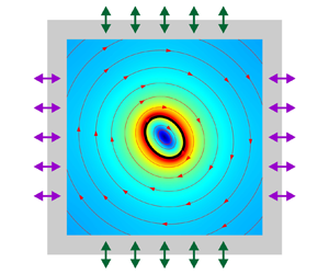
The time-averaged deformation dynamics of capsules driven by ultrasonic standing waves in a rectangular microfluidic cavity is investigated. Operating at the half-wavelength resonant frequency, the oscillations of two pairs of transducers connected to the cavity walls excite two orthogonal standing waves in the fluid cavity, as shown in figure 1(a). The pressure node is located at the centre of the cavity, and the pressure antinodes are located at the channel walls, as shown in figure 1(b). The capsule can be trapped at the centre of the cavity (i.e. at the pressure node) by the acoustic radiation force of the ultrasonic standing waves (Bernard et al. Reference Bernard, Doinikov, Marmottant, Rabaud, Poulain and Thibault2017). For the soft capsule trapped at the centre of the cavity, it not only experiences acoustic oscillations, but also exhibits complex time-averaged responses caused by the acoustic nonlinear effect.

Figure 1. (a) Schematic of a microfluidic cavity with a soft elastic capsule. (b) Illustration of 2-D ultrasonic standing waves (illustrated by dashed lines) generated by the oscillation of channel walls (illustrated by arrows).
The theoretical treatment of acoustical-induced capsule motion and deformation involves two completely separated time scale processes: the fast time scale for ultrasound propagation (usually in the microseconds range) and the slow time scale for the time-averaged response of the fluid and capsule (usually in the seconds range). To model this acoustic nonlinear phenomenon, the acoustic perturbation method in the context of generalized Lagrangian formulation (Nama, Huang & Costanzo Reference Nama, Huang and Costanzo2017) is employed in this work. Compared with the usual Eulerian formulation (Bruus Reference Bruus2012), the generalized Lagrangian formulation employs the perturbation expansion of fluid variables in the mean configuration. As shown in figure 2, the mean configuration is introduced as an intermediate configuration between the reference configuration and the current configuration. Here, the reference configuration  ${\mathrm{\mathcal{B}}_0}$ is the initial fluid configuration before acoustic excitation. In the acoustic field, the actual motion of the material particles is a combination of the mean motion ${\boldsymbol{u}_0}$ observed on the slow time scale and the acoustic oscillation $\boldsymbol{\xi }$ observed on the fast time scale. The mean motion of the material particles maps the reference configuration ${\mathrm{\mathcal{B}}_0}$ to the mean configuration $\mathrm{\mathcal{B}}$. The actual motion of the material particles maps the reference configuration ${\mathrm{\mathcal{B}}_0}$ to the current configuration ${\mathrm{\mathcal{B}}_t}$. Since the mean configuration $\mathrm{\mathcal{B}}$ is not disturbed by acoustic oscillations, it is convenient to formulate a theoretical framework in it, especially to accurately define the boundary conditions of the time-averaged dynamics. Therefore, the theoretical framework of this work is formulated in the mean configuration $\mathrm{\mathcal{B}}$.

Figure 2. Schematic of configurations used in this work, including the reference configuration  ${\mathrm{\mathcal{B}}_0}$ before acoustic excitation, mean configuration $\mathrm{\mathcal{B}}$ of particle time-averaged motion and current configuration ${\mathrm{\mathcal{B}}_t}$ of particle actual motion. Here, the actual motion of the material particles can be regarded as a combination of the mean motion ${\boldsymbol{u}_0}$ observed on the slow time scale and the acoustic oscillation $\boldsymbol{\xi }\rho \boldsymbol{v}$ observed on the fast time scale.
The hydrodynamics of the fluids is governed by the mass continuity equation and the momentum equation, which can be expressed in the mean configuration as
 \begin{gather}{\partial _t}\rho + \boldsymbol{F}_\xi ^{ - T}\boldsymbol{\cdot }\boldsymbol{\nabla }\rho \boldsymbol{\cdot }(\boldsymbol{v} - {\boldsymbol{v}_\xi }) + \rho \boldsymbol{F}_\xi ^{ - T}:\boldsymbol{\nabla v} = 0,\end{gather}
 \begin{gather}{J_\xi }\rho [{\partial _t}\boldsymbol{v} + \boldsymbol{\nabla v}\boldsymbol{\cdot }\boldsymbol{F}_\xi ^{ - 1}\boldsymbol{\cdot }(\boldsymbol{v} - {\boldsymbol{v}_\xi })] = \boldsymbol{\nabla }\boldsymbol{\cdot }\boldsymbol{P} + \boldsymbol{f},\end{gather}
where  $\rho$ is the fluid density, $\boldsymbol{v}$ is the fluid velocity, ${\boldsymbol{F}_\xi } = \boldsymbol{\nabla \xi }$ is the acoustic displacement gradient, ${J_\xi } = \det ({\boldsymbol{F}_\xi })$ is the Jacobian determinant of the acoustic displacement gradient, ${\boldsymbol{v}_\xi } = {\partial _t}\boldsymbol{\xi }$ is the time derivative of the acoustic displacement, $\boldsymbol{P}$ is the Piola–Kirchhoff stress of viscous compressible fluid and $\boldsymbol{f}$ represents the body force caused by the elastic tensions of the capsule membrane. The Piola–Kirchhoff stress $\boldsymbol{P}$ is related to the Cauchy stress $\boldsymbol{\sigma }$ through the relationship
 \begin{equation}\boldsymbol{P} = {J_\xi }\boldsymbol{\sigma }\boldsymbol{\cdot }\boldsymbol{F}_\xi ^{ - T},\end{equation}
where the superscript ‘ $- T$’ denotes the inverse transpose of the tensor. Equation (2.3) maps the Piola–Kirchhoff stress $\boldsymbol{P}$ defined as the force per unit area in the mean configuration $\mathrm{\mathcal{B}}$ to the Cauchy stress $\boldsymbol{\sigma }$ defined as the force per unit area in the current configuration ${\mathrm{\mathcal{B}}_t}$. Conversely, $\boldsymbol{\sigma } = J_\xi ^{ - 1}\boldsymbol{P}\boldsymbol{\cdot }\boldsymbol{F}_\xi ^T$ maps the Cauchy stress $\boldsymbol{\sigma }$ to the Piola–Kirchhoff stress $\boldsymbol{P}$. The Cauchy stress of the viscous compressible fluid is given by
 \begin{equation}\boldsymbol{\sigma } =- p\boldsymbol{I} + \mu ({\nabla _y}\boldsymbol{v} + {\nabla _y}{\boldsymbol{v}^T}) + \left( { - \tfrac{2}{3}\mu + {\mu_b}} \right)({\nabla _y} \boldsymbol{\cdot} \boldsymbol{v})\boldsymbol{I},\end{equation}
where  ${\nabla _y} = \boldsymbol{F}_\xi ^{ - 1}\boldsymbol{\cdot }\boldsymbol{\nabla }$ represents the gradient in the current configuration, $\mu $ and ${\mu _b}$ are the shear viscosity and bulk viscosity, respectively, and the fluid pressure p follows the relationship
 \begin{equation}p = c_0^2(\rho - {\rho _0}),\end{equation}
where  ${\rho _0}$ and ${c_0}$ are the density and sound speed of the stationary fluid, respectively. To obtain the governing equations for the two time scales, the acoustic perturbation method is employed, in which the fluid variables are expanded to the second order, $\{\,{\cdot}\,\} = {\{\,{\cdot}\, \} _0} + {\{\,{\cdot}\, \} _1} + {\{\,{\cdot}\, \} _2} + \cdots$, where the subscripts denote the respective orders. Correspondingly, (2.1) and (2.2) can be divided into a set of first-order equations governing the ultrasonic propagation on the fast time scale and second-order equations governing the time-averaged dynamics on the slow time scale.
2.1 Fast time scale wave propagation
According to the acoustic perturbation method, the first-order equations governing the acoustic wave propagation can be expressed in the frequency domain as
 \begin{gather}(\textrm{i}\omega ){p_1} + c_0^2{\rho _0}\nabla \boldsymbol{\cdot} {\textbf{v}_1} = 0\quad \textrm{and}\quad {\rho _0}(\textrm{i}\omega ){\boldsymbol{v}_1} = \boldsymbol{\nabla }\boldsymbol{\cdot }{\boldsymbol{P}_1},\end{gather}
 \begin{gather}{\boldsymbol{P}_1} =- {p_1}\boldsymbol{I} + \mu (\boldsymbol{\nabla }{\boldsymbol{v}_1} + \boldsymbol{\nabla v}_1^T) + ( - {\textstyle{2 \over 3}}\mu + {\mu _b})(\nabla \boldsymbol{\cdot }{\textbf{v}_1})\textbf{I}.\end{gather}
Here, all variables with subscript 1 correspond to first-order variables,  ${p_1}$ is the acoustic pressure, ${\boldsymbol{v}_1}$ is the acoustic particle velocity and $\omega = 2{\rm \pi} f$ is the angular frequency with f being the frequency. Since the acoustic impedance of the cell membrane is generally close to that of the cytoplasm, for ultrasound propagation, the cell membrane and the cytoplasm can be considered as a whole. As a model of the cell, the capsule membrane and the inner fluid are also considered as a whole. Therefore, the influence of the capsule membrane on acoustic propagation is neglected in (2.6).
Using the relationship  ${\boldsymbol{v}_1} = {\boldsymbol{v}_\xi } = (\textrm{i}\omega )\boldsymbol{\xi }$ with $\boldsymbol{\xi }$ being the acoustic particle displacement, the first-order equations (2.6) governing the acoustic wave propagation are given in terms of the acoustic particle displacement field $\boldsymbol{\xi }$ by
 \begin{equation}{\rho _0}{(\textrm{i}\omega )^2}\boldsymbol{\xi } - \boldsymbol{\nabla }\boldsymbol{\cdot }{\boldsymbol{P}_1}(\boldsymbol{\xi } )= \textbf{0},\end{equation}
with the first-order Piola–Kirchhoff stress
 \begin{equation}{\boldsymbol{P}_1}(\boldsymbol{\xi }) =- [c_0^2{\rho _0} + \textrm{i}\omega ( - {\textstyle{2 \over 3}}\mu + {\mu _b})](\boldsymbol{\nabla }\boldsymbol{\cdot }\boldsymbol{\xi })\textbf{I} + \textrm{i}\omega \mu (\boldsymbol{\nabla \xi } + \boldsymbol{\nabla }{\boldsymbol{\xi }^T}).\end{equation}
2.2 Slow time scale time-averaged dynamics
Now consider the time-averaged dynamics of the fluid–capsule system driven by the time-averaged acoustic force. According to the acoustic perturbation method, the time-averaged second-order equations governing the time-averaged dynamics can be expressed as
 \begin{equation}\boldsymbol{\nabla }\boldsymbol{\cdot }\langle {\boldsymbol{v}_2}\rangle = 0\quad \textrm{and}\quad \boldsymbol{\nabla }\boldsymbol{\cdot }\langle {\boldsymbol{P}_2}\rangle + \boldsymbol{f} = \textbf{0},\end{equation}
with the time-averaged second-order Piola–Kirchhoff stress
 \begin{align}
\langle {\boldsymbol{P}_2}\rangle & =- \langle \,{p_2}\rangle
\boldsymbol{I} + \mu (\boldsymbol{\nabla }\langle
{\boldsymbol{v}_2}\rangle + \boldsymbol{\nabla }{\langle
{\boldsymbol{v}_2}\rangle ^T})\notag\\ & \quad - \mu \langle
\boldsymbol{\nabla }{\boldsymbol{v}_1}\boldsymbol{\cdot
}\boldsymbol{\nabla \xi } + \boldsymbol{\nabla
}{\boldsymbol{\xi }^T}\boldsymbol{\cdot }\boldsymbol{\nabla
v}_1^T\rangle - ( - {\textstyle{2 \over 3}}\mu + {\mu
_b})\langle \boldsymbol{\nabla }{\boldsymbol{\xi
}^T}:\boldsymbol{\nabla }{\boldsymbol{v}_1}\rangle
\boldsymbol{I}\notag\\ &\quad + \langle
{\boldsymbol{P}_1}(\boldsymbol{\xi } )\boldsymbol{\cdot
}[(\boldsymbol{\nabla }\boldsymbol{\cdot }\boldsymbol{\xi
})\boldsymbol{I} - \boldsymbol{\nabla }{\boldsymbol{\xi
}^T}]\rangle .
\end{align}
\begin{align}
\langle {\boldsymbol{P}_2}\rangle & =- \langle \,{p_2}\rangle
\boldsymbol{I} + \mu (\boldsymbol{\nabla }\langle
{\boldsymbol{v}_2}\rangle + \boldsymbol{\nabla }{\langle
{\boldsymbol{v}_2}\rangle ^T})\notag\\ & \quad - \mu \langle
\boldsymbol{\nabla }{\boldsymbol{v}_1}\boldsymbol{\cdot
}\boldsymbol{\nabla \xi } + \boldsymbol{\nabla
}{\boldsymbol{\xi }^T}\boldsymbol{\cdot }\boldsymbol{\nabla
v}_1^T\rangle - ( - {\textstyle{2 \over 3}}\mu + {\mu
_b})\langle \boldsymbol{\nabla }{\boldsymbol{\xi
}^T}:\boldsymbol{\nabla }{\boldsymbol{v}_1}\rangle
\boldsymbol{I}\notag\\ &\quad + \langle
{\boldsymbol{P}_1}(\boldsymbol{\xi } )\boldsymbol{\cdot
}[(\boldsymbol{\nabla }\boldsymbol{\cdot }\boldsymbol{\xi
})\boldsymbol{I} - \boldsymbol{\nabla }{\boldsymbol{\xi
}^T}]\rangle .
\end{align} Here, all variables with subscript 2 correspond to second-order variables,  $\langle {\boldsymbol{v}_2}\rangle $ is the second-order fluid velocity and $\langle \,{p_2}\rangle $ is the second-order fluid pressure determined by the incompressible constraint given in the first of (2.10). The first line in (2.11) represents the stress of incompressible fluid, while the second line of (2.11) consists of the products of two acoustic quantities, representing the driving force for the time-averaged response of the capsule and surrounding fluid. The flow $\langle {\boldsymbol{v}_2}\rangle $ includes two components, the acoustic streaming $\langle \boldsymbol{v}_2^a\rangle $ generated by the driving term in (2.11) and the Stokes flow $\langle \boldsymbol{v}_2^s\rangle$ driven by the motion and deformation of the capsule. Fluid viscosity plays an important role in the driving term, so acoustic streaming can be explained as a result of acoustic dissipation.
The membrane of the 2-D capsule is geometrically regarded as a closed 1-D curve marked by the position  ${\boldsymbol{x}_c}$ in the mean configuration. The unit tangent vector $\boldsymbol{t}$ of the membrane points in the direction of increasing arc length, and the unit normal vector $\boldsymbol{n}$ points to the outer fluid. For later use, the curve gradient and curve divergence operators for vector fields are introduced as (Steinmann Reference Steinmann2008)
 \begin{equation}{\nabla _c}\{\,{\cdot}\, \} = {\partial _l}\{\,{\cdot}\, \} \otimes \boldsymbol{t}\quad \textrm{and}\quad {\nabla _c}\boldsymbol{\cdot }\{\,{\cdot}\, \} = {\partial _l}\{\,{\cdot}\, \} \boldsymbol{\cdot }\boldsymbol{t}.\end{equation}
 Here, the curve gradient and curve divergence operators on the left are expressed in vector form and independent of the coordinate system (i.e. local curve coordinates and global Cartesian coordinates). Based on the thin-shell formulation (Pozrikidis Reference Pozrikidis2001), the equilibrium equation for the capsule membrane under the action of the traction  $\boldsymbol{f}$ (in $\textrm{N}\;{\textrm{m}^{ - 2}}$) can be derived as
 \begin{equation}\boldsymbol{f} = {\nabla _c}\boldsymbol{\cdot }(\tau \boldsymbol{t} \otimes \boldsymbol{t} + \boldsymbol{n} \otimes {\nabla _c}m),\end{equation}
where  $\tau $ (in $\textrm{N}\;{\textrm{m}^{ - \textrm{1}}}$) is the in-plane tension and m (in $\textrm{N}\;\textrm{m}$) is the bending moment.
The in-plane tension and bending moment are given by constitutive laws of the capsule membrane material. To this end, the neo-Hookean model is employed to obtain the in-plane tension, where the neo-Hookean model allows for area dilatation. In fact, some types of cells have extensible membranes, such as keratocytes (Shao, Rappel & Levine Reference Shao, Rappel and Levine2010) and fibroblasts (Raucher & Sheetz Reference Raucher and Sheetz1999), and the membrane area of these cells can be altered by the flattening of small-scale wrinkles. There are also types of cells whose membranes are considered to be (close to) inextensible, such as red blood cells (Cordasco & Bagchi Reference Cordasco and Bagchi2014). The capsules studied here are more representative of those cells that are extensible, so the application of the neo-Hookean model is accurate. In particular, it has been shown that the neo-Hookean model is effective in capturing the characteristics of cells regardless of whether the cell membranes allow for area dilatation (Bagchi Reference Bagchi2007; Jayathilake et al. Reference Jayathilake, Liu, Tan and Khoo2011; Luo et al. Reference Luo, Wang, He, Lu, Xu and Bai2013). The in-plane tension of the capsule membrane line segments is calculated as (Bagchi, Johnson & Popel Reference Bagchi, Johnson and Popel2005)
 \begin{equation}\tau = {E_s}(J_c^{{3 / 2}} - J_c^{ - {3 / 2}}),\end{equation}
where  ${E_s}$ is the membrane elastic modulus and ${J_c}$ is the stretch ratio of the membrane, which is calculated from the evolution equation (Ii et al. Reference Ii, Shimizu, Sugiyama and Takagi2018):
 \begin{equation}{\partial _t}{J_c} + \langle {\boldsymbol{v}_2}\rangle \boldsymbol{\cdot }{\nabla _c}{J_c} = ({\nabla _c}\boldsymbol{\cdot }\langle {\boldsymbol{v}_2}\rangle ){J_c}.\end{equation}
In (15), the continuity boundary condition of the membrane velocity and fluid velocity, i.e.  ${\boldsymbol{v}_c} = \textrm{d}{\boldsymbol{x}_c}/\textrm{d}t = \langle {\boldsymbol{v}_2}\rangle $, is used. Additionally, the bending moment is determined by the Helfrich bending energy as (Helfrich Reference Helfrich1973)
 \begin{equation}m = {E_b}(h - {h_0}),\end{equation}
where  ${E_b}$ is the membrane bending modulus, and h and ${h_0}$ are the curvature of the membrane in the mean and reference configuration, respectively. The curvature ${h_0}$ is not the spontaneous curvature associated with lipid membranes. The curvature h is calculated from the curvature vector $\boldsymbol{h} \equiv h\boldsymbol{n}$, which obeys (Elliott & Stinner Reference Elliott and Stinner2010)
 \begin{equation}\boldsymbol{h} =- {\nabla _c}\boldsymbol{\cdot }{\boldsymbol{i}_c}.\end{equation}
Here,  ${\boldsymbol{i}_c} = \boldsymbol{I} - \boldsymbol{n} \otimes \boldsymbol{n} = \boldsymbol{t} \otimes \boldsymbol{t}$ is the curve unit tensor. The curvature ${h_0}$ is a variable in the reference configuration. It can be updated as a state variable in the mean configuration according to the advection equation, defined as
 \begin{equation}{\partial _t}{h_0} + \langle {\boldsymbol{v}_2}\rangle \boldsymbol{\cdot }{\nabla _c}{h_0} = 0.\end{equation}
3. Finite element model
As shown in figure 3(a), the calculation domain is the square of the length  $L = 100\;{\rm \mu} \mathrm{m}$. The whole calculation domain is occupied by the water-based biological solution with a capsule immersed in it. All relevant material parameters are listed in table 1. The model system has a half-wavelength resonance given by the frequency $f = c_0^{out}/(2L) = 7.475\;\textrm{MHz}$. To excite this resonance, the external acoustic excitations have a harmonic time dependence of frequency $f = 7.475\;\textrm{MHz}$. In what follows, to facilitate the numerical implementation based on the finite element method, the strong form of the governing equations introduced in the above section is transformed into a weak form.

Figure 3. (a) Finite element model. The whole fluid domain is represented by  $\mathrm{\mathcal{B}}$ and the capsule membrane is denoted by $\mathrm{\mathcal{C}}$. The domain defined by the dashed line representing the fluid domain does not include the viscous boundary layer around the walls with the viscous boundary layer thickness ${\delta _v} = \sqrt {2{\mu ^{out}}/(\rho _0^{out}\omega )} \approx 0.20\;{\rm \mu} \mathrm{m}$. (b) Typical mesh and enlargement of the capsule area used in the simulation.
Table 1. Model parameters of capsules. These parameters are chosen with reference to the parameters of red blood cells (Muller et al. Reference Muller, Barnkob, Jensen and Bruus2012; Mishra et al. Reference Mishra, Hill and Glynne-Jones2014).

By multiplying (2.8) with the test function  $\delta \boldsymbol{\xi }$ of the acoustic displacement $\boldsymbol{\xi }$, integrating over the fluid domain $\mathrm{\mathcal{B}}$ and applying the divergence theorem, the weak form of the acoustic wave equation is obtained as
 \begin{equation}\int_\mathrm{\mathcal{B}} {[{\rho _0}{{(\textrm{i}\omega )}^2}\boldsymbol{\xi }\boldsymbol{\cdot }\delta \boldsymbol{\xi } + {\boldsymbol{P}_1}:\nabla \boldsymbol{\xi }]\,\textrm{d}a} = 0.\end{equation}
The two acoustic excitations on the oscillating walls are expressed in terms of acoustic particle displacement as
 \begin{gather}\boldsymbol{\xi } = {u_0}\,{\textrm{e}^{\textrm{i}\omega t}}{\boldsymbol{e}_x}\quad \textrm{for}\;\boldsymbol{x} \in {\varGamma ^{left}} \cup {\varGamma ^{right}},\end{gather}
 \begin{gather}\boldsymbol{\xi } = {u_0}\,{\textrm{e}^{\textrm{i}\omega t + \textrm{i}\varphi }}{\boldsymbol{e}_y}\quad \textrm{for}\;\boldsymbol{x} \in {\varGamma ^{top}} \cup {\varGamma ^{bottom}},\end{gather}
where  ${u_0}$ is the input particle displacement amplitude, $\varphi $ is the phase difference between two excitation signals, and ${\varGamma ^{left}}$, ${\varGamma ^{right}}$, ${\varGamma ^{top}}$ and ${\varGamma ^{bottom}}$ denote the left, right, top and bottom walls, respectively.
Similarly, by multiplying (2.10) with the test function pairs  $(\delta \langle \,{p_2}\rangle ,\delta \langle {\boldsymbol{v}_2}\rangle )$ of the second-order pressure and second-order velocity $(\langle \,{p_2}\rangle ,\langle {\boldsymbol{v}_2}\rangle )$, integrating over the fluid domain $\mathrm{\mathcal{B}^{\prime}}$ and applying the divergence theorem, the weak form of the fluid dynamic equation can be obtained as
 \begin{gather}\int_{\mathrm{\mathcal{B}^{\prime}}} {(\boldsymbol{\nabla }\boldsymbol{\cdot }\langle {\boldsymbol{v}_2}\rangle )\boldsymbol{\cdot}\delta \langle \,{p_2}\rangle \,\textrm{d}a} = 0,\end{gather}
 \begin{gather}- \int_{\mathrm{\mathcal{B}^{\prime}}} {\langle {\boldsymbol{P}_2}\rangle :\boldsymbol{\nabla }\delta \langle {\boldsymbol{v}_2}\rangle \,\textrm{d}a} + \int_\mathrm{\mathcal{C}} {\boldsymbol{f}\boldsymbol{\cdot }\delta \langle {\boldsymbol{v}_2}\rangle \,\textrm{d}l} = 0,\end{gather}
where  $\mathrm{\mathcal{B}^{\prime}}$ represents the fluid domain excluding the acoustic viscous boundary layer near the channel walls (the domain defined by the dashed line in figure 3a). The integrating domain is chosen to exclude acoustic streaming generated by acoustic dissipation in the viscous boundary layer near the channel wall. The effect of this boundary-drive acoustic streaming on capsule dynamics is negligible because the acoustic streaming becomes zero in the central part of the fluid domain (where the capsule is captured). Furthermore, using (2.13) and applying the curve divergence theorem, (3.5) becomes
 \begin{equation}- \int_{\mathrm{\mathcal{B}^{\prime}}} {\langle {\boldsymbol{P}_2}\rangle :\boldsymbol{\nabla }\delta \langle {\boldsymbol{v}_2}\rangle \,\textrm{d}a} - \int_\mathrm{\mathcal{C}} {(\tau \boldsymbol{t} \otimes \boldsymbol{t} + \boldsymbol{n} \otimes {\nabla _c}m):\boldsymbol{\nabla }\delta \langle {\boldsymbol{v}_2}\rangle \,\textrm{d}l} = 0.\end{equation}
In the second term of (3.6), the tension  $\tau $ is a function of the stretch ratio ${J_c}$. According to (2.15), the stretch ratio ${J_c}$ is solved from the following weak form equation:
 \begin{equation}\int_\mathrm{\mathcal{C}} {[{\partial _t}{J_c} + \langle {\boldsymbol{v}_2}\rangle \boldsymbol{\cdot }{\nabla _c}{J_c} - ({\nabla _c}\boldsymbol{\cdot }\langle {\boldsymbol{v}_2}\rangle ){J_c}] \boldsymbol{\cdot} \delta {J_c}\,\textrm{d}l} = 0,\end{equation}
where  $\delta {J_c}$ is the corresponding test functions of ${J_c}$. The moment m is a function of the curvature h and ${h_0}$. According to (2.17) and (2.18), the curvature h and ${h_0}$ are solved from the following weak form equations:
 \begin{gather}\int_\mathrm{\mathcal{C}} {(\boldsymbol{h}\boldsymbol{\cdot }\delta \boldsymbol{h} - {\boldsymbol{i}_c}\textrm{:}{\nabla _c}\delta \boldsymbol{h})\,\textrm{d}l} = 0,\end{gather}
 \begin{gather}\int_\mathrm{\mathcal{C}} {({\partial _t}{h_0} + \langle {\boldsymbol{v}_2}\rangle \boldsymbol{\cdot }{\nabla _c}{h_0})\boldsymbol{\cdot }\delta {h_0}\,\textrm{d}l} = 0,\end{gather}
where  $\delta \boldsymbol{h}$ and $\delta {h_0}$ are the corresponding test functions of $\boldsymbol{h}$ and $\delta {h_0}$, respectively. Furthermore, for the time-averaged dynamic problem, the no-slip boundary condition is imposed on the boundary of the computational domain $\mathrm{\mathcal{B}^{\prime}}$ as
 \begin{equation}\langle {\boldsymbol{v}_2}\rangle = \textbf{0}\quad \textrm{for}\;\boldsymbol{x} \in \partial \mathrm{\mathcal{B}^{\prime}}.\end{equation}
To fix the numerical solution of the incompressible time-averaged flow, a pressure point constraint is imposed at the point  $\mathrm{\mathcal{P}}$ in figure 3(a) as
 \begin{equation}\langle \,{p_2}\rangle = 0\quad \textrm{at}\;\mathrm{\mathcal{P}}.\end{equation}
 The weak form governing equations are solved in the commercial finite element software COMSOL Multiphysics. Specifically, the acoustic wave equation (3.1) along with the boundary conditions (3.2) and (3.3) are implemented in the ‘weak form partial differential equation (PDE)’ interface, the time-averaged dynamic equations (3.4) and (3.6) are implemented by modifying the ‘laminar two-phase flow, moving mesh’ interface, and the additional equations (3.7)–(3.9) used for calculating  ${J_c}$, $h$ and ${h_0}$ are implemented in the ‘weak form boundary PDE’ interface. It is worth noting that in the ‘laminar two-phase flow, moving mesh’ interface, the moving mesh technique is used to track the interface of the membrane. To obtain the smooth solutions, $\boldsymbol{\xi }$, ${J_c}$, $h$ and ${h_0}$ are approximated with the third-order Lagrange elements, and $(\langle {\boldsymbol{v}_2}\rangle ,\langle \,{p_2}\rangle )$ are approximated with third-order Lagrangian elements for $\langle {\boldsymbol{v}_2}\rangle $ and second-order composite Lagrangian elements for $\langle \,{p_2}\rangle$ to meet the stability requirements of incompressible flow. All governing equations are solved simultaneously by the time-dependent solver, and the time step in the range of ${10^{ - 3}} \sim {10^{ - 4}}\;\textrm{s}$ depends on the displacement excitation amplitude. The typical mesh used in the simulations is shown in figure 3(b).
4. Results and discussion
4.1 Model validation
The developed numerical model can simulate the time-averaged deformation dynamics of capsules driven by ultrasonic standing waves. To validate the present numerical model, considering zero acoustic input, the present numerical model is degraded to calculate the transient deformation of a capsule in shear flow and compared with previous results (Breyiannis & Pozrikidis Reference Breyiannis and Pozrikidis2000). As shown in figure 4, the initially circular capsule is considered in a simple shear flow with constant shear rate k. The capsule membrane obeys Hooke's law, which assumes a linear constitutive relation as  $\tau = {E_s}({J_c} - 1)$. The fluids inside and outside the capsule have the same shear viscosity $\mu $, and their motion is described by the Stokes flow equation ignoring the inertial effect. The dynamics of the capsule is controlled by the capillary number $Ca = \mu k{a_0}/{E_s}$, which measures the ratio of viscous force to elastic force.

Figure 4. Schematic of an initially circular capsule in shear flow.
The tank-treading motion of the capsule in the shear flow is captured by the present finite element model. The capsule deforms from the initially circular shape to an elliptical shape and remains in a stable state, while the capsule membrane still rotates around the inside fluid driven by the shear force of the surrounding fluid. The deformation of the capsule is characterized by the Taylor shape parameter  $D = ({a_1} - {a_2})/({a_1} + {a_2})$, with ${a_1}$ and ${a_2}$ being the major and minor semi-axes of the deformed elliptical shape, respectively, and the inclination angle $\theta $ relative to the positive $x$-axis (see figure 4). The time evolution of D and $\theta $ for different $Ca$ are presented in figure 5(a,b), respectively. The present results are shown to match the previous results obtained by boundary integral simulations (Breyiannis & Pozrikidis Reference Breyiannis and Pozrikidis2000).

Figure 5. Time-evolution of capsules in simple shear flow for different capillary numbers  $Ca$: (a) deformation index D; (b) inclination angle $\theta $. Note that in figure 2 of the previous paper (Breyiannis & Pozrikidis Reference Breyiannis and Pozrikidis2000), the results for $Ca = 0.05$ are incorrectly labelled as $Ca = 0.04$ (Mendez, Gibaud & Nicoud Reference Mendez, Gibaud and Nicoud2014).
4.2 Circular capsules in 2-D standing waves
This subsection studies the dynamics of the initially circular capsule in 2-D standing waves generated by the oscillation of the top/bottom wall pair and left/right wall pair at different phase differences  $\varphi $. In the present work, the initial shape of the capsule is its stress-free shape. The displacement excitation amplitude of the ultrasonic excitation is fixed at ${u_0} = {10^{ - 11}}\;\textrm{m}$, and the induced acoustic pressure amplitude in the microfluidic cavity is approximately $0.5\;\textrm{MPa}$. As will be discussed in figures 6–8, for the initially circular capsule, there are three dynamic states: pure elongation deformation, pure rotation motion and tank-treading motion. The pure elongation deformation occurs when the phase difference is $\varphi = 0$. The pure rotation motion occurs when the phase difference is $\varphi = {\rm \pi}/2$. The tank-treading motion occurs when the phase difference is between $\varphi = 0$ and $\varphi = {\rm \pi}/2$.

Figure 6. (a) RMS acoustic pressure around the capsule in the initial state. (b) Flow pattern around the capsule in the steady state. The red line indicates the capsule membrane, and the phase difference is  $\varphi = 0$. In this case, the capsule is elongated along the along the acoustic pressure nodal line $y =- x$.
For the phase difference  $\varphi = 0$, figure 6(a) plots the root-mean-square (RMS) acoustic pressure around the capsule in the initial state with red circles representing the capsule membrane. It can be observed from figure 6(a) that the acoustic pressure has a static nodal line (blue) along $y =- x$, while the amplitude is oscillating. This acoustic pressure pattern is similar to that of the 1-D standing wave with the nodal line along $y =- x$. Therefore, the capsule dynamics in a 2-D standing wave with phase difference $\varphi = 0$ is similar to that in 1-D standing waves. Figure 6(b) shows the flow pattern of the acoustic streaming $\langle \boldsymbol{v}_2^a\rangle $ around the stretched capsule in the steady state, whereas the Stokes flow $\langle \boldsymbol{v}_2^s\rangle $ driven by the membrane motion is zero due to the zero velocity of the capsule membrane in the steady state. Outside the capsule, the outer acoustic streaming is expelled in the direction perpendicular to the acoustic pressure nodal line, while the inner acoustic streaming is characterized by the vortex structure rotating in the opposite direction. Inside the capsule, the acoustic streaming consists of four vortices. As shown in figure 6(a,b), in the 2-D ultrasonic standing wave field, the capsule is stretched along the acoustic pressure nodal line and finally reaches a steady state of pure elongation deformation. Here, the time-averaged stress generated by 2-D ultrasonic standing waves has normal and tangential components. The normal stress deforms the capsule and tangential stress rotates the capsule. The clockwise and counterclockwise components of the tangential stress cancel each other, no rotation motion is produced, and only the stable elongation deformation caused by the normal stress is present (see figure 17 in § 4.4). Therefore, when the phase difference is $\varphi = 0$, the capsule undergoes pure elongation deformation.
For the phase differences  $\varphi = {\rm \pi}/2$, figure 7(a) plots the RMS acoustic pressure around the capsule in the initial state. The acoustic field around the capsule is shown to be approximately a vortex beam with zero amplitude at the core. Figure 7(b) shows the flow pattern around the capsule in the steady state. For an initially circular capsule, this rotationally symmetric acoustic field does not cause any obvious deformation of the capsule. However, the capsule is observed to rotate in the clockwise direction. Around the capsule membrane, the total flow consists of the rotating acoustic streaming $\langle \boldsymbol{v}_2^a\rangle $ generated by acoustic dissipation and the rotating Stokes flow $\langle \boldsymbol{v}_2^s\rangle $ generated by capsule rotation. Thus, the terminal rotation speed is determined by the moment balance generated by the acoustic streaming and the moment generated by the Stokes flow. In particular, the moment generated by the acoustic streaming induces the capsule rotation, while the moment generated by the Stokes flow acts as a hindrance. As the effect of inertia is negligible, the capsule immediately reaches a steady state of pure rotation motion. As mentioned above, the time-averaged stress generated by 2-D ultrasonic standing waves has normal and tangential components. The normal stress deforms the capsule and tangential stress rotates the capsule. Here, the normal stress is zero and no elongation deformation is produced, and only the stable rotation motion caused by the clockwise tangential stress is present (see figure 17 in § 4.4). Therefore, when the phase difference is $\varphi = {\rm \pi}/2$, the capsule undergoes pure rotation motion.

Figure 7. (a) RMS acoustic pressure around the capsule in the initial state. (b) Flow pattern around the capsule in the steady state. The red line indicates the capsule membrane, and the phase difference is  $\varphi = {\rm \pi}/2$. In this case, the capsule rotates clockwise with an angular frequency of 0.45 rps (revolution per second).
For the phase difference between  $\varphi = 0$ and $\varphi = {\rm \pi}/2$, figure 8(a,b) plot the time evolution of the deformation index D and inclination angle $\theta $ of the capsule at different phase differences $\varphi = 15{\rm \pi}/64$, $25{\rm \pi}/64$ and $30{\rm \pi}/64$. The capsule is shown to take approximately $0.2\;\textrm{s}$ to reach a steady state. Figure 8(c) further plots the flow pattern around the capsule membrane in the steady state. The results show that the capsule at the steady state exhibits a stable tank-treading motion, just like suspended in a shear flow. It is known that the shear flow can be divided into elongation and rotation components, so the capsule performs the tank-treading motion. As discussed in figures 6 and 7, the capsule undergoes pure elongation deformation for the phase difference $\varphi = 0$ and pure rotation motion for the phase difference $\varphi = {\rm \pi}/2$. Here, similar to shear flow, the 2-D standing wave with the phase difference between $0$ and ${\rm \pi}/2$ also produces a combined effect of elongation and rotation on the capsule, the normal stress deforms the whole capsule and the tangential stress rotates the capsule membrane. The capsule deformation and membrane rotation as a whole form the tank-treading motion. Since the initially circular capsule has no energy barrier (see Appendix A for details) for the tank-treading motion, the initially circular capsule performs the stable tank-treading motion at a fixed inclination angle. Therefore, when the phase difference is between $\varphi = 0$ and $\varphi = {\rm \pi}/2$, the capsule undergoes tank-treading motion.

Figure 8. (a) Time evolution of deformation index and inclination angle at different phase differences  $\varphi = 15{\rm \pi}/64$, $25{\rm \pi}/64$ and $30{\rm \pi}/64$; (b) the shape of the capsule (indicated by the red line) and the flow pattern around the capsule in the steady state.
Moreover, it can be seen from figure 8(a,c) that increasing the phase difference weakens the elongation effect, so that the deformation of the capsule decreases with increasing the phase difference, while increasing the phase difference strengthens the rotation effect, so that the tank-treading speed of the capsule membrane increases with increasing the phase difference (indicated by the increased mean flow velocity). Figure 8(b) shows that the inclination angle decreases as the phase difference increases. For the deformed capsule, the 2-D standing wave generates two moments acting on it: one moment aligns the long axis of the deformed capsule along the inclination angle  $3{\rm \pi}/4$, related to the elongation effect, and the other moment rotates the capsule clockwise, related to the rotation effect. As the phase difference increases, the former moment decreases, while the latter moment increases. Thus, as the phase difference increases, the acoustic-induced moment tends to rotate the capsule clockwise away from the inclination angle $3{\rm \pi}/4$, and the inclination angle is observed to decrease.
Here, the effect of membrane elasticity on the capsule dynamics is examined. Figure 9 plots the dynamic parameters, including steady-state deformation index D, inclination angle  $\theta $ and tank-treading angular velocity ${\omega ^{tt}}$, as a function of the phase difference $\varphi $ for different shear moduli ${E_s}$. As discussed in figures 6 and 7, as the phase difference increases from $0$ to ${\rm \pi}/2$, the effect of the 2-D standing waves on the capsule changes from pure elongation to pure rotation. Therefore, the deformation index D and inclination angle $\theta $ decrease, while the tank-treading angular velocity ${\omega ^{tt}}$ increases. This observation is essentially the same as that observed in figures 6–8. For a fixed phase difference, with the increase of the shear modulus, the deformation index D decreases, while the inclination angle $\theta $ and the tank-treading angular velocity ${\omega ^{tt}}$ increase. Figure 10 plots the dynamic parameters, including steady-state deformation index D, inclination angle $\theta $ and tank-treading angular velocity ${\omega ^{tt}}$, as a function of the phase difference $\varphi $ for different bending moduli ${E_b}$. As shown in figure 10, as the bending modulus ${E_b}$ decreases, the steady-state deformation index D decreases, while the inclination angle $\theta $ and the tank-treading angular velocity ${\omega ^{tt}}$ increase. These trends are generally the same as those observed when increasing the shear modulus. Regarding the effect on the capsule dynamics, the shear modulus and bending modulus of the membrane are similar in that they both limit the deformation of the capsule. It can also be seen that the deformation index and inclination angle are more sensitive to the shear modulus when the phase difference is small, while the deformation index and inclination angle are more sensitive to the bending modulus when the phase difference is large.

Figure 9. Effects of shear modulus on capsule dynamics: (a) deformation index; (b) inclination angle; (c) tank-treading angular velocity.

Figure 10. Effects of bending modulus on capsule dynamics: (a) deformation index; (b) inclination angle; (c) tank-treading angular velocity.
The trend of the dynamic parameters of the tank-treading capsule in relation to the elastic modulus of the membrane, including the shear modulus and bending modulus, is analysed. First, it is most obvious that increasing the shear modulus and bending modulus constrains the deformation of the capsule, which leads to smaller deformations, as shown in figures 9(a) and 10(a). Then, the trend of the tank-treading angular velocity can be explained based on the results of capsule deformation. With a larger elastic modulus, the smaller deformation reduces the velocity gradient around the capsule and the capsule membrane is more likely to circulate around the capsule contour. Therefore, as shown in figures 9(c) and 10(c), the tank-treading angular velocity increases as the elastic moduli increase. Finally, figures 9(b) and 10(b) show that the steady-state inclination angle increases with the increase of the elastic modulus. The steady-state inclination angle is determined by the balance between the acoustic-induced moment and the Stokes flow-induced moment. Here, the tank-treading membrane drives a clockwise rotating Stokes flow, which in turn exerts a reaction moment that tends to rotate the capsule counterclockwise. This Stokes flow induced reaction moment increases with the increase of the tank-treading angular velocity. With the increase of the shear modulus and bending modulus, the counterclockwise deflection of the inclination angle (i.e. the increase of the inclination angle) is related to the increase of the tank-treading angular velocity, as shown in figures 9(b) and 10(b). That is, with the increase of shear modulus and bending modulus, the capsule deformation decreases, the clockwise tank-treading angular velocity increases and the counterclockwise Stokes flow moment increases, leading to the counterclockwise deflection of the capsule inclination angle, i.e. the inclination angle increases in figures 9(b) and 10(b). It is noticed that this trend is not significant at small phase differences. This is because at small phase differences, the clockwise and counterclockwise tangential stresses largely cancel each other out (see figure 17 in § 4.4), resulting in a weak rotation effect and small tank-treading angular velocity for all considered shear and bending moduli, as shown in figures 9(c) and 10(c). Accordingly, the small tank-treading motion induces a small Stokes flow, and also the small Stokes flow-induced moment has a small effect on the steady-state inclination angle, which limits the influence of membrane elasticity on the steady-state inclination angle.
Figure 11 shows the effect of internal fluid viscosity on the initially circular capsule dynamics, where the dynamic parameters of the tank-treading motion including the steady-state deformation index D, inclination angle  $\theta $ and tank-treading angular velocity ${\omega ^{tt}}$ are plotted as a function of the phase difference $\varphi $ for different internal fluid viscosities ${\mu ^{in}}$. As shown in figure 11(a), the internal fluid viscosity has little effect on the deformation of the capsule. The internal fluid viscosity affects the deformation of the capsule through the viscous shear stress generated by the velocity gradient. In the steady state, the internal fluid velocity is small (see figures 6b and 8c) and the viscous shear stress generated by the internal fluid viscosity is also small. Therefore, the internal fluid viscosity has little effect on the steady-state deformation of the capsule. Only at large phase differences, the internal fluid velocity becomes large [see figure 8c] and the internal fluid viscosity generates large viscous shear stress, which slightly affects the capsule deformation. As shown in figure 11(b), when the internal fluid viscosity increases, the inclination angle decreases. The high internal fluid viscosity hinders the clockwise motion of the capsule membrane driven by acoustic streaming. That is, the high internal fluid viscosity makes the capsule membrane and the internal fluid more like a whole, and the acoustic streaming drives the capsule membrane and internal fluid as a whole to deflect clockwise (corresponding the decrease of the inclination angle). Therefore, the increase of the internal fluid viscosity leads to the decrease of the inclination angle.

Figure 11. Effect of internal fluid viscosity on capsule dynamics: (a) deformation index; (b) inclination angle; (c) tank-treading angular velocity.
As shown in figure 11(c), when the phase difference  $\varphi $ is in the wide range of $[0,\textrm{0}\mathrm{.45}{\rm \pi} ]$, the tank-treading angular velocity decreases as the internal fluid viscosity increases, while the trend is reversed when the phase angle $\varphi $ is close to $0.5{\rm \pi}$. A greater internal fluid viscosity results in a greater resistance of the internal Stokes flow to the membrane tank-treading motion. Additionally, a greater internal fluid viscosity results in a greater acoustic energy dissipation of the whole acoustic field, a greater velocity of the external acoustic streaming generated by the acoustic energy dissipation and a greater driving force for the membrane tank-treading motion. Considering that it is the change of internal fluid viscosity, the effect of internal viscosity on internal Stokes flow is greater than the effect on external acoustic streaming in the above two effects. Therefore, in the wide phase difference range of $[0,\textrm{0}\mathrm{.45}{\rm \pi} ]$, the internal Stokes flow plays a dominant role, and a greater internal fluid viscosity results in a greater resistance of the internal Stokes flow to the membrane tank-treading motion and a slower membrane tank-treading angular velocity. However, when the phase difference $\varphi $ is $0.5{\rm \pi}$ (or close to $0.5{\rm \pi}$), the capsule does not deform and maintains its initially circular shape, the capsule membrane and the internal fluid rotate together as a whole (Keller & Skalak Reference Keller and Skalak1982), so that the internal Stokes flow does not resist the motion of the capsule membrane, and the external acoustic streaming plays a dominant role in this case. Therefore, when the phase difference $\varphi $ is $0.5{\rm \pi}$ (or close to $0.5{\rm \pi}$), a greater internal fluid viscosity results in a greater driving force for the membrane tank-treading motion and a faster membrane tank-treading angular velocity.
4.3 Elliptical capsules in 2-D standing waves
Initial non-spherical biological particles are common in the biological system, such as biconcave erythrocytes. In this subsection, the numerical model is used to study the elliptical capsule to qualitatively understand the dynamics of real non-spherical biological particles. For a capsule with an initial elliptical shape whose area is set equal to a circle of radius  ${a_0}$, the initial conditions are provided by the initial aspect ratio ${\alpha _0} = {a_2}/{a_1}$ and the initial orientation ${\theta _0}$, where ${a_1}$ and ${a_2}$ are the major and minor semi-axes of the elliptical shape. The initial orientation is fixed at ${\theta _0} = {\rm \pi}/2$ in the following simulations.
As shown in figure 12(a), the phase diagram for different dynamical states is plotted as a function of the displacement excitation amplitude and phase difference at the initial aspect ratio of  ${\alpha _0} = 0.8$. At the displacement excitation amplitude of ${u_0} = 0.32 \times {10^{ - 11}}\;\textrm{m}$, as the phase difference increases, the dynamic state of the capsule changes from the stable orientation (green circle) to tumbling motion (red square). At the displacement excitation amplitude of ${u_0} = 1 \times {10^{ - 11}}\;\textrm{m}$, as the phase difference increases, the dynamic state of the capsule changes from the stable orientation (green circle) to swinging motion (blue rhombus), and then to tumbling motion (red square). For the initially non-circular capsule, there are three dynamical states including stable orientation, tumbling motion and swinging motion, according to the dynamical characteristics of the capsule inclination angle and the membrane material points. In the stable orientation, the capsule inclination angle eventually reaches a steady state, in which the inclination angle remains unchanged over time. This is illustrated by the time evolution of the capsule inclination angle as shown by the green dash curve in figure 12(b). In addition, the blue and pink points in figure 12(c) show two material points of the capsule membrane. The material points are shown to remain stationary in the steady state (i.e. stable orientation). In the tumbling motion, the capsule inclination angle undergoes a complete $2{\rm \pi}$ rotation. The rapid decrease of the capsule inclination angle with time shown by the red solid curve in figure 12(b) corresponds to the capsule tumbling motion. The motion of the membrane material points in figure 12(e) is caused by the rigid-body-like rotation of the capsule, which does not circulate around its contour. In the swinging motion, the capsule membrane performs tank-treading motion and the capsule inclination angle oscillates with time, but never makes a $2{\rm \pi}$ rotation. This is illustrated by the fluctuation of the capsule inclination angle with time as shown by the blue dash–dotted curve in figure 12(b). The capsule membrane also circulates clockwise around its contour as shown by the motion of the material points in figure 12(d).

Figure 12. (a) Phase diagram of different dynamical states as a function of displacement excitation amplitude and phase difference. (b) Typical time evolution curves of deformation index and inclination angle for stable orientation, swinging and tumbling. (c–e) Shapes and flow profiles of stable orientation, swinging and tumbling represented by hollow circles, hollow diamonds and hollow squares in panel (b), respectively. The blue and pink particles are attached to the capsule membrane, and the red dashed lines indicate the orientation of the major axis. Supplementary movies are available at https://doi.org/10.1017/jfm.2023.277.
In figure 12, as mentioned above, for the initially non-circular capsule, there are three dynamic states: stable orientation, tumbling motion and swinging motion. The time-averaged stress generated by 2-D ultrasonic standing waves has normal and tangential components. The normal stress deforms the capsule and tangential stress rotates the capsule.
(1) Stable orientation: When the phase difference is relatively small, the clockwise and counterclockwise components of the tangential stress cancel each other, no rotation motion is produced and only the stable elongation deformation caused by the normal stress is present. The initially circular capsule is stable elongation deformation, and the initially non-circular capsule is also stable elongation deformation, but called stable orientation, since its long axis has a stable inclination angle.
(2) Tumbling motion: When the phase difference is relatively large, the normal stress causes elongation deformation and the initially non-circular capsule deforms into another ellipse with greater curvature. If the work provided by the acoustic streaming is insufficient to overcome the energy barrier of the tank-treading motion (see Appendix A for details), the membrane elements do not start cycling around the elliptical capsule contour, and the moment formed by the clockwise tangential stress causes the overall tumbling motion of the capsule. The initially circular capsule is stable rotation motion, but the initially non-circular capsule is tumbling motion since it is not circular.
(3) Swinging motion: As shown in the second column of figure 12(a), when the phase difference is between  $\varphi = 0$ and $\varphi = {\rm \pi}/2$, a new motion mode of the swinging motion is predicted for an initially non-circular capsule. In the swinging motion, the capsule membrane performs tank-treading motion and the capsule inclination angle oscillates with time, but never makes a $2{\rm \pi}$ rotation, as shown in figure 12(d). When the phase difference is between $\varphi = 0$ and $\varphi = {\rm \pi}/2$, the 2-D standing waves produce a combined effect of elongation and rotation on the capsule, the normal stress deforms the whole capsule and the tangential stress rotates the capsule membrane. The initially circular capsule exhibits tank-treading motion since it has no energy barrier, but the initially non-circular capsule exhibits swinging motion since it has an energy barrier of the tank-treading motion (see Appendix A for details). In fact, the swinging motion is the tank-treading motion that includes the oscillation of the inclination angle. For the initially non-circular capsule, when the work provided by the acoustic streaming is sufficient to overcome the energy barrier, the membrane elements start cycling around the elliptical capsule contour, i.e. the membrane starts tank-treading motion. During the tank-treading motion, because the initial ellipse has an energy barrier, the capsule membrane stores elastic energy periodically, and accordingly, the membrane elastic stress changes periodically, and therefore the time-averaged stress in equilibrium with it also changes periodically, where the periodic change of the tangential component of the time-averaged stress leads to the periodic change of the moment formed by it, which affects the overall moment balance and leads to the periodic oscillation of the capsule long-axis inclination angle. Consequently, one observes the tank-treading motion of the initially non-circular capsule has a periodically oscillating inclination angle instead of the stable tank-treading motion of the initially circular capsule. This compound motion, which includes both membrane tank-treading motion and long-axis inclination angle oscillation, is called swinging motion. The work provided by the acoustic streaming increases with the increase of displacement excitation amplitude. Therefore, the swinging motion (blue rhombus) can be observed at large displacement excitation amplitudes in the second column of figure 12(a).
Here, the effect of membrane elastic moduli, including the shear modulus and bending modulus, on the dynamical state transition of the initially non-circular capsules is investigated. Figures 13 and 14 show the time evolution of the inclination angle  $\theta $ with different shear and bending moduli for a fixed acoustic excitation displacement ${u_0} = {10^{ - 11}}\;\textrm{m}$. As shown in figures 13(a) and 14(a), when the shear modulus increases, the inclination angles are all wavy with time, which indicates that the capsule keeps the swinging motion unchanged. In contrast, in figure 13(b), when the bending modulus increases, the inclination angle changes from wavy to a horizontal straight line with time, which indicates that the capsule changes from swinging motion to a stable orientation. In figure 14(b), when the bending modulus increases, the inclination angle changes from wavy to a rapidly decreasing curve with time, which indicates that the capsule changes from swinging motion to tumbling motion. The above results for the effects of shear and bending moduli indicate that the bending modulus has a more significant effect on the energy barrier and on the mode of motion than the shear modulus.

Figure 13. Instantaneous inclination angle for different (a) shear moduli and (b) bending moduli at the phase difference  $\varphi = 15{\rm \pi}/64$. The black line shows the result at the shear modulus ${E_s} = 6\;{\rm \mu} \mathrm{N}\;{\textrm{m}^{ - 1}}$ and the bending modulus ${E_b} = 0.6\;\textrm{nN}\;\textrm{nm}$.

Figure 14. Instantaneous inclination angle for different (a) shear moduli and (b) bending moduli at the phase difference  $\varphi = 30{\rm \pi}/64$. The black line shows the result at the shear modulus ${E_s} = 6\;{\rm \mu} \mathrm{N}\;{\textrm{m}^{ - 1}}$ and the bending modulus ${E_b} = 0.6\;\textrm{nN}\;\textrm{nm}$.
To further investigate the transition of different dynamical states of capsules in 2-D standing waves, the phase space diagrams of initial aspect ratio versus bending modulus for the occurrence of different dynamical states at the phase difference  $\varphi = 15{\rm \pi}/64$ and $\varphi = 30{\rm \pi}/64$ are plotted in figures 15 and 16, respectively. Once the initial capsule shape is no longer circular (initial aspect ratio ${\alpha _0} < 1$), the capsule begins swinging and eventually reaches a stable orientation at small phase differences in figure 15(a) or performs the tumbling motion at large phase differences in figure 16(a) for sufficiently elongated capsules. This transition occurs because the energy barrier increases as the initial aspect ratio decreases or the bending modulus increases, so that smaller initial aspect ratio and larger elastic modulus hinder the circulation of the membrane element around the capsule contour. In general, the swinging motion is observed at small elastic modulus and large initial aspect ratio, while stable orientation for small phase differences in figure 15(a) or tumbling for large phase differences in figure 16(a) is observed at large elastic modulus and small initial aspect ratio.

Figure 15. Phase space diagram of initial aspect ratio versus bending modulus for the occurrence of different dynamical states at the phase difference  $\varphi = 15{\rm \pi}/64$. (a) Typical plot of internal fluid viscosity ${\mu ^{in}} = 6\;\textrm{mPa}\;\textrm{s}$; (b) plot of different internal fluid viscosity ${\mu ^{in}} = 6$, 12 and $18\;\textrm{mPa}\;\textrm{s}$. The lines separate the regions of stable orientation and swinging for different internal fluid viscosities, and the line ${\alpha _0} = 1$ represents the region of the tank-treading motion. The initial aspect ratio is defined as ${\alpha _0} = {a_2}/{a_1}$ with ${a_2}$ and ${a_1}$ being the minor and major semi-axes of the elliptical shape.

Figure 16. Phase space diagram of initial aspect ratio versus bending modulus for the occurrence of different dynamical states at the phase difference  $\varphi = 30{\rm \pi}/64$. (a) Typical plot of internal fluid viscosity ${\mu ^{in}} = 6\;\textrm{mPa}\;\textrm{s}$; (b) plot of different internal fluid viscosity ${\mu ^{in}} = 6$, 7.5 and $9\;\textrm{mPa}\;\textrm{s}$. The lines separate the regions of tumbling and swinging for different internal fluid viscosities, and the line ${\alpha _0} = 1$ represents the region of the tank-treading motion. The initial aspect ratio is defined as ${\alpha _0} = {a_2}/{a_1}$ with ${a_2}$ and ${a_1}$ being the minor and major semi-axes of the elliptical shape.
Figures 15(b) and 16(b) show the effect of internal fluid viscosity  ${\mu ^{in}}$ on the transition of different dynamical states of the initially non-circular capsules at the phase differences $\varphi = 15{\rm \pi}/64$ and $\varphi = 30{\rm \pi}/64$, respectively. As shown in figure 15(b), at the phase difference $\varphi = 15{\rm \pi}/64$, the dynamical state of the non-circular capsules changes from the steady state (stable orientation) to the unsteady state (swinging motion) when the bending modulus decreases or the initial aspect ratio increases. Once the work provided by the acoustic streaming overcomes the energy barrier, the steady state ceases to exist and the transition takes place. The larger internal fluid viscosity leads to more intense acoustic streaming, and correspondingly more work is provided by the acoustic streaming. Therefore, capsules with larger internal viscosity are more prone to swinging motion, and the area of the swinging region increases with increasing internal fluid viscosity, as shown in figure 15(b). As shown in figure 16(b), at the phase difference $\varphi = 30{\rm \pi}/64$, the dynamical state of the non-circular capsule changes from one unsteady state (tumbling motion) to another unsteady state (swinging motion) when the bending modulus decreases or the initial aspect ratio increases. Due to the coupling between the moment balance that governs the rotation of the entire capsule and the energy conservation that governs the circulation of the capsule membrane, the critical condition for triggering this transition is not as simple as that at the phase difference $\varphi = 15{\rm \pi}/64$. It is inferred that there exists a finite tank-treading velocity under the critical condition for this transition. The work provided by the acoustic streaming is partly used to overcome the energy barrier and partly dissipated by the Stokes flow. The dissipation of the Stokes flow increases as the internal fluid viscosity increases, so the effective energy provided by the acoustic streaming to overcome the energy barrier is reduced. As a result, capsules with larger internal fluid viscosity are more difficult to swing, and the area of the swinging region decreases with increasing internal fluid viscosity, as shown in figure 16(b). Moreover, the effect of internal fluid viscosity is more prominent for large aspect ratios because capsules with large aspect ratios have larger Stokes flow velocity gradients and dissipation.
4.4 Analysis of acoustic-induced stress and moment
In this subsection, the acoustic-induced stresses and moments acting on the capsule are analysed to further understand the shape dynamics of the capsule in a 2-D standing wave with phase difference. First, the jump of the time-averaged stress across the membrane is introduced as  $\varDelta \boldsymbol{f} = (\langle \boldsymbol{P}_2^{out}\rangle - \langle \boldsymbol{P}_2^{in}\rangle )\boldsymbol{\cdot }\boldsymbol{n}$, where $\langle \boldsymbol{P}_2^{in}\rangle$ and $\langle \boldsymbol{P}_2^{out}\rangle$ are the time-averaged second-order Piola–Kirchhoff stresses inside and outside the capsule, respectively, and $\boldsymbol{n}$ is the unit outward normal to the capsule membrane. Here, the time-averaged second-order Piola-Kirchhoff stress $\langle {\boldsymbol{P}_2}\rangle$ and all the unknown variables in (2.11), including the acoustic displacement $\boldsymbol{\xi }$, the time-averaged fluid pressure $\langle \,{p_2}\rangle $ and the time-averaged fluid velocity $\langle {\boldsymbol{v}_2}\rangle$, can be obtained by numerically solving the acoustic wave equation (3.1) and time-averaged dynamic equations (3.4) and (3.6) in the finite element model. Corresponding to the decomposition of the time-averaged flow $\langle {\boldsymbol{v}_2}\rangle$ into the sum of the acoustic streaming $\langle \boldsymbol{v}_2^a\rangle $ and the Stokes flow $\langle \boldsymbol{v}_2^s\rangle $, i.e. $\langle {\boldsymbol{v}_2}\rangle = \langle \boldsymbol{v}_2^a\rangle + \langle \boldsymbol{v}_2^s\rangle $, the time-averaged stress jump $\Delta \boldsymbol{f}$ can be expressed as the sum of the acoustic induced stress jump $\varDelta {\boldsymbol{f}^a}$ associated with the acoustic radiation pressure and the acoustic streaming $\langle \boldsymbol{v}_2^a\rangle $ and the Stokes flow induced stress jump $\varDelta {\boldsymbol{f}^s}$ associated with the Stokes flow $\langle \boldsymbol{v}_2^s\rangle $, i.e. $\Delta \boldsymbol{f} = \Delta {\boldsymbol{f}^a} + \Delta {\boldsymbol{f}^s}$. For a capsule in an ultrasonic standing wave field, the dynamics of the capsule is governed by the competition between the acoustic-induced stress, the Stokes flow-induced stress and the membrane elastic stress. In particular, the acoustic-induced stress is the driving force causing the motion and deformation of the capsule, while the Stokes flow-induced stress and membrane elastic stress hinder the motion and deformation of the capsule. To understand the capsule dynamics in an ultrasonic standing wave field, it is important to analyse the acoustic-induced stress.
Here, the acoustic-induced stress acting on the tank-treading capsule with initially circular shape in the steady state is investigated to understand the capsule elongation deformation and the membrane tank-treading motion. The acoustic-induced stress is divided into the normal component  $\Delta f_n^a = \Delta {\boldsymbol{f}^a}\boldsymbol{\cdot }\boldsymbol{n}$ with the normal vector $\boldsymbol{n}$ pointing outward and the tangential component $\Delta f_t^a = \Delta {\boldsymbol{f}^a}\boldsymbol{\cdot }\boldsymbol{t}$ with the tangential vector $\boldsymbol{t}$ pointing clockwise. Figure 17(a) shows the vector plots of the normal and tangential components on the deformed membrane, and figure 17(b,c) further show the normal and tangential components as a function of the position angle $\alpha $. As shown in the inset of figure 17(b), the position angle $\alpha $ measures the angle position of the membrane element with respect to the long axis of the deformed capsule. The normal stress causes the capsule deformation, reflecting the elongation effect of the 2-D standing waves. As can be seen in the first row of figure 17(a), the normal stress is tensile in the long-axis region (i.e. the phase angle $\alpha = 0$ and ${\rm \pi}$) and compressive in the short-axis region (i.e. the phase angle $\alpha = {\rm \pi}/2$ and $3{\rm \pi}/2$) except in the case of phase difference $\varphi = \mathrm{32}{\rm \pi} /64$. In the case of phase difference $\varphi = \mathrm{30}{\rm \pi}/64$, the normal stress still exists, although it is relatively small and not easy to identify in the first row of figure 17(a). As shown in figure 17(b), when the phase difference $\varphi $ increases from 0 to $32{\rm \pi}/64$, the magnitude of the normal stress decreases, resulting in the decrease of deformation of the tank-treading capsule. When the phase difference is at $32{\rm \pi}/64$, the normal stress is almost 0 and the capsule deformation disappears. These observations of the normal stress can explain the results in Figures 8–11 that as the phase difference increases, the deformation of the tank-treading capsule decreases.

Figure 17. (a) Vector plots of the normal stress (first row) and tangential stress (second row) of the acoustic-induced stress. The black lines denote the deformed capsule membrane. (b) Normal stress and (c) tangential stress of the acoustic-induced stress versus the position angle  $\alpha $ for different phase differences.
However, the tangential stress causes the membrane to undergo a tank-treading motion, reflecting the rotation effect of 2-D standing waves. As can be seen in the second row of figure 17(a,c), the tangential stress is globally clockwise, except in the case of phase difference  $\varphi = 0$. Here, the clockwise tangential stress promotes the tank-treading motion of the membrane in the clockwise direction. In the case of phase difference $\varphi = 0$, the tangential stress has both clockwise and counterclockwise components, i.e. the positive clockwise component is offset by the negative counterclockwise component and the rotation effect vanishes. In the case of phase difference $\varphi = \mathrm{15}{\rm \pi}/64$, the tangential stress still has a counterclockwise component, although it is relatively small and not easy to identify in the second row of figure 17(a). As shown in figure 17(c), when the phase difference $\varphi $ increases, the tangential stress shows a significant increase in a large area with the position angle $\alpha $ in the range of $[0,\textrm{0}\mathrm{.8}{\rm \pi} ]$, and therefore, the rotation effect of the 2-D standing wave is enhanced. These observations of the tangential stress can explain the results in figures 8–11 that as the phase difference increases, the tank-treading velocity of the tank-treading capsule increases.
Finally, the acoustic-induced moment acting on the non-circular capsule is investigated to understand the dynamics of the capsule orientation, which is an important indicator to distinguish different dynamical states of the initially non-circular capsule. The acoustic-induced moment is calculated as  ${M^a} = {\boldsymbol{e}_z}\boldsymbol{\cdot }\int_s {\boldsymbol{x} \times \varDelta {\boldsymbol{f}^a}\,\textrm{d}l}$ with $\boldsymbol{x}$ being the position vector of the capsule membrane and ${\boldsymbol{e}_z} = {\boldsymbol{e}_x} \times {\boldsymbol{e}_y}$ denoting the unit vector in the $z$-direction. Figure 18 plots the acoustic-induced moment ${M^a}$ acting on the non-circular capsules with aspect ratio ${\alpha _0} = 0.8$ as a function of the inclination angle $\theta $ for different phase differences at the displacement excitation amplitude ${u_0} = 0.32 \times {10^{ - 11}}\;\textrm{m}$. As can be seen in figure 18, the acoustic-induced moment shows a cosine shape characteristic with respect to the inclination angle. The acoustic-induced moment is maximum at the inclination angle $\theta = 0.5{\rm \pi}$ and minimum at the inclination angle $\theta = 0$. This is consistent with previous studies on the moment acting on rigid particles induced by 2-D standing waves (Bernard et al. Reference Bernard, Doinikov, Marmottant, Rabaud, Poulain and Thibault2017). Furthermore, it can be seen from figure 18 that as the phase difference increases, the acoustic-induced moment curve becomes smooth, i.e. the fluctuation amplitude decreases, and the area with positive moment decreases and eventually disappears. When the phase difference is relatively small (e.g. $\varphi = 0$, $\mathrm{15}{\rm \pi}/\textrm{64}$ and $\mathrm{25}{\rm \pi} /\textrm{64}$), the acoustic-induced moment curve and the grey line ${M^a} = 0$ have two intersection points, which correspond to two equilibrium inclination angles of the capsule. The first equilibrium inclination angle is unstable because a small deviation will cause the capsule to rotate away from this inclination angle, while the second is stable because a small deviation will cause the capsule to rotate back to this inclination angle. When the phase difference is relatively large (e.g. $\varphi = \mathrm{30}{\rm \pi}/\textrm{64}$ and $\mathrm{32}{\rm \pi} /\textrm{64}$), the acoustic-induced moment curve does not intersect with the grey line ${M^a} = 0$. This indicates that the capsule does not have an equilibrium inclination angle. These observations of the acoustic-induced moment explain the transition from stable orientation to tumbling motion of the initially non-circular capsule when the phase difference increases, as shown in figure 12(a).

Figure 18. Acoustic-induced moment versus capsule inclination angle for different phase differences. The circles indicate the corresponding steady-state inclination angles.
5. Concluding remarks
The time-averaged dynamics of the capsule in viscous fluid driven by two phase-shifted orthogonal ultrasonic standing waves is theoretically and numerically investigated. Subjected to an acoustic field, the capsule and surrounding fluid not only oscillate on fast time scales, but also exhibit time-averaged responses on slow time scales due to the acoustic nonlinear effect. The acoustic perturbation method based on the generalized Lagrangian formulation is employed to decompose the particle motion into the first-order ultrasound propagation and the second-order time-averaged responses. The equations that govern the time-averaged dynamics of the fluid–capsule system are thus established. The fundamental governing equations are converted to weak forms and solved by the finite element method. The developed computational model can effectively deal with the coupling of three physical fields, including acoustic propagation field, capsule deformation field and viscous flow field. This work develops a hydrodynamic computational method for ultrasound-driven capsule deformation and motion in a viscous fluid.
The results show that two orthogonal ultrasonic standing waves with phase difference can produce the elongation and rotation of the capsule, which leads to complex shape dynamics of capsules. For the initially circular capsule, it undergoes pure elongation deformation at the phase difference  $\varphi = 0$ and pure rotation motion at the phase difference $\varphi = {\rm \pi}/2$. When the phase difference is between $0$ and ${\rm \pi}/2$, the capsule undergoes tank-treading motion due to the combined effects of elongation and rotation. Parametric studies show that membrane elasticity and internal fluid viscosity of the capsule have significant effects on the dynamical parameters of the tank-treading capsule, including capsule deformation, inclination angle and tank-treading velocity. For the initially non-circular capsule, three different types of dynamical states are predicted, including stable orientation, tumbling motion and swinging motion. Specifically, the transition from stable orientation to tumbling is triggered by increasing the phase difference. When the work provided by acoustic streaming becomes large enough to overcome the energy barrier of the tank-treading motion, both stable orientation and tumbling motion switch to the swinging motion.
This work investigates the shape dynamics of 2-D capsules in 2-D ultrasonic standing waves, which should have the same key dynamic characteristics as the true three-dimensional (3-D) system. Specifically, the phase difference of 2-D ultrasonic standing waves should have the same effect in both 2-D and 3-D systems. Both the initial 2-D circular capsule and the initial 3-D spherical capsule have no energy barrier for the membrane tank-treading motion, while both the initial 2-D non-circular capsule and the initial 3-D non-spherical capsule have the energy barrier for the membrane tank-treading motion. It is believed that the key insights into the shape dynamics of 2-D capsules in 2-D ultrasonic standing waves can be applied to 3-D systems. However, a definitive answer regarding the dynamics of a true 3-D capsule requires a 3-D model. This is work that deserves further investigation in the future.
For the application value of this work, the developed computational model can pave the way for methods to determine the mechanical properties of capsules/cells in cell biology. Since this work considers the deformation and rotation of the capsule in 2-D standing waves, the computational model can be used to derive not only the elastic parameters but also the viscosity parameters of the capsule. Specifically, the mechanical properties of the capsule include shear modulus, bending modulus and cytoplasmic viscosity, all of which can be measured by using the acoustofluidic dynamics studied here. By fitting the experimentally observed capsule deformation and motion to the present computational model, the mechanical parameters of the capsules in the computational model can be determined. The proposed computational model facilitates the accurate extraction of the viscous and elastic properties of capsules/cells by the acoustofluidic technique, and also provides guidance for the experimental work of manipulating deformable cells in 2-D standing waves in the future.
Supplementary movies
Supplementary movies are available at https://doi.org/10.1017/jfm.2023.277.
Funding
This work was supported by the National Natural Science Foundation of China (52075416 and 11772248), the Science Fund for Distinguished Young Scholars of Shaanxi Province (2023-JC-JQ-06) and the Fundamental Research Funds for the Central Universities (LX6J013).
Declaration of interests
The authors report no conflict of interest.
Appendix A: Energy barrier of the tank-treading motion
The time-averaged stress generated by 2-D ultrasonic standing waves has normal and tangential components. The normal stress deforms the capsule and tangential stress rotates the capsule membrane. As the capsule membrane rotates around the deformed capsule contour (i.e. performs tank-treading motion), the Helfrich bending energy of the capsule membrane also changes, and the maximum bending energy during the change is the energy barrier of the tank-treading motion (Helfrich Reference Helfrich1973):
 \begin{equation}{W_b} = \frac{{{E_b}}}{2}\int_\mathrm{\mathcal{C}} {{{[h(l) - {h_0}(l)]}^2}\,\textrm{d}l} .\end{equation}
Here,  ${E_b}$ is the bending modulus, $h(l)$ is the instantaneous curvature of the membrane element at the position l and ${h_0}(l)$ is the initial curvature of the membrane element at the position l.
For an initially circular capsule, since the initial shape is circular, the curvature is the same everywhere, so the initial curvature of the membrane element  ${h_0}(l) = \textrm{1}/{a_0}$ ( ${a_0}$ is the radius of the circular capsule) at the position l does not change with the position. When the capsule membrane rotates around the circular capsule contour (i.e. performs tank-treading motion), the membrane element at the position l changes, but the initial curvature of the membrane element at the position l is always the constant ${h_0}(l) = \textrm{1}/{a_0}$, which does not change with time. However, the deformation of the initially circular capsule into an elliptical shape will lead to a change in the instantaneous curvature $h(l)$. Nevertheless, after it becomes elliptical, it performs the tank-treading motion in its current elliptical configuration, and its elliptical shape does not change with time, so the instantaneous curvature $h(l)$ does not change with time. Since neither $h(l)$ nor ${h_0}(l)$ changes with time, the difference $h(l) - {h_0}(l)$ does not change with time. The corresponding bending energy ${W_b}$ also does not change with time, so no energy barrier is formed.
For an initially non-circular capsule, since the initial shape is non-circular, the curvature is different everywhere and the initial curvature of the membrane element  ${h_0}(l)$ at the position l changes with the position l. When the capsule membrane rotates around the non-circular capsule contour (i.e. performs tank-treading motion), the membrane element at the same position is changing, and the initial curvature of its corresponding membrane element is different, that is, the initial curvature ${h_0}(l)$ of the membrane element at the position l changes with time. Taking the 1/4 rotation shown in figure 19 as an example, at the initial time, the membrane element at position A in the long-axis is the membrane element marked by a hollow circle, and ${h_0}(A)$ is the initial curvature of the membrane element at position A (i.e. the membrane element marked by the hollow circle). After 1/4 cycle, the membrane element marked by the solid circle reaches position A in the long-axis, and ${h_0}(A)$ is the initial curvature of the membrane element at position A (i.e. the membrane element marked by the solid circle). The initial curvature of the solid circle marked membrane element is different from the initial curvature of the hollow circle marked membrane element, that is, ${h_0}(A)$ or ${h_0}(l)$ changes with time. However, the deformation of the initially non-circular capsule into another elliptical shape with larger curvature will lead to a change in the instantaneous curvature $h(l)$. Nevertheless, after it becomes another elliptical shape with larger curvature, it performs the tank-treading motion in its current elliptical configuration, and its elliptical shape does not change with time, so the instantaneous curvature does not change with time. Although $h(l)$ does not change with time, ${h_0}(l)$ changes with time. Therefore, the difference $h(l) - {h_0}(l)$ changes with time, and the corresponding bending energy ${W_b}$ changes with time. The maximum bending energy during this change forms the energy barrier of the tank-treading motion.

Figure 19 Illustration of a 1/4 cycle of membrane elements around the capsule contour. The hollow circles represent the membrane elements initially located in the long-axis region and the solid circles represent the membrane elements initially located in the short-axis region.