


1. Introduction
1.1. Background and motivation
Adiabatic, internal flows through microchannels textured with hydrophobic ridges, pillars, etc. to maintain liquid in the Cassie state for lubrication have received considerable attention (Rothstein Reference Rothstein2010; Lee, Choi & Kim Reference Lee, Choi and Kim2016). Diabatic flows, as discussed by Game et al. (Reference Game, Hodes, Kirk and Papageorgiou2018), are also of interest. Applications include liquid cooling of microelectronics, where, beneficially, lubrication decreases caloric resistance (bulk temperature rise) and, detrimentally, reduced solid–liquid (interfacial) area increases convective resistance (surface-to-bulk temperature difference). (Notably, transition from laminar to turbulent flow does the opposite.) Importantly, Lam, Hodes & Enright (Reference Lam, Hodes and Enright2015) showed that a net enhancement is likely via judicious texturing of a microchannel with a superhydrophobic (SH) surface when the coolant is a liquid metal (as of interest to microchannel cooling per Zhang et al. Reference Zhang, Hodes, Lower and Wilcoxon2015) and thus the caloric resistance is dominant. It bears mentioning that the most cited paper in the field of the thermal management of electronics, which further advancements in computing and telecommunications are highly dependent upon, is by Tuckerman & Pease (Reference Tuckerman and Pease1981). It concerns direct liquid cooling where tiny (and, thus, very high flow resistance) microchannels (say  $300\ \mathrm {\mu }{\rm m}$ tall by $50\ \mathrm {\mu }{\rm m}$ wide in cross-section by 1 cm long) are etched into a silicon chip (say, a microprocessor die).
The key engineering parameters in such microchannel cooling problems are the Poiseuille number (for caloric resistance) and Nusselt numbers (for convective resistances). We provide more convenient and accurate closed-form expressions for them than available in the literature. To be consistent with the literature, we provide the (dimensionless, apparent hydrodynamic) slip lengths rather than the Poiseuille number.
1.2. Problems
We consider laminar, Poiseuille flow of a liquid in the Cassie state through a parallel-plate microchannel symmetrically textured with isoflux, no-slip ridges aligned parallel or transverse to the flow. The flow is, hydrodynamically and thermally, fully developed (periodically fully developed) for parallel (transverse) ridges. We assume constant thermophysical properties and ignore viscous dissipation. We further assume that menisci are flat, shear free and adiabatic and we ignore the effects of the thermocapillary stress along them. The assumption of a flat meniscus is reasonable in the case of water on a hydrophobic surface, where the advancing contact angle is approximately  $110^{\circ }$ (Quéré Reference Quéré2005) and thus the maximum protrusion angle into a groove is approximately $20^{\circ }$. It also decreases in the streamwise direction due to the pressure gradient in the liquid, with menisci essentially flat by the outlet. The effects of relaxing this assumption are captured by Kirk, Hodes & Papageorgiou (Reference Kirk, Hodes and Papageorgiou2017) in the context of a boundary perturbation; however, this required a numerical solution of dual-series equations. Our goal here is closed-form expressions for Nusselt numbers, albeit with slightly less accuracy. We do acknowledge, however, that, in the case of a liquid metal, the protrusion angle may be large and the numerical results of Game et al. (Reference Game, Hodes, Kirk and Papageorgiou2018) should be used to compute the Nusselt number. We further assume that the triple contact lines are pinned at the tips of the ridges; see, e.g. experimental evidence of this by Byun et al. (Reference Byun, Kim, Ko and Park2008). Finally, we note that the adiabatic meniscus assumption implies that phase change effects along it are neglected. A brief discussion of thermocapillary and phase change effects along curved menisci is provided in our Conclusions, and we note that, assuming no phase change, the secondary effect of heat conduction through the gas phase in the plastron was considered by Ng & Wang (Reference Ng and Wang2014).
1.3. Scope
The assumption that multi-dimensional effects due to the ridges on the velocity and temperature fields are confined to an ‘inner region’ near them has been the basis for many analyses of internal liquid flows in the Cassie state when the microchannel height is large compared with the ridge pitch. This allows the use of solutions for semi-infinite domains for the inner region because it is small compared with the ‘outer region’, where the velocity field becomes, asymptotically, unidirectional and one-dimensional and the temperature field is two-dimensional. Correspondingly, the flow is governed by Laplace's equation and the Stokes equations in the inner region for parallel and transverse ridges, respectively, and by the same one-dimensional Poisson equation in both outer ones. In turn, asymptotically, the temperature field (heat transfer) in both cases is governed by Laplace's equation in the inner region and by the same two-term advection–diffusion equation in the outer one. We formally quantify the validity of these assumptions through the use of matched asymptotic expansions. Specifically, only assuming that the ridge pitch,  $2d$, is small compared with the microchannel height, $2H$, we scale the effects of relevant hydrodynamic and thermal phenomena in the two regions with respect to the small parameter $\epsilon =d/H$ and, in the case of transverse ridges, the Reynolds number (Re) and Péclet number (Pe). Significantly, unlike in most studies, we provide the error terms for our slip lengths and Nusselt numbers. Also, we provide a new closed-form (mean) Nusselt number expression accurate to $O(\epsilon ^2)$ for parallel ridges and one with its accuracy dependent upon the Reynolds number, Péclet number and Prandtl number, in addition to $\epsilon$, for transverse ridges. Both of these results remain valid as the solid fraction approaches zero, a significant advancement. We also show that a classic spreading resistance formula for our inner thermal problem can be better expressed in terms of polylogarithm (special) functions. Our results are compared against exact solutions in the literature when they are available.
2. Parallel ridges
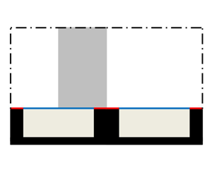
A schematic of the (dimensional) geometry of the parallel-ridge problem is shown in figure 1(a), where a left-handed coordinate system is used. The unidirectional and fully developed flow in the  $z$-direction is driven by a prescribed pressure gradient, $\mathrm {d}p/\mathrm {d}z$, a negative constant. The problem is symmetric in the $x$-direction and the width of the meniscus is $2a$ and that of the ridges is $2(d-a)$. Our domain extends from $x = 0$ to $x = d$ and from $y=0$ to $y=H$, the channel centreline, on account of symmetries. Vapour and/or non-condensable gas may be present in the cavity between the ridges, but we ignore it.

Figure 1. Schematic of the dimensional geometry of the parallel-ridge problem (a) and the corresponding dimensionless geometry (b). The (planar) domain is shown in grey. A (constant) streamwise-pressure gradient is imposed along the  $z$-direction.
2.1. Hydrodynamic problem
The dimensional form of the streamwise-momentum equation is
 \begin{equation} \frac{\partial^{2}w}{\partial x^{2}}+\frac{\partial^{2}w}{\partial y^{2}}=\frac{1}{\mu}\frac{\mathrm{d} p}{\mathrm{d} z}, \end{equation}
where  $w$ is the streamwise velocity and $\mu$ is the dynamic viscosity of the liquid. The shear-free and no-slip boundary conditions along the meniscus and solid–liquid interface, respectively, and symmetry ones elsewhere on the domain manifest themselves as
 $$\begin{gather} \frac{\partial w}{\partial y}=0\quad\mathrm{at}\ y=0\quad \mathrm{for}\ 0< x< a \end{gather}$$
 $$\begin{gather}w=0\quad\mathrm{at}\ y=0\quad \mathrm{for}\ a< x< d \end{gather}$$
 $$\begin{gather}\frac{\partial w}{\partial y}=0\quad\mathrm{at}\ y=H\quad \mathrm{for}\ 0< x< d \end{gather}$$
 $$\begin{gather}\frac{\partial w}{\partial x}=0\quad\mathrm{at}\ x=0\quad\mathrm{and}\quad x=d\quad \mathrm{for}\ 0< y< H, \end{gather}$$
respectively. We non-dimensionalize lengths by  $H$ and indicate that a quantity is non-dimensional by placing a tilde over it. The dimensionless geometry of the problem is shown in figure 1(b). We non-dimensionalize $w$ by $(-\mathrm {d}p/\mathrm {d}z)H^2/(2\mu )$. Then
 \begin{equation} \frac{\partial^{2}\tilde{w}}{\partial\tilde{x}^{2}}+\frac{\partial^{2}\tilde{w}}{\partial\tilde{y}^{2}}={-}2, \end{equation}
subject to
 $$\begin{gather} \frac{\partial\tilde{w}}{\partial\tilde{y}}=0\quad\mathrm{at}\ \tilde{y}=0\quad\mathrm{for}\ 0 < \tilde{x}<\delta\epsilon \end{gather}$$
 $$\begin{gather}\tilde{w}=0\quad\mathrm{at}\ \tilde{y}=0\quad\mathrm{for}\ \delta\epsilon<\tilde{x}<\epsilon \end{gather}$$
 $$\begin{gather}\frac{\partial\tilde{w}}{\partial\tilde{y}}=0\quad\mathrm{at}\ \tilde{y}=1\quad\mathrm{for}\ 0<\tilde{x}<\epsilon \end{gather}$$
 $$\begin{gather}\frac{\partial\tilde{w}}{\partial\tilde{x}}=0\quad\mathrm{at}\ \tilde{x}=0\quad\mathrm{and}\quad \tilde{x}=\epsilon\quad \mathrm{for}\ 0<\tilde{y}<1, \end{gather}$$
where  $\delta =a/d$ is the cavity fraction.
We resolve the velocity field using a matched asymptotic expansion for  $\epsilon \ll 1$ in reference to figure 2(a). The outer region occupies the majority of the domain and it will be shown that, asymptotically, the velocity field there is one-dimensional and parabolic. The spatially periodic portion of the velocity field on account of the ridges is shown to be confined to an inner region in the domain where $\tilde {y}$ is of comparable scale to the ridge pitch.

Figure 2. Depiction of matched asymptotic expansions for flow (a) and temperature (b) problems, where ‘e.s.t.’ denotes exponentially small term.
Our analysis follows that of Hodes et al. (Reference Hodes, Kirk, Karamanis and MacLachlan2017), but both sides rather than one side of the microchannel are textured and thermocapillary stresses along menisci are absent. The extents of the rectangular domain are made independent of the small parameter by working in terms of  $X = \tilde {x}/\epsilon$ such that the problem becomes
 \begin{equation} \frac{1}{\epsilon^{2}}\frac{\partial^{2}\tilde{w}}{\partial X^{2}}+\frac{\partial^{2}\tilde{w}}{\partial\tilde{y}^{2}}={-}2,\end{equation}
subject to
 $$\begin{gather} \frac{\partial\tilde{w}}{\partial\tilde{y}}=0\quad\mathrm{at}\ \tilde{y}=0\quad\mathrm{for}\ 0< X<\delta \end{gather}$$
 $$\begin{gather}\tilde{w}=0\quad\mathrm{at}\ \tilde{y}=0\quad\mathrm{for}\ \delta< X<1 \end{gather}$$
 $$\begin{gather}\frac{\partial\tilde{w}}{\partial\tilde{y}}=0\quad\mathrm{at}\ \tilde{y}=1\quad\mathrm{for}\ 0< X<1 \end{gather}$$
 $$\begin{gather}\frac{\partial\tilde{w}}{\partial X}=0\quad\mathrm{at}\ X=0\quad\mathrm{and}\quad X=1\quad \mathrm{for}\ 0<\tilde{y}<1. \end{gather}$$
2.1.1. Outer region
The outer region of the domain is where  $X=O(1)$, $\tilde {y}=\mathrm {ord}(1)$, i.e. strictly of order unity as $\epsilon \rightarrow 0$. It is sufficiently far from the mixed boundary condition imposed at $\tilde {y}=0$ that the velocity field is one-dimensional, i.e. $\tilde {w} = \tilde {w}(\tilde {y})$, as justified henceforth. Equation (2.11) reduces, to leading order, to $\partial ^{2}\tilde {w}/\partial X^{2}=0$. Integrating, satisfying the symmetry boundary condition in $X$ and integrating again shows that, to leading order, $\tilde {w}=\tilde {w}(\tilde {y})$. Thus, the $\partial ^2\tilde {w}/\partial \tilde {y}^2$ and $-2$ terms in (2.11) balance, implying that $\tilde {w}=O(1)$. We thus, as an ansatz, expand the velocity as a regular power series in $\epsilon$ as per
 \begin{equation} \tilde{w}=\sum_{n=0}^{\infty}\epsilon^{n}\tilde{w}_{n}+ \mathrm{e.s.t.},\quad\epsilon \rightarrow 0,\end{equation}
where  $\tilde {w}_{n}=O(1)$ for all $n\geqslant 0$ and e.s.t. denotes exponentially small terms that are smaller than any algebraic order of $\epsilon$. We do not attempt to solve for these terms, and only include them for error quantification. Substituting (2.16) into (2.11) yields an equation at each (algebraic) order in $\epsilon$ as per
 $$\begin{gather} O\left(\epsilon^{{-}2}\right):\quad \frac{\partial^{2} \tilde{w}_{0}}{\partial X^2}=0 \end{gather}$$
 $$\begin{gather}O\left(\epsilon^{{-}1}\right):\quad \frac{\partial^{2} \tilde{w}_{1}}{\partial X^2}=0 \end{gather}$$
 $$\begin{gather}O\left(\epsilon^{0}\right):\quad \frac{\partial^{2} \tilde{w}_{2}}{\partial X^2}+\frac{\partial^{2} \tilde{w}_{0}}{\partial \tilde{y}^{2}}={-}2 \end{gather}$$
 $$\begin{gather}O\left(\epsilon^{n}\right):\quad \frac{\partial^{2} \tilde{w}_{n+2}}{\partial X^2}+\frac{\partial^{2} \tilde{w}_{n}}{\partial \tilde{y}^{2}}=0,\quad n\geqslant 1. \end{gather}$$
 The symmetry conditions at  $X=0,1$ apply to all orders of $\tilde {w}$. Integrating the $O(\epsilon ^{-1})$ problem and applying them shows that $\tilde {w}_{1}$, like $\tilde {w}_{0}$, is purely a function of $\tilde {y}$. The $O(\epsilon ^{0})$ problem shows that $\partial ^{2}\tilde {w}_{2}/\partial X^{2}$ is purely a function of $\tilde {y}$ and, on account of the symmetry conditions, so is $\tilde {w}_{2}$. By induction in $n$, the remaining problems show that $\tilde {w}_{n}=\tilde {w}{}_{n}(\tilde {y})$ for $n\geqslant 0$. Thus, (2.19)–(2.20) collapse to
 $$\begin{gather} \frac{\mathrm{d}^{2}\tilde{w}_{0}}{\mathrm{d}\tilde{y}^{2}}={-}2 \end{gather}$$
 $$\begin{gather}\frac{\mathrm{d}^{2}\tilde{w}_{n}}{\mathrm{d}\tilde{y}^{2}}=0,\quad n\geqslant 1. \end{gather}$$
Integrating and applying the symmetry condition at the channel centreline as per (2.14) yields
 $$\begin{gather} \tilde{w}_{0}\left(\hat{y}\right)={-}\tilde{y}^{2}+2\tilde{y}+C_{0}, \end{gather}$$
 $$\begin{gather}\tilde{w}_{n}\left(\tilde{y}\right)=C_{n}, \end{gather}$$
where  $C_{n}$ are constants. Thus the solution to the outer problem is
 \begin{equation} \tilde{w}\sim{-}\tilde{y}^{2}+2\tilde{y}+C\left(\epsilon\right)+\mathrm{e.s.t.}, \end{equation}
where
 \begin{equation} C\left(\epsilon\right)=\sum_{n=0}^{\infty}C_{n}\epsilon^{n}.\end{equation}
We turn to the inner problem to satisfy the mixed boundary condition at the composite interface, i.e. the meniscus and the solid–liquid interface.
2.1.2. Inner region
The inner region of the domain is where  $\tilde {x} \sim \tilde {y} =O(\epsilon )$, i.e. they are on the scale of the pitch of the ridges, as $\epsilon \rightarrow 0$. This is sufficiently close to the mixed boundary condition imposed at $\tilde {y}=0$ that the velocity field is two-dimensional, i.e. $\tilde {w} = \tilde {w}(\tilde {x},\tilde {y})$. Our stretched coordinates are $X=\tilde {x}/\epsilon$, $Y=\tilde {y}/\epsilon$ such that the inner region corresponds to $X\sim Y=O(1)$ as $\epsilon \rightarrow 0$ as per figure 2(a). Since the $X$ and $Y$ scales are of the same order, the viscous stress (Laplacian) terms are of the same order in the momentum equation. The velocity scale for the inner problem follows from the outer solution as $\tilde {y}$ is decreased to $O(\epsilon )$. Substituting $\tilde {y}=\epsilon Y$ into (2.25) yields
 \begin{equation} \tilde{w}\sim{-}\epsilon^{2}Y^{2}+2\epsilon Y+C\left(\epsilon\right)+\mathrm{e.s.t.} \end{equation}
Hence, when  $C(\epsilon )=O(1)$, i.e. $C_{0}\neq 0$ as required by (2.11), $\tilde {w}={O(1)}$ in the inner region.
Expressing the inner velocity field as  $\tilde {w}=W(X,Y)$, the problem becomes
 \begin{equation} \frac{\partial^{2}W}{\partial X^{2}}+\frac{\partial^{2}W}{\partial Y^{2}}={-}2\epsilon^{2},\end{equation}
subject to
 $$\begin{gather} \frac{\partial W}{\partial Y}=0\quad \mathrm{at}\ Y=0\quad \mathrm{for}\ 0< X<\delta \end{gather}$$
 $$\begin{gather}W=0\quad \mathrm{at}\ Y=0\quad \mathrm{for}\ \delta< X<1 \end{gather}$$
 $$\begin{gather}W\sim{-}\epsilon^{2}Y^{2}+2\epsilon Y+C(\epsilon)+\mathrm{e.s.t.}\quad \mathrm{as}\ Y\rightarrow\infty\ \mathrm{for}\ 0< X<1 \end{gather}$$
 $$\begin{gather}\frac{\partial W}{\partial X}=0\quad \mathrm{at}\ X=0\quad \mathrm{and}\quad X=1\quad \mathrm{for}\ Y>0, \end{gather}$$
where (2.31) is the (Van Dyke) matching condition. Note that the condition is written as an infinite series here (since  $C(\epsilon )$ is (2.26)) and the inner solution $W$ has not yet been expanded in $\epsilon$, but the matching can be done up to a finite number of terms in the usual way – see Appendix A. Expressing $W$ as
 \begin{equation} W={-}\epsilon^{2}Y^{2}+2\epsilon\hat{W},\end{equation} $\hat {W}$ must satisfy
 \begin{equation} \nabla^{2}\hat{W}=0, \end{equation}
subject to
 $$\begin{gather} \frac{\partial\hat{W}}{\partial Y}=0\quad\mathrm{at}\ Y=0\quad\mathrm{for}\ 0< X<\delta \end{gather}$$
 $$\begin{gather}\hat{W}=0\quad\mathrm{at}\ Y=0\quad\mathrm{for}\ \delta< X<1 \end{gather}$$
 $$\begin{gather}\hat{W}\sim Y+\frac{C\left(\epsilon\right)}{2\epsilon}+\mathrm{e.s.t.}\quad\mathrm{as}\ Y\rightarrow\infty \end{gather}$$
 $$\begin{gather}\frac{\partial\hat{W}}{\partial X}=0\quad\mathrm{at}\ X=0\quad\mathrm{and}\quad X=1\quad\mathrm{for}\ 0< Y<\infty. \end{gather}$$
This  $\hat {W}$ problem is the superposition of a one-dimensional linear-shear flow over a smooth surface and a perturbation to it which accommodates a mixed boundary condition and manifests itself with a constant mean velocity over the width of the domain. It has been solved using a conformal map by Philip (Reference Philip1972a,Reference Philipb). The solution up to the exponentially small error in the matching condition is
 \begin{equation} \hat{W}={\rm Im}\left\{ \frac{2}{\rm \pi}\cos^{{-}1}\left[\frac{\mathrm{cos}\left({\rm \pi} \varTheta_{{\parallel}}/2\right)}{\cos\left({\rm \pi}\delta/2\right)}\right]\right\}+\mathrm{e.s.t.}, \end{equation}
where  $\varTheta _{\parallel }=X+\mathrm {i}Y$, and
 \begin{equation} \hat{W}\sim Y+\lambda+\mathrm{e.s.t.}\quad\mathrm{as}\ Y\rightarrow\infty, \end{equation}
where
 \begin{equation} \lambda=\frac{2}{\rm \pi}\ln[\mathrm{sec}\left(\delta{\rm \pi}/2\right)].\end{equation}
It follows that
 \begin{equation} C\left(\epsilon\right)=2\epsilon \lambda\end{equation}
and the inner and outer solutions are
 \begin{gather} W\sim\overbrace{2\,{\rm Im}\left\{ \frac{2}{\rm \pi}\cos^{{-}1}\left[\frac{\cos\left({\rm \pi} \varTheta_{{\parallel}}/2\right)}{\mathrm{cos}\left({\rm \pi}\delta/2\right)}\right]\right\}}^{W_1}\epsilon+\overbrace{({-}Y^{2})}^{W_2}\epsilon^{2}+\mathrm{e.s.t.} \end{gather}
 \begin{gather}\tilde{w}\sim \overbrace{-\tilde{y}^{2} +2\tilde{y}}^{\tilde{w}_0}+\overbrace{2\lambda}^{\tilde{w}_1}\epsilon+\mathrm{e.s.t.}, \end{gather}
respectively. Note that we did not have to expand  $W$ (or $\hat {W}$) in powers of $\epsilon$ to arrive at the above inner solution and it has been checked that matching order by order (as in Appendix A) gives the same result.
2.1.3. Composite solution
The solutions for the inner and outer regions are in agreement in the overlap region, where the outer one keeps its form. Therefore, the inner solution, (2.43), which is accurate to all algebraic orders in  $\epsilon$, is uniformly valid throughout the domain, i.e. it is the composite solution as per, in outer variables,
 \begin{equation} \tilde{w}_{comp}\sim{-}\tilde{y}^2 +2\epsilon\,{\rm Im}\left\{\frac{2}{\rm \pi}\cos^{{-}1}\left[\frac{\cos\left({\rm \pi} \left(\tilde{x}/\epsilon + \mathrm{i}\tilde{y}/\epsilon\right)/2\right)}{\cos\left({\rm \pi}\delta/2\right)}\right]\right\}+\mathrm{e.s.t}. \end{equation}
2.1.4. Slip length
The slip length quantifies the flow enhancement provided by texturing a microchannel with a SH surface(s). It is related to the one-dimensional (Navier-slip) problem, which does not resolve the local velocity field in the inner region, and is governed by
 \begin{equation} \frac{\mathrm{d}^2 \tilde{w}_{{1d}}}{\mathrm{d} \tilde{y}^2}={-}2, \end{equation}
where  ${\tilde {w}_{1{d}}}$ is the dimensionless velocity averaged over a ridge period. It is subject to the symmetry condition at $\tilde {y} = 1$ and a Navier-slip boundary condition on the SH surface as per
 \begin{equation} \tilde{w}_{1{d},\tilde{y}=0}=\tilde{b}\left.\frac{\mathrm{d}\tilde{w}_{{1d}}}{\mathrm{d} \tilde{y}}\right|_{\tilde{y}=0}, \end{equation}
where
 \begin{equation} \tilde{b}=\frac{b}{h}, \end{equation}
is the dimensionless slip length. It follows that
 \begin{equation} \tilde{w}_{{1d}}={-}\tilde{y}^2+2\tilde{y}+2\tilde{b}, \end{equation}
and its mean value is
 \begin{equation} \bar{\tilde{w}}_{{1d}}=2\tilde{b} +\tfrac{2}{3}. \end{equation}
 Following Lauga & Stone (Reference Lauga and Stone2003), we compute the slip length by equating the mean velocities from the composite and one-dimensional (Navier-slip) velocity profiles. As with the flow configurations resolved by Philip (Reference Philip1972a,Reference Philipb), the velocity field for our configuration is the sum of that for a one-dimensional, Poiseuille flow in a microchannel with smooth walls and a velocity-increment field. The latter is not subject to any forcing term and obeys the shear-free boundary condition at  $\tilde {y}=1$. Therefore, there is no net momentum transferred across any plane normal to the composite interface in the velocity-increment problem and thus the mean velocity increment over the width of the domain is a constant, i.e. $2\epsilon \lambda +\mathrm {e.s.t.}$ Thus, the outer solution is valid throughout the domain insofar as computing the slip length and it follows from (2.25), (2.42) and (2.49) that
 \begin{equation} \tilde{b}\sim \epsilon \lambda+\mathrm{e.s.t}. \end{equation}
2.1.5. Discussion
We utilized a matched asymptotic expansion to develop the preceding hydrodynamic results, as done by Hodes et al. (Reference Hodes, Kirk, Karamanis and MacLachlan2017), Kirk (Reference Kirk2018) and Kirk et al. (Reference Kirk, Karamanis, Crowdy and Hodes2020), and they facilitate the below solution of the thermal problem. Teo & Khoo (Reference Teo and Khoo2009) obtained it by taking the limit as  $\epsilon \rightarrow 0$ of the dual-series equations satisfying the mixed boundary condition and their numerical solutions of them accommodate arbitrary values of $\epsilon$ and $\delta$. Kirk et al. (Reference Kirk, Hodes and Papageorgiou2017) too showed that the error in our result is exponentially small. More recently, Marshall (Reference Marshall2017) obtained an exact formula for the slip length (expressed as contour integrals) for arbitrary $\epsilon$ and $\delta$ and, additionally, weakly curved menisci, by using conformal maps, loxodromic function theory and reciprocity arguments. Additional effects have been considered by many investigators. For example, Kirk (Reference Kirk2018) relaxed the assumption of weakly curved menisci in the large solid fraction limit for $\epsilon \ll 1$. Moreover, in numerical studies, Game et al. (Reference Game, Hodes, Keaveny and Papageorgiou2017) captured edge and subphase effects and Game, Hodes & Papageorgiou (Reference Game, Hodes and Papageorgiou2019) captured inertial effects due to slowly varying curvature along a shear-free meniscus on account of the pressure difference across the meniscus decreasing in the streamwise direction.
We note that, when the microchannel is textured on only one side, the same analysis done by Hodes et al. (Reference Hodes, Kirk, Karamanis and MacLachlan2017) yields the composite velocity profile as
 \begin{equation} \tilde{w}_{comp}\sim{-}\tilde{y}^2 +\frac{\epsilon}{1+\epsilon \lambda} {\rm Im}\left\{\frac{2}{\rm \pi}\cos^{{-}1}\left[\frac{\cos\left({\rm \pi} \left(\tilde{x}/\epsilon + \mathrm{i}\tilde{y}/\epsilon\right)/2\right)}{\cos\left({\rm \pi}\delta/2\right)}\right]\right\} +\mathrm{e.s.t}. \end{equation}
Also, an exact solution based on a (cumbersome) conformal map is available for this case (Philip Reference Philip1972a,Reference Philipb) and comparison with it shows that the composite velocity profile and corresponding slip length are accurate to  $O(\mathrm {e}^{-{\rm \pi} /\epsilon })$ (Hodes et al. Reference Hodes, Kirk, Karamanis and MacLachlan2017), confirming that the error is exponentially small. In the symmetric microchannel case at hand, there are no higher-order ( $O(\epsilon ^3)$) algebraic terms and hence the $O(\epsilon ^2)$ term could be expected in (2.43) (although the fact that the next term is exponentially small is unexpected). If the channel is not symmetric but textured only on one wall as in (2.52) (or instead has curved menisci – see Kirk Reference Kirk2018), then an expansion for $\epsilon \ll 1$ shows that all algebraic orders are present in the hydrodynamics.
2.2. Thermal problem
2.2.1. Formulation
The dimensional form of the thermal energy equation is
 \begin{equation} w\frac{\partial T}{\partial z}=\alpha\left(\frac{\partial^{2}T}{\partial x^{2}}+\frac{\partial^{2}T}{\partial y^{2}}\right),\end{equation}
where axial conduction is absent because the temperature field is fully developed and  $\alpha =k/(\rho c_{p})$ is the thermal diffusivity of the liquid, where $k$ is its thermal conductivity, $\rho$ is its density and $c_{p}$ is its specific heat at constant pressure. The boundary conditions on (2.53) are
 $$\begin{gather} \frac{\partial{T}}{\partial{y}}=0\quad\mathrm{at}\ {y}=0\quad\mathrm{for}\ 0<{x}< a \end{gather}$$
 $$\begin{gather}\frac{\partial{T}}{\partial{y}}={-}\frac{q''_{sl}}{k}\quad\mathrm{at}\ {y}=0\quad\mathrm{for}\ a<{x}< d \end{gather}$$
 $$\begin{gather}\frac{\partial{T}}{\partial{y}}=0\quad\mathrm{at}\ {y}=H\quad\mathrm{for}\ 0<{x}< d \end{gather}$$
 $$\begin{gather}\frac{\partial{T}}{\partial{x}}=0\quad\mathrm{at}\ {x}=0\quad\mathrm{and}\quad{x}=a\quad\mathrm{for}\ 0<{y}< H, \end{gather}$$
where  $q''_{sl}$ is the (constant) heat flux prescribed along the solid–liquid interface. Moreover, again, because of the thermally fully developed assumption, along with the constant heat flux boundary condition, we have
 \begin{equation} \frac{\partial T}{\partial z}=\frac{q_{sl}''(d-a)}{Q\rho c_{p}}, \end{equation}
where  $Q$ is the volumetric flow rate of liquid through a half-period.
Henceforth, we proceed with the non-dimensional form of the problem, where temperature is non-dimensionalized (in a similar way as was done by Kirk et al. Reference Kirk, Hodes and Papageorgiou2017) by subtracting the (bulk) mean liquid temperature,  $T_{m}$, and dividing by a characteristic temperature scale of $q_{sl}''H/k$ such that
 \begin{equation} \tilde{T}=\frac{k\left(T-T_{m}\right)}{q_{sl}''H}, \end{equation}
where
 \begin{equation} T_{m}=\frac{\displaystyle\int\nolimits_0^H \int_0^dwT\,\mathrm{d}\,x\,\mathrm{d}y}{\displaystyle\int\nolimits_0^H \int_0^dw\,\mathrm{d}\,x\,\mathrm{d}y}.\end{equation}
The thermal energy equation becomes
 \begin{equation} \frac{\epsilon \phi}{\tilde{Q}}\tilde{w}=\frac{\partial^{2}\tilde{T}}{\partial\tilde{x}^{2}}+\frac{\partial^{2}\tilde{T}}{\partial\tilde{y}^{2}}, \end{equation}
where  $\phi =1-\delta$ is the solid fraction of the ridges and $\tilde {Q} = 2\mu Q/[(-\mathrm {d}p/\mathrm {d}z) H^4]$. The forcing term, $\epsilon \phi \tilde {w}/\tilde {Q}$, is known (to all algebraic orders) from the solution to the hydrodynamic problem.
Noting that
 \begin{equation} \tilde{Q}\sim \left(2\epsilon \lambda +2/3\right)\epsilon+\mathrm{e.s.t.},\quad\epsilon \rightarrow 0, \end{equation}
the dimensionless thermal energy equation (written in terms of  $X$ such that the domain boundaries are independent of $\epsilon$) becomes
 \begin{equation} \frac{\phi}{2/3+2\epsilon \lambda}\tilde{w}+\mathrm{e.s.t.}=\frac{1}{\epsilon^{2}}\frac{\partial^{2}\tilde{T}}{\partial X^{2}}+\frac{\partial^{2}\tilde{T}}{\partial\tilde{y}^{2}},\end{equation}
subject to
 $$\begin{gather} \frac{\partial{\tilde{T}}}{\partial{\tilde{y}}}=0\quad\mathrm{at}\ \tilde{y}=0\quad\mathrm{for}\ 0<{X}<\delta \end{gather}$$
 $$\begin{gather}\frac{\partial{T}}{\partial{\tilde{y}}}={-}1\quad\mathrm{at}\ \tilde{y}=0\quad\mathrm{for}\ \delta<{X}< 1 \end{gather}$$
 $$\begin{gather}\frac{\partial\tilde{T}}{\partial\tilde{y}}=0\quad\mathrm{at}\ \tilde{y}=1\quad\mathrm{for}\ 0<{X}<1 \end{gather}$$
 $$\begin{gather}\frac{\partial\tilde{T}}{\partial{X}}=0\quad\mathrm{at}\ {X}=0\quad\mathrm{and}\quad X=1. \end{gather}$$
2.2.2. Outer region
The forcing term in the above problem is  $O(1)$ and thus, by the same reasoning used to justify that $\tilde {w} =\tilde {w}(\tilde {y}) = O(1)$, we also have $\tilde {T}=\tilde {T}(\tilde {y}) = O(1)$ to leading order. We thus expand the temperature field as
 \begin{equation} \tilde{T}=\sum_{n=0}^{\infty}\epsilon^{n}\tilde{T}_{n}+\mathrm{e.s.t.},\quad\epsilon \rightarrow 0,\end{equation}
where  $\tilde {T}_{n}=O(1)$ for all $n\geqslant 0$.
Substituting (2.68) and the solution for the outer velocity profile as per (2.44) into (2.63), we find that, at the various orders of  $\epsilon$,
 $$\begin{gather} O(\epsilon^{{-}2}):\quad\frac{\partial^{2} \tilde{T}_{0}}{\partial X^2}=0 \end{gather}$$
 $$\begin{gather}O(\epsilon^{{-}1}):\quad\frac{\partial^{2} \tilde{T}_{1}}{\partial X^2}=0 \end{gather}$$
 $$\begin{gather}O(\epsilon^{0}):\quad\frac{\partial^{2} \tilde{T}_{2}}{\partial X^2}+ \frac{\partial^{2} \tilde{T}_{0}}{\partial \tilde{y}^{2}}=\frac{3\phi}{2}\left(-\tilde{y}^{2}+2\tilde{y}\right) \end{gather}$$
 $$\begin{gather}O(\epsilon^{n}):\quad\frac{\partial^{2} \tilde{T}_{n+2}}{\partial X^2}+ \frac{\partial^{2} \tilde{T}_{n}}{\partial \tilde{y}^{2}}=\frac{3\phi}{2}[ ({-}3\lambda)^n(-\tilde{y}^2+2\tilde{y})+({-}3\lambda)^{n-1}2\lambda],\quad n\geqslant 1. \end{gather}$$
Following the same approach as in the outer hydrodynamic problem shows that  $\tilde {T}_{n}=\tilde {T}{}_{n}(\tilde {y})$ for all $n$. The solution to the outer problem, which satisfies all 3 symmetry conditions, follows as
 \begin{equation} \tilde{T}=\frac{\phi}{2/3+2\epsilon \lambda}\left[-\frac{\left(\tilde{y}-1\right)^{4}}{12}+\left(\frac{1}{2}+\epsilon \lambda\right)\left(\tilde{y}-1\right)^{2}+D\left(\epsilon\right)\right] +\mathrm{e.s.t.},\quad\epsilon \rightarrow 0, \end{equation}
where
 \begin{equation} D(\epsilon)=\sum_{n=0}^{\infty}\epsilon^{n}D_{n}. \end{equation}
2.2.3. Inner region
Denoting the inner temperature profile as  $\tilde {T}=\theta (X,Y)$, the thermal energy equation becomes
 \begin{align} \frac{\partial^{2}\theta}{\partial X^{2}}+\frac{\partial^{2}\theta}{\partial Y^{2}}=\frac{\phi}{2/3+2\epsilon \lambda}\left(-\epsilon^{4}Y^2+2\epsilon^{3}{\rm Im}\left\{ \frac{2}{\rm \pi}\cos^{{-}1}\left[\frac{\cos\left({\rm \pi} Z/2\right)}{\cos\left({\rm \pi}\delta/2\right)}\right]\right\} \right)+\mathrm{e.s.t.}\end{align}
The forcing is  $O(\epsilon ^{3})$; therefore, neglecting terms of this order, it reduces to Laplace's equation as per
 \begin{equation} \frac{\partial^{2}\theta}{\partial X^{2}}+\frac{\partial^{2}\theta}{\partial Y^{2}}= O\left(\epsilon^3\right), \end{equation}
subject to
 \begin{gather} \frac{\partial\theta}{\partial Y}=0\quad\mathrm{at}\ Y=0\quad\mathrm{for}\ 0< X<\delta \end{gather}
 \begin{gather}\frac{\partial\theta}{\partial Y}={-}\epsilon\quad\mathrm{at}\ Y=0\quad\mathrm{for}\ \delta< X<1 \end{gather}
 \begin{gather}\theta\sim{-}\epsilon\phi Y+\phi\left[\frac{1}{2}+\frac{1/12+D(\epsilon)}{2/3+2\epsilon \lambda}\right]+O \left(\epsilon^{3}\right)\quad\mathrm{as}\ Y\rightarrow\infty \end{gather}
 \begin{gather}\frac{\partial\theta}{\partial X}=0\quad\mathrm{at}\ X=0\quad\mathrm{and}\quad X=1\quad\mathrm{for}\ Y>0, \end{gather}
where (2.79), which follows from (2.73) with  $\tilde {y} = \epsilon Y$, is the matching condition. As per the solution by Mikic (Reference Mikic1957) to this problem in the context of (thermal) spreading resistance
 \begin{align} \theta ={-}\epsilon \phi Y - \frac{2\epsilon}{{\rm \pi}^2}\sum_{n=1}^{\infty}\frac{\sin\left(n{\rm \pi}\delta\right)\cos\left(n{\rm \pi} X\right)\mathrm{e}^{{-}n {\rm \pi}Y}}{n^2}+\phi\left[\frac{1}{2}+\frac{1/12+D(\epsilon)}{2/3+2\epsilon \lambda}\right]+O\left(\epsilon^{3}\right). \end{align}
We solve for  $D(\epsilon )$ by enforcing that the dimensionless mean liquid temperature, as defined by (2.59) and (2.60), is zero, i.e. using outer variables
 \begin{equation} \int_{0}^{1}\int_0^{\epsilon}\tilde{w}\tilde{T}\,\mathrm{d}\,\tilde{x}\,\mathrm{d}\tilde{y}=0. \end{equation}
In Appendix B, we show that we can enforce this condition using the outer solutions only, up to an error of  $O(\epsilon ^3)$, and the final temperature along the composite interface is found to be
 \begin{equation} \theta \left(X,0\right) = \phi \hat{D}\left(\epsilon \lambda\right) - \frac{2\epsilon}{{\rm \pi}^2}\sum_{n=1}^{\infty}\frac{\sin\left(n{\rm \pi}\delta\right)\cos\left(n{\rm \pi} X\right)}{n^2}+O\left(\epsilon^{3}\right), \end{equation}
where  $\hat {D}(\epsilon \lambda )$ (which is related to $D(\epsilon )$) is given by the explicit formula (B9).
2.2.4. Composite solution
The inner solution is not the composite one as in the hydrodynamic problem because (2.79) is consistent with (2.73) only up to  $O(\epsilon ^2)$. Rather
 \begin{equation} \tilde{T}_{comp} = \tilde{T}_{out} + \tilde{T}_{in} - \tilde{T}_{overlap}; \end{equation}
consequently
 \begin{align} \tilde{T}_{comp} &\sim \frac{\phi}{\dfrac{2}{3}+2\epsilon \lambda}\left[-\frac{\left( \tilde{y}-1\right)^{4}}{12}+\left(\frac{1}{2}+\epsilon \lambda\right)\left(\tilde{y}-1\right)^{2}+ \breve{D}\left(\epsilon\right)\right]\nonumber\\ &\quad - \frac{2\epsilon}{{\rm \pi}^2}\sum_{n=1}^{\infty}\frac{\sin\left(n{\rm \pi}\delta\right)\cos\left(n{\rm \pi} \dfrac{\tilde{x}}{\epsilon}\right)\exp\left({-n {\rm \pi}\dfrac{\tilde{y}}{\epsilon}}\right)} {n^2}+O\left(\epsilon^3\right). \end{align}
2.2.5. Nusselt numbers
We define the local Nusselt number along the solid–liquid interface as
 \begin{equation} {Nu}(X) = \frac{4h(X)H}{k}, \end{equation}
where  $h(X)$ is the (local) heat transfer coefficient, i.e. $q''_{sl}/(T_{sl}-T_{m})$, which is finite along the solid–liquid interface and zero along the meniscus. Then
 \begin{equation} {Nu}(X) = \begin{cases} 0 & \mathrm{for}\ 0\leqslant X < \delta\\ \dfrac{4}{\theta\left(X,0\right)} & \mathrm{for}\ \delta < X \leqslant 1. \end{cases} \end{equation}
The minimum local Nusselt number ( ${Nu_{min}}$) occurs at the centre of a ridge, i.e. $X=1$, as per
 \begin{equation} {Nu_{min}} = \frac{4}{\theta\left(1,0\right)}. \end{equation}
This is an important engineering parameter because the magnitude of the maximum temperature difference between the ridge and bulk liquid follows from it. From (2.83), the minimum local Nusselt number ( ${Nu_{min}}$) may be expressed as
 \begin{equation} {Nu_{min}} = \frac{4}{ \phi \left[ \hat{D}\left(\epsilon \lambda\right)+\dfrac{2\epsilon}{\phi} \sum_{n=1}^{\infty}\dfrac{\sin\left(n{\rm \pi}\phi\right)}{\left(n{\rm \pi}\right)^2}\right]}+O\left(\epsilon^{3}\right). \end{equation}
More generally, the local Nusselt number anywhere along the ridge is
 \begin{align} {Nu}(X) = \frac{4}{ \phi \left( \hat{D}\left(\epsilon \lambda\right) - \dfrac{2\epsilon}{\phi} \sum_{n=1}^{\infty}\dfrac{\sin\left(n{\rm \pi}\delta\right)\cos\left(n{\rm \pi} X\right)}{n^2{\rm \pi}^2}\right) }+O\left(\epsilon^{3}\right), \quad \delta < X \leqslant 1. \end{align}
This was derived in the limit of small  $\epsilon$, but the subsequent behaviour in the small solid fraction limit, $\phi \to 0$, is also of interest. This limit is physically relevant, but care should be taken when making further approximations in $\epsilon$ that the correct asymptotic behaviour in the secondary limit $\phi \to 0$ is preserved. If it is not preserved, e.g. if one simply expands (2.90) directly in powers of $\epsilon$, the accuracy and validity of such an expression is significantly reduced. This is elucidated in Appendix C, where we instead expand in powers of $\mathcal {E}(\epsilon )= \epsilon / (\hat {D} + \epsilon \lambda )$, yielding
 \begin{align} {Nu}(X) &= \frac{4}{\phi \left[\hat{D}\left(\epsilon \lambda\right)+\epsilon \lambda\right]} \left\{1+ \mathcal{E}(\epsilon)\left[ \lambda+S(X)\right] + \mathcal{E}(\epsilon)^2\left[\lambda+S(X)\right]^2\right\} \nonumber\\ &\quad + O\left(\epsilon^3\right)\quad \mathrm{for}\ \delta < X \leqslant 1. \end{align}
The quantity  $\mathcal {E}$ remains bounded even if $\phi \to 0$, and hence the expansion stays well ordered. The $O(\epsilon ^3)$ error term accounts for the $O(\mathcal {E}^3)$ terms since $\mathcal {E} = O(\epsilon )$. We note that, by evaluating Nu in the limit when the solid fraction is 1, i.e. for a smooth channel such that $\lambda \rightarrow 0$, we recover the well-known result that $Nu = 140/17$. (The $O(\epsilon ^3)$ error term can be shown to vanish in this limit.)
The average Nusselt number for the composite interface is defined in the manner of Maynes & Crockett (Reference Maynes and Crockett2014) and Kirk et al. (Reference Kirk, Hodes and Papageorgiou2017) as
 \begin{equation} \overline{Nu} = \frac{4\bar{h}H}{k}, \end{equation}
where  $\bar {h} = \int _a^d h\,\mathrm {d}\,x/d$. Thus
 \begin{equation} \overline{Nu}=\int_{\delta}^{1}{Nu}(X)\,\mathrm{d}X. \end{equation}
Performing the integration on (2.91), and substituting the series  $S(X)$, we find that
 \begin{align} \overline{Nu} &\sim \frac{4}{\hat{D}\left(\epsilon \lambda\right)+\epsilon \lambda}\left\{ 1+\left[\lambda-\sum_{n=1}^{\infty}\frac{2\sin^2\left(n{\rm \pi}\delta\right)}{\phi^2\left(n{\rm \pi}\right)^3} \right]\mathcal{E}(\epsilon)\right. \nonumber\\ &\quad \left.+ \left[\lambda^2-2\lambda\sum_{n=1}^{\infty}\frac{2\sin^2\left(n{\rm \pi}\delta\right)}{\phi^2\left(n{\rm \pi}\right)^3}+\sum_{m=1}^{\infty}\sum_{n=1}^{\infty}L_{m,n}\right]\mathcal{E}(\epsilon)^2\right\} +O\left(\epsilon^3\right), \end{align}
where
 \begin{align} L_{mn} = \frac{4}{\phi^3}\frac{\sin\left(n{\rm \pi}\delta\right) \sin\left(m{\rm \pi}\delta\right)}{\left(n{\rm \pi}\right)^2\left(m{\rm \pi}\right)^2} \begin{cases} \dfrac{1}{2}\left[1-\delta - \dfrac{\sin\left(2n{\rm \pi}\delta\right)}{2n{\rm \pi}}\right] & \mathrm{for}\ m=n\\[10pt] -\dfrac{\sin\left[\left(m+n\right){\rm \pi}\delta\right]}{2{\rm \pi}\left(m+n\right)} - \dfrac{\sin\left[\left(m-n\right){\rm \pi}\delta\right]}{2{\rm \pi}\left(m-n\right)} & \mathrm{for}\ m \neq n. \end{cases} \end{align}
Alternatively, a simpler expression valid for any solid fraction with no sums to evaluate, but with an  $O(\epsilon )$ error term, follows from the leading term of (2.94)
 \begin{equation} \overline{Nu} \sim \frac{4}{\hat{D}\left(\epsilon \lambda\right)+\epsilon \lambda} + O\left(\epsilon\right). \end{equation}
An average Nusselt number may also be defined in the manner of Enright et al. (Reference Enright, Hodes, Salamon and Muzychka2014) as
 \begin{equation} \overline{Nu}' =\frac{4\bar{h}'H}{k}, \end{equation}
by defining the average heat transfer coefficient as  $\bar {h}'= \phi q''_{sl}/(\overline {T_{sl}-T_{m}})$ such that it is based upon the mean heat flux over the composite interface ( $\phi q''_{sl}$) and the mean driving force for heat transfer over the solid–liquid one ( $\overline {T_{sl}-T_{m}}$). Then, it is given by
 \begin{equation} \overline{Nu}' = \frac{4\phi^2}{\displaystyle\int\nolimits_{\delta}^1 \theta \left(X,0\right) \mathrm{d}X}. \end{equation}
Performing the integration we find that
 \begin{align} \overline{Nu}'&= 140\left(1+3\epsilon \lambda\right)^2\left/\left\{ 17+ \left[84\lambda + \frac{70}{\phi^2{\rm \pi}^3}\sum_{n=1}^{\infty}\frac{\sin^2\left(n{\rm \pi}\delta\right)}{n^3}\right]\epsilon \right. \right. \nonumber\\ &\quad \left. +\left[ 105\lambda^2 +\frac{420\lambda}{\phi^2{\rm \pi}^3}\sum_{n=1}^{\infty}\frac{\sin^2\left(n{\rm \pi}\delta\right)}{n^3} \right]\epsilon^2+\left[ \frac{630\lambda^2}{\phi^2{\rm \pi}^3}\sum_{n=1}^{\infty}\frac{\sin^2\left(n{\rm \pi}\delta\right)}{n^3}\right]\epsilon^3\right\} +O\left(\epsilon^3\right). \end{align}
There is no need to expand this result further in  $\epsilon$, and it also vanishes as expected when $\lambda \rightarrow \infty$ (i.e. $\phi \rightarrow 0$). Also, the last term in the denominator is retained as, depending on the relative values of $\lambda$ and $\epsilon$, it may contribute significantly to the result. Finally, we note that, regardless of which definition of the mean Nusselt number is used, the local one is given by (2.86). In Appendix D, we validate the asymptotic behaviour of this result against the exact solution of Kirk et al. (Reference Kirk, Hodes and Papageorgiou2017).
2.2.6. Prior results
The prior studies by Maynes & Crockett (Reference Maynes and Crockett2014) and Kirk et al. (Reference Kirk, Hodes and Papageorgiou2017) provide the local Nusselt number as per (2.86) and, by implication, the minimum one as per (2.88), as well as the mean Nusselt Number  $\overline {Nu}$ as per (2.92). The mean Nusselt number $\overline {Nu}'$ as per (2.97) also follows from the temperature profiles developed in these studies. Moreover, the studies by Enright et al. (Reference Enright, Eason, Dalton, Hodes, Salamon, Kolodner and Krupenkin2006) and Enright et al. (Reference Enright, Hodes, Salamon and Muzychka2014) provide $\overline {Nu}'$ and machinery that may be adopted to find the local Nusselt numbers. We proceed to discuss and contrast all of them and our own results.
Maynes & Crockett (Reference Maynes and Crockett2014) used a Navier-slip velocity profile in the thermal energy equation. An analytical solution for the temperature profile was found by representing the discontinuous (Neumann) boundary condition along the composite interface as a Fourier series and using separation of variables. Their temperature profile (in our notation) along the composite interface is
 \begin{align} \theta_{M}\left(X,0\right) &= \frac{17}{35}\phi -\frac{2\epsilon}{{\rm \pi}^2}\sum_{n=1}^{\infty}\frac{\sin\left(n{\rm \pi}\delta\right)\coth\left(n{\rm \pi}/\epsilon\right) \cos\left(n{\rm \pi} X\right)}{n^2} -\frac{18}{35}\frac{\phi \epsilon \lambda}{1+3\epsilon \lambda}\nonumber\\ &\quad +\frac{6}{35}\frac{\phi\epsilon^2 \lambda^2}{\left(1+3\epsilon \lambda\right)^2}, \end{align}
where the subscript ‘M’ denotes a result by Maynes & Crockett (Reference Maynes and Crockett2014). Closed-form expressions for  ${Nu}_{M}$ and ${Nu}_{{min,M}}$ follow and their behaviour is discussed by Maynes & Crockett (Reference Maynes and Crockett2014). A closed-form expression for $\overline {Nu}'_{M}$ also follows from integrating (2.100). Numerical integration was used by Maynes & Crockett (Reference Maynes and Crockett2014) to compute $\overline {Nu}_{M}$. Although Maynes & Crockett (Reference Maynes and Crockett2014) did not quantify the error in their Nusselt number expressions due to using a Navier-slip velocity profile, we have shown that it is $O(\epsilon ^3)$. Relatedly, upon noting that $\coth (n{\rm \pi} /\epsilon ) \sim 1 + \mathrm {e.s.t.}$ as $\epsilon \rightarrow 0$, an expansion of (2.100) is consistent with (2.83) and all of the Nusselt numbers become the same as in our analysis. We note, however, that, since Maynes & Crockett (Reference Maynes and Crockett2014) did not do this, their results differ slightly from ours.
Insofar as  $\overline {Nu}'$, Enright et al. (Reference Enright, Eason, Dalton, Hodes, Salamon, Kolodner and Krupenkin2006) were the first to compute it and, as here, solid–liquid interfaces were isoflux. They too utilized a Navier-slip velocity profile as per (2.50), or the corresponding expression when one side of the microchannel is textured, but did not capture the discontinuous thermal boundary condition along the composite interface. Consequently, the Nusselt number was solely dependent upon the slip length non-dimensionalized by the channel height for the texture of interest (parallel or transverse ridges, pillars, etc.). Enright et al. (Reference Enright, Hodes, Salamon and Muzychka2014) refined this approach by further imposing an apparent temperature jump along the composite (c) interfaces on one or both sides of a microchannel as per
 \begin{equation} \bar{T}_{sl} - \bar{T}_{c} ={-}b_{t} \left.\frac{\partial \bar{T}}{\partial n}\right|_{c}, \end{equation}
where  $b_{t}$ is the apparent thermal slip length (also referred to as the temperature jump length) and $n$ the direction normal to a composite interface and pointing into the liquid. Using the approach of Nield (Reference Nield2004, Reference Nield2008) to accommodate asymmetrical boundary conditions, closed-form expressions for the Nusselt number were developed as a function of arbitrary values of $b$ and $b_{t}$ imposed on each side of the microchannel and, additionally, the ratio of heat fluxes averaged over the composite interfaces ( $\phi q''_{sl}$) bounding the domain (liquid). In the case of a symmetric channel, as in this study, the results by Enright et al. (Reference Enright, Hodes, Salamon and Muzychka2014) reduce to those developed by Inman (Reference Inman1964) 50 years earlier in the context of molecular slip effects in gas flows, where the surface boundary conditions are mathematically equivalent. Kane & Hodes (Reference Kane and Hodes2019) extended the Enright et al. (Reference Enright, Hodes, Salamon and Muzychka2014) analysis to a combined Poiseuille and Couette flow.
The (one-dimensional) temperature field provided by the foregoing studies in the case of parallel ridges is that averaged over the width of the domain. Insofar as the definition of dimensionless temperature adopted here as per (2.59), only the composite interface temperature is relevant; consequently, the thermal slip length is irrelevant. The resulting temperature profile, which we denote by  $\tilde {T}_{E}$, is
 \begin{align} \tilde{T}_{E} = \frac{\phi}{2/3+2\epsilon \lambda}\left( -\frac{\tilde{y}^4}{12} + \frac{\tilde{y}^3}{3} + \epsilon \lambda \tilde{y}^2 -2\epsilon \lambda \tilde{y} - \frac{2}{3} \tilde{y} +\frac{2}{105}\frac{17+84\epsilon \lambda + 105 \epsilon^2 \lambda^2}{1+3\epsilon \lambda} \right). \end{align}
This expression is identical to that given by (2.73) with  $D(\epsilon )$ given by (B7). Terms of $O(\epsilon ^3)$ were neglected in our derivation and thus, albeit not pointed out by Enright et al. (Reference Enright, Hodes, Salamon and Muzychka2014), it is only accurate to $O(\epsilon ^3)$.
In the foregoing studies (except in Enright et al. Reference Enright, Eason, Dalton, Hodes, Salamon, Kolodner and Krupenkin2006), the difference between the mean temperatures of the solid–liquid and composite interfaces follows by imposing an apparent thermal slip boundary condition as per (2.101). Enright et al. (Reference Enright, Hodes, Salamon and Muzychka2014) utilized the spreading resistance solution by Mikic (Reference Mikic1957) to evaluate  $b_{t}$ such that
 \begin{equation} b_{t}=\frac{2d}{{\rm \pi}^3\phi^2} \sum_{n=1}^{\infty} \frac{\sin^2\left(n{\rm \pi}\phi\right)}{n^3}. \end{equation}
The Nusselt number  $\overline {Nu}'_{E}$, where the subscript ‘E’ indicates a result from Enright et al. (Reference Enright, Hodes, Salamon and Muzychka2014), then follows from the definition of the bulk temperature and it does not capture the error term as in the present analysis. Consequently, the relationship between the present result and that by Enright et al. (Reference Enright, Hodes, Salamon and Muzychka2014) is
 \begin{equation} \overline{Nu}'=\overline{Nu}'_{E} + O(\epsilon^3). \end{equation}
 Replacing  $b_{t}$ in the Enright et al. (Reference Enright, Hodes, Salamon and Muzychka2014) analysis with its maximum value, $b_{{t,max}}$, to define the apparent temperature jump along the composite interface in terms of the temperature of the centre of the ridge, (2.103) becomes
 \begin{equation} T_{sl}\left(x=d\right) - \bar{T}_{c} ={-}b_{{t,max}} \left.\frac{\partial \bar{T}}{\partial n}\right|_{c}. \end{equation}
It follows from the Mikic (Reference Mikic1957) solution that
 \begin{equation} b_{{t,max}}=\frac{2d}{{\rm \pi}^2\phi} \sum_{n=1}^{\infty} \frac{\sin\left(n{\rm \pi}\phi\right)}{n^2}. \end{equation}
Then, the Enright et al. (Reference Enright, Hodes, Salamon and Muzychka2014) approach yields
 \begin{align} {Nu}_{{min,E}} &= 140\left(1+3\epsilon \lambda\right)^2\left/\left\{ 17\phi+ \left[84\lambda\phi + \frac{70}{{\rm \pi}^2}\sum_{n=1}^{\infty}\frac{\sin\left(n{\rm \pi}\phi\right)}{n^2}\right]\epsilon \right. \right. \nonumber\\ &\quad \left. +\left[ 105\lambda^2\phi +\frac{420\lambda}{{\rm \pi}^2}\sum_{n=1}^{\infty}\frac{\sin\left(n{\rm \pi}\phi\right)}{n^2} \right]\epsilon^2 +\left[ \frac{630\lambda^2}{{\rm \pi}^2}\sum_{n=1}^{\infty}\frac{\sin\left(n{\rm \pi}\phi\right)}{n^2}\right]\epsilon^3\right\}. \end{align}
Upon rearrangement, this result may be shown to be identical to our own result as per (2.89), except that it does not quantify the error. More generally, the thermal slip length in the Enright et al. (Reference Enright, Hodes, Salamon and Muzychka2014) formulation may be based upon any location along the ridge and thus the variation of the local Nusselt number along it determined. Then, the local Nusselt number  $\overline {Nu}$ follows. We compare the value of $\overline {Nu}'_{E}$ (or, equivalently, $\overline {Nu}'$ from this study) with its exact value as per the Kirk et al. (Reference Kirk, Hodes and Papageorgiou2017) study in figure 6. Of course, the agreement only breaks down at sufficiently large values of $\epsilon$.
Only the aforementioned exact results by Kirk et al. (Reference Kirk, Hodes and Papageorgiou2017) are valid for arbitrary  $\epsilon$. Also, by taking the limit of the dual-series equations as $\epsilon \rightarrow 0$, and the same limit in the temperature problem, an expression for $\overline {Nu}$ with an error term of $O(\epsilon ^2)$ was found by Kirk et al. (Reference Kirk, Hodes and Papageorgiou2017). It breaks down for sufficiently small solid fraction. We summarize the Nusselt number developed in this study in table 1.
Table 1. Nusselt number results for parallel ridges.

2.2.7. Comparisons
A plot of  ${Nu}_{min}$ vs $\phi$ for selected values of $\epsilon$ based on the present result and the aforementioned studies is shown in figure 3. As expected, it asymptotes to $\infty$ and 140/17 as $\phi$ approaches 0 and 1, respectively. When $\epsilon$ gets sufficiently large, ${Nu}_{min}$ no longer monotonically decreases with $\phi$. This is because there is essentially no flow over the middle of the ridge such that ${Nu}_{min} \rightarrow 0$; however, the aforementioned behaviour of it as $\phi \rightarrow 0,1$ remains valid. When the domain is square ( $\epsilon = 1$), our solution and the Maynes & Crockett (Reference Maynes and Crockett2014) one overpredict ${Nu_{min}}$ by maximum amounts of 21.6 % and 21.7 %, respectively, at $\phi$ = 0.64. When $\epsilon = 2$, a local minimum in ${Nu}_{min}$ occurs at approximately $\phi = 1/2$, presumably because the flow velocity is rather low above the centre of the ridge relative to above the triple contact line (and meniscus). Using only the exact solution from Kirk et al. (Reference Kirk, Hodes and Papageorgiou2017), in figure 4, we show the same results up to $\epsilon = 16$. The value of ${Nu}_{min}$ becomes very low as $\epsilon$ is sufficiently increased, except as $\phi \rightarrow 0$ or $\phi \rightarrow 1$, because most of the flow in the domain is between opposing menisci rather than between opposing ridges.

Figure 3. Value of  ${Nu}_{min}$ vs $\phi$ for selected values of $\epsilon$ from present result (or, equivalently, that which follows from the approach of Enright et al. Reference Enright, Hodes, Salamon and Muzychka2014) per (2.89) shown by dashed curves, Maynes & Crockett (Reference Maynes and Crockett2014) expression for composite interface temperature per (2.100) shown by dot-dashed curves and exact solution by Kirk et al. (Reference Kirk, Hodes and Papageorgiou2017) shown by solid curves.

Figure 4. Value of  ${{Nu_{min}}}$ vs $\phi$ for selected values of relatively large $\epsilon$ calculated using the (exact) method of Kirk et al. (Reference Kirk, Hodes and Papageorgiou2017).
A semilog plot of  $\overline {Nu}$ vs $\phi$ for selected values of $\epsilon$ based on our results and those from the aforementioned studies is shown in figure 5. When $\epsilon = 0.5$, a substantive value, the maximum discrepancies between $\overline {Nu}$ from Maynes & Crockett (Reference Maynes and Crockett2014), the present result with an error term of $O(\epsilon ^3)$, (2.94), and that with an error term of $O(\epsilon )$, (2.96), compared with the exact solution are only 2.6 %, 1.2 % and 5.2 %, respectively. When $\epsilon$ is increased to 2, they become 36.6 %, 38.7 % and 46.5 %, respectively, occurring near a solid fraction of 0.4. An extensive discussion of the physics governing the behaviour of the curves in figure 5, except that given by (2.94), is given by Kirk et al. (Reference Kirk, Hodes and Papageorgiou2017). The behaviour of the latter is analogous to that of the asymptotic result in Kirk et al. (Reference Kirk, Hodes and Papageorgiou2017), except that the error is $O(\epsilon ^3)$ rather than $O(\epsilon ^2)$ and it does not break down at small $\phi$. Finally, figure 6 shows the comparison between the Enright et al. result (equivalently, (2.99)) and the exact solution, which is rather good up to $\epsilon = 2$.

Figure 5. Semilog plot of  $\overline {Nu}$ vs $\phi$ for selected values of $\epsilon$ from present result per (2.94) shown by purple curves, simplified form of present result per (2.96) shown by cyan curves, numerically evaluated integral from Maynes & Crockett (Reference Maynes and Crockett2014) shown by red curves, asymptotic expression by Kirk et al. (Reference Kirk, Hodes and Papageorgiou2017) shown by green curves and exact solution by Kirk et al. (Reference Kirk, Hodes and Papageorgiou2017) shown by black curves.

Figure 6. Value of  $\overline {Nu}'$ vs $\phi$ for $\epsilon$ = 1/20, 0.1, 0.5 and 2 from Enright et al. or, equivalently, the present study, (2.99), shown by purple curves and exact solution by Kirk et al. (Reference Kirk, Hodes and Papageorgiou2017) shown by black curves.
2.2.8. Other relevant studies
Beyond the problem considered here, Kirk et al. (Reference Kirk, Hodes and Papageorgiou2017) accounted for meniscus curvature, assuming a small deflection from flat, by using a boundary perturbation. Also, the numerical results by Game et al. (Reference Game, Hodes, Kirk and Papageorgiou2018) consider arbitrary meniscus curvature, so long as it is a circular arc. Finally, Karamanis et al. (Reference Karamanis, Hodes, Kirk and Papageorgiou2018) solved the extended Graetz–Nusselt problem in the presence of viscous dissipation and uniform volumetric heat generation for a flat meniscus assuming isothermal, parallel ridges. Nusselt number results for transverse ridges are provided below. Those for (square) pillars using the Enright et al. (Reference Enright, Hodes, Salamon and Muzychka2014) approach are compared with numerical results in that study. Finally, very recently, Sharma et al. (Reference Sharma, Gaddam, Agrawal, Joshi and Dimov2020) provided numerical results for square, triangular and herringbone pillars in regular and staggered arrays.
2.2.9. Alternate form of inner solution and corresponding spreading resistances
Since the heat flux is discontinuous along the composite interface ( $Y = 0$), the series in (2.81) converges non-uniformly in the domain ( $Y > 0$) and requires many terms to accurately represent the temperature and heat flux profiles near the composite interface. Therefore, we ‘sum the series’ to obtain the exact solution in closed form. The dimensionless temperature field is a harmonic function, which can be written in terms of the imaginary part of a complex potential as per
 \begin{equation} \theta={\rm{Im}}\left[f\left(\varTheta_{{\parallel}}\right)\right], \end{equation}
where, recall,  $\varTheta _{\parallel } = X + \mathrm {i}Y$. Judicious use of Euler's formula (as in Bazant (Reference Bazant2004), § V.G.) shows that
 \begin{align} f\left(\varTheta_{{\parallel}}\right)={-}\epsilon \left\{\phi \varTheta_{{\parallel}}+\frac{{Li}_{2}\left(M_+\right)-{Li}_{2}\left(M_{-}\right)}{{\rm \pi}^{2}}\right\} + \mathrm{i}\phi\left[\frac{1}{2}+\frac{1/12+D(\epsilon)}{2/3+2\epsilon \lambda}\right]+O\left(\epsilon^{3}\right), \end{align}
where the polylogarithm (special) function is
 \begin{equation} {Li}_{s}\left(M\right)=\sum_{n=1}^{\infty}\frac{M^{n}}{n^{s}},\quad\left|M\right|<1 ,\end{equation}
and
 \begin{equation} M_{{\pm}}=\exp\left({\mathrm{i}{\rm \pi}\left(\varTheta_{{\parallel}}\pm\delta\right)}\right). \end{equation}
Appealingly, in that no special functions are required, the dimensionless heat flux vector follows as
 \begin{equation} -\boldsymbol{\nabla} \theta ={-}\left(\frac{\partial \theta}{\partial X} + \mathrm{i}\frac{\partial \theta}{\partial Y}\right) = \frac{1}{\mathrm{i}}\overline{f'\left(\varTheta_{{\parallel}}\right)}, \end{equation}
where, using the relation that  $\mathrm {d}{Li}_2( M_{\pm })/\mathrm {d}M_{\pm } = -\ln (1-M_{\pm })/M_{\pm }$,
 \begin{equation} f'\left(\varTheta_{{\parallel}}\right) ={-}\epsilon \phi +\frac{\mathrm{i}\epsilon}{\rm \pi}\left[\ln\left(1-M_+\right)-\ln\left(1-M_-\right)\right]. \end{equation}
 The preceding result is also useful in the context of spreading resistance,  $R_{sp}$, which we define conventionally. Hence, it is the increase in the temperature difference driving heat transfer, i.e. the mean heat source temperature minus the far-field temperature, beyond that of the corresponding one-dimensional problem, divided by the heat rate. Thus, the (dimensional) spreading resistance based upon the heat rate per unit depth of the domain, i.e. in units of ${\rm W}\ ({\rm m}\ {\rm K})^{-1}$, is
 \begin{equation} R'_{sp} = \frac{\displaystyle\int\nolimits_a^d T\left(x,0\right)\mathrm{d}\,x/\left(d-a\right) - \lim\nolimits_{y\rightarrow \infty}T}{q''_{sl}\left(d-a\right)} - \frac{T_{{1d}}\left(0\right) - \lim\nolimits_{y\rightarrow \infty}T_{{1d}}}{q''_{sl}\left(d-a\right)}, \end{equation}
where  $T_{{1d}}(y)$ is, to within an additive constant, $-q''_{sl}(d-a)y/(kd)$. Non-dimensionalizing the spreading resistance by $1/k$, the well-known result by Mikic (Reference Mikic1957) is
 \begin{equation} \tilde{R}'_{sp} = \frac{2}{{\rm \pi}^3\phi^2} \sum_{n=1}^{\infty} \frac{\sin^2\left(n{\rm \pi}\phi\right)}{n^3}, \end{equation}
or, albeit not previously realized, in closed form
 \begin{equation} \tilde{R}'_{sp} = \frac{1}{{\rm \pi}^3\phi^2}{\rm Re}\left[{Li}_3\left(1\right) - {Li}_3\left(\mathrm{e}^{\mathrm{i}2{\rm \pi}\phi}\right) \right]. \end{equation}
This result is an exact result as the spreading resistance problem is one of pure diffusion in a semi-infinite domain. It is twice the value reported by Mikic (Reference Mikic1957) because the width of his domain corresponds to one ridge pitch (i.e. the full width of the heat source) and ours is half of that. (The spreading resistance based on the far-field heat flux,  $R''_{sp}$, does not depend on the domain width and, non-dimensionalizing it by $(d-a)/k$, it follows that $\tilde {R}''_{sp}= \tilde {R}'_{sp}$.) More conservatively, the corresponding dimensionless spreading resistance based on the maximum source temperature, $\tilde {R}'_{{sp,max}}$ (or, equivalently, $\tilde {R}''_{{sp,max}}$), is
 \begin{equation} \tilde{R}'_{{sp,max}} = \frac{2}{{\rm \pi}^2\phi}\sum_{n=1}^{\infty}\frac{\sin\left(n{\rm \pi}\phi\right)}{n^2}, \end{equation}
or, in closed form,
 \begin{equation} \tilde{R}'_{{sp,max}} =\frac{2}{{\rm \pi}^2\phi}{\rm Im}\left[{Li}_2\left(\mathrm{e}^{{\rm i}{\rm \pi}\phi}\right)\right]. \end{equation}
 In the context of the asymptotics performed here, if a constant heat flux is applied along the top of a finite rather than infinite height domain, the error in the spreading resistance is exponentially small as  $\epsilon \rightarrow 0$. For example, (2.115) would become
 \begin{equation} \tilde{R}'_{{sp,a}} \sim \frac{2}{{\rm \pi}^3\phi^2} \sum_{n=1}^{\infty} \frac{\sin^2\left(n{\rm \pi}\phi\right)}{n^3} + \mathrm{e.s.t.},\quad\epsilon \rightarrow 0, \end{equation}
where the subscript ‘sp,a’ signifies this is an asymptotic limit. Clearly, the foregoing results may be used to eliminate some of the infinite summations in the results that we provided. Finally, we note that Hodes, Kirk & Crowdy (Reference Hodes, Kirk and Crowdy2018) discusses analogies between the slip length for a linear-shear flow and spreading and contact resistances.
3. Transverse ridges
A schematic of the (dimensional) geometry of the transverse-ridge problem is shown in figure 7(a). The periodically fully developed, bidirectional flow in the streamwise ( $z$) and transverse ( $y$) directions is driven by prescribing the linear component of the streamwise-pressure gradient as a (negative) constant ( $\beta$). The velocity field is periodic in the $z$-direction, whereas the pressure and temperature fields have both linear and periodic components. The ridge and channel geometries are described the same as in § 2 (figure 1), but now with the ridges aligned with the $x$-axis rather than the $z$-axis. Restricting our attention to the Stokes flow limit, the domain length reduces to $d$ due to mirror symmetry about the centre of the meniscus in the periodic components of the hydrodynamic problem. The same holds in the low Péclet number limit for the thermal problem due to symmetry about the centre of the meniscus.

Figure 7. Schematic of transverse-ridge problem with the (planar) domain shown in grey. Imposition of a (negative) linear component of the streamwise-pressure gradient ( $\beta$) drives the flow in the $z$-direction.
3.1. Hydrodynamic problem
We decompose the pressure field into
 \begin{equation} p=\beta z+p_{p}\left(y,z\right), \end{equation}
where  $p_{p}(y,z)$, its periodic component, repeats itself in the streamwise direction with a period of one pitch ( $2d$). We non-dimensionalize velocities by $-\beta H^2/(2\mu )$, $p_{p}$ by $\beta H$ and lengths as in § 2.1. Working in terms of $Z=\tilde {z}/\epsilon$ such that the extents of the domain are independent of the small parameter, the dimensionless continuity, streamwise- and transverse-momentum equations become
 \begin{gather} \frac{\partial\tilde{v}}{\partial\tilde{y}}+\frac{1}{\epsilon}\frac{\partial\tilde{w}}{\partial{Z}}=0 \end{gather}
 \begin{gather}{Re}\left(\tilde{v}\frac{\partial\tilde{v}}{\partial\tilde{y}}+\frac{\tilde{w}}{\epsilon} \frac{\partial\tilde{v}}{\partial Z}\right)=2\frac{\partial\tilde{p}_{p}}{\partial\tilde{y}}+\left(\frac{\partial^{2}\tilde{v}}{\partial\tilde{y}^{2}}+\frac{1}{\epsilon^2}\frac{\partial^{2}\tilde{v}}{\partial{Z}^{2}}\right) \end{gather}
 \begin{gather}{Re}\left(\tilde{v}\frac{\partial\tilde{w}}{\partial\tilde{y}}+\frac{\tilde{w}}{\epsilon} \frac{\partial\tilde{w}}{\partial Z}\right)=2+\frac{2}{\epsilon}\frac{\partial\tilde{p}_{p}}{ \partial{Z}}+\left(\frac{\partial^{2}\tilde{w}}{\partial\tilde{y}^{2}}+\frac{1}{\epsilon^2} \frac{\partial^{2}\tilde{w}}{\partial{Z}^{2}}\right), \end{gather}
respectively, where  $\tilde {v}$ is the transverse velocity and the Reynolds number is
 \begin{equation} {Re}={-}\frac{\rho \beta H^3}{2 \mu^2}. \end{equation}
The impermeability and shear-free boundary conditions along the meniscus, impermea bility and no-slip ones along the solid–liquid interfaces and mirror symmetry one about the centreline of the channel manifest themselves as
 \begin{gather} \tilde{v}=\frac{\partial\tilde{w}}{\partial\tilde{y}}=0\quad\mathrm{at}\ \tilde{y}=0\quad\mathrm{for}\ 0<\vert{Z}\vert<\delta \end{gather}
 \begin{gather}\tilde{v}=\tilde{w}=0\quad\mathrm{at}\ \tilde{y}=0\quad\mathrm{for}\ \delta<\vert{Z}\vert<1 \end{gather}
 \begin{gather}\tilde{v}=\frac{\partial\tilde{w}}{\partial\tilde{y}}=\partial p_{p}/\partial \tilde{y}=0\quad \mathrm{at}\ \tilde{y}=1\quad\mathrm{for}\ 0<\vert{Z}\vert<1, \end{gather}
respectively. The (streamwise) periodicity boundary condition is
 \begin{equation} \chi(\tilde{y},-1)=\chi(\tilde{y},1),\quad\mathrm{where}\ \chi=\tilde{v},\tilde{w},\tilde{p}_{p},\frac{\partial\tilde{v}}{\partial Z},\frac{\partial\tilde{w}}{\partial Z}. \end{equation}
As an ansatz, we assume that  $\tilde {v}$, $\tilde {w}$ and $\tilde {p}_{p}$ are $O(1)$ as $\epsilon \rightarrow 0$ and thus asymptotically expand them as
 \begin{gather} \tilde{v}\sim\sum_{n=0}^{\infty}\epsilon^{n}\tilde{v}_{n} + \mathrm{e.s.t.} \end{gather}
 \begin{gather}\tilde{w}\sim \sum_{n=0}^{\infty}\epsilon^{n}\tilde{w}_{n} + \mathrm{e.s.t.} \end{gather}
 \begin{gather}\tilde{p}_{p}\sim \sum_{n=0}^{\infty}\epsilon^{n}\tilde{p}_{{p,}n}+ \mathrm{e.s.t.}, \end{gather}
where  $\tilde {v}_{n}$, $\tilde {w}_{n}$ and $\tilde {p}_{{p},n}$ are O(1) for $n\geqslant 0$.
3.1.1. Outer region
The outer region is where  $Z=O(1)$ and $\tilde {y}=\mathrm {ord}(1)$ as $\epsilon \rightarrow 0$. Substituting (3.10)–(3.12) into (3.2)–(3.4) yields, at the algebraic orders of $\epsilon$,
 \begin{gather} O\left(\epsilon^{{-}2}\right):\ \frac{\partial^{2} \tilde{v}_{0}}{\partial Z^2}=0 \end{gather}
 \begin{gather}\frac{\partial^{2} \tilde{w}_{0}}{\partial Z^2}=0 \end{gather}
 \begin{gather} O\left(\epsilon^{{-}1}\right):\ \frac{\partial \tilde{w}_{0}}{\partial Z}=0 \end{gather}
 \begin{gather}{Re}\left(\tilde{w}_{0}\frac{\partial \tilde{v}_{0}}{\partial Z}\right)=\frac{\partial^{2}\tilde{v}_{1}}{\partial Z^{2}} \end{gather}
 \begin{gather}{Re}\left(\tilde{w}_{0}\frac{\partial \tilde{w}_{0}}{\partial Z}\right)=2\frac{\partial \tilde{p}_{{p,}0}}{ \partial Z}+\frac{\partial^{2}\tilde{w}_{1}}{\partial Z^{2}} \end{gather}
 \begin{gather} O\left(\epsilon^{0}\right): \frac{\partial \tilde{v}_{0}}{\partial\tilde{y}}+\frac{\partial \tilde{w}_{1}}{\partial Z}=0 \end{gather}
 \begin{gather}{Re}\left(\tilde{v}_{0}\frac{\partial\tilde{v}_{0}}{\partial\tilde{y}}+\tilde{w}_{0} \frac{\partial \tilde{v}_{1}}{\partial Z}+\tilde{w}_{1}\frac{\partial\tilde{v}_{0}}{\partial Z}\right)= 2\frac{\partial\tilde{p}_{{p,}0}}{\partial\tilde{y}}+\frac{\partial^{2}\tilde{v}_{0}}{\partial\tilde{y}^{2}}+ \frac{\partial^{2}\tilde{v}_{2}}{\partial Z^{2}} \end{gather}
 \begin{gather}{Re}\left(\tilde{v}_{0}\frac{\partial\tilde{w}_{0}}{\partial\tilde{y}}+\tilde{w}_{0} \frac{\partial \tilde{w}_{1}}{\partial Z}+\tilde{w}_{1}\frac{\partial\tilde{w}_{0}}{\partial Z}\right)= 2+2\frac{\partial\tilde{p}_{{p,}1}}{\partial Z}+\frac{\partial^{2}\tilde{w}_{0}}{\partial \tilde{y}^{2}}+\frac{\partial^{2}\tilde{w}_{2}}{\partial Z^{2}} \end{gather}
 \begin{gather} O\left(\epsilon^{n}\right): \frac{\partial\tilde{v}_{n}}{\partial\tilde{y}}+\frac{\partial\tilde{w}_{n+1}}{\partial Z}=0\quad \mathrm{for}\ n\geqslant 0 \end{gather}
 \begin{gather}{Re}\left(\sum_{m=0}^n \tilde{v}_m \frac{\partial \tilde{v}_{n-m}}{\partial \tilde{y}} + \sum_{m=0}^{n+1} \tilde{w}_m \frac{\partial \tilde{v}_{n+1-m}}{\partial Z} \right)=2\frac{\partial\tilde{p}_{{p,}n}}{\partial\tilde{y}}+\frac{\partial^{2}\tilde{v}_{n}} {\partial\tilde{y}^2}+\frac{\partial^{2}\tilde{v}_{n+2}}{\partial Z^{2}} \quad\mathrm{for}\ n\geqslant 1 \end{gather}
 \begin{gather}{Re}\left(\sum_{m=0}^n \tilde{v}_m \frac{\partial \tilde{w}_{n-m}}{\partial \tilde{y}} + \sum_{m=0}^{n+1} \tilde{w}_m \frac{\partial \tilde{w}_{n+1-m}}{\partial Z}\right)= 2\frac{\partial\tilde{p}_{{p,}n+1}}{\partial Z}+\frac{\partial^{2}\tilde{w}_{n}}{\partial\tilde{y}^2}+ \frac{\partial^{2}\tilde{w}_{n+2}}{\partial Z^{2}}\quad\mathrm{for} \ n\geqslant 1. \end{gather}
The boundary conditions as per (3.6)–(3.9) apply at all orders.
Integrating the leading-order momentum equations, i.e. (3.13) and (3.14), twice and applying periodicity shows that  $\tilde {v}_0 = \tilde {v}_0(\tilde {y})$ and $\tilde {w}_0 = \tilde {w}_0(\tilde {y})$. Then, the leading-order continuity equation, (3.18), becomes $\partial \tilde {w}_{1}/\partial Z = -\mathrm {d}\tilde {v}_0/\mathrm {d}\tilde {y}.$ Integrating it with respect to $Z$ and applying periodicity on $\tilde {w}_1$ shows that $\mathrm {d}\tilde {v}_{0}/\mathrm {d}\tilde {y}=0$ and thus, from the mirror symmetry condition at $\tilde {y}=1$, that $\tilde {v}_{0}=0$, and $\tilde {w}_{1} = \tilde {w}_{1}(\tilde {y})$. Relatedly, (3.16) and (3.17) collapse to $\partial ^2 \tilde {v}_1/\partial Z^2 = 0$ and $\partial \tilde {p}_{{p,}0}/\partial Z =0$, respectively. By implication, $\tilde {v}_{1}=\tilde {v}_{1}(\tilde {y})$ and $\tilde {p}_{{p,}0}=\tilde {p}_{{p,}0}(\tilde {y})$. In turn, (3.21) along with the boundary conditions implies that $\tilde {v}_{1}=0$ and $\tilde {w}_{2} = \tilde {w}_{2}(\tilde {y})$. Equations (3.19) and (3.20) then reduce to $\partial ^{2}\tilde {v}_{2}/\partial Z^{2}=-2\,\mathrm {d}\tilde {p}_{{p,}0}/\mathrm {d}\tilde {y}$ and $\partial \tilde {p}_{{p},1}/\partial Z = -\mathrm {d}^{2}\tilde {w}_{0}/\mathrm {d}\tilde {y}^{2}/2-1$, respectively. Integrating the former with respect to $Z$ and applying periodicity shows that $\mathrm {d}\tilde {p}_{{p,}0}/\mathrm {d}\tilde {y} = 0$ and thus $\tilde {p}_{{p,}0}$ is a constant ( $E_0$), and doing so again that $\tilde {v}_{2}=\tilde {v}_{2}(\tilde {y})$. Integrating the latter with respect to $Z$ and applying periodicity shows that $\tilde {p}_{{p,}1}=\tilde {p}_{{p,}1}(\tilde {y})$ and $\mathrm {d}^{2}\tilde {w}_{0}/\mathrm {d}\tilde {y}^{2}=-2$. Therefore, per the mirror symmetry condition,
 \begin{equation} \tilde{w}_{0}={-}\tilde{y}^{2}+2\tilde{y}+G_{0}, \end{equation}
where  $G_0$ is a constant. In turn, the $O(\epsilon ^2)$ continuity equation (not shown) along with the boundary conditions implies that $\tilde {v}_{2}=0$ and $\tilde {w}_{3} = \tilde {w}_{3}(\tilde {y})$. Then, (3.22) and (3.23) reduce to $\partial ^{2}\tilde {v}_{3}/\partial Z^{2}=-2\,\mathrm {d}\tilde {p}_{{p,}1}/\mathrm {d}\tilde {y}$ and $\partial \tilde {p}_{{p},2}/\partial Z=-\mathrm {d}^{2}\tilde {w}_{1}/\mathrm {d}\tilde {y}^{2}/2$, respectively. The former leads to $\tilde {p}_{{p,}1} = E_1$ and $\tilde {v}_3=\tilde {v}_3(\tilde {y})$. The latter leads to $\tilde {p}_{{p,}2}=\tilde {p}_{{p,}2}(\tilde {y})$ and $\widetilde {w_1} = G_1$. Generalizing the foregoing process for $n \geqslant 2$, the $O(\epsilon ^n)$ continuity equation leads to $\tilde {v}_n = 0$ and, in turn, the $O(\epsilon ^{n-1})$ transverse- and streamwise-momentum equations lead to $\tilde {p}_{{p},n-1} = E_{n-1}$ and $\tilde {w}_{n-1} = G_{n-1}$, respectively. This leads to a unidirectional velocity profile to all algebraic orders in the outer region as per
 \begin{gather} \tilde{v} \sim \mathrm{e.s.t.}, \end{gather}
 \begin{gather}\tilde{w}\sim{-}\tilde{y}^{2}+2\tilde{y}+G\left(\epsilon\right)+ \mathrm{e.s.t.}, \end{gather}
where
 \begin{equation} G\left(\epsilon\right)=\sum_{n=0}^{\infty}G_{n}\epsilon^{n}. \end{equation}
The corresponding periodic component of the pressure field is  $p_{p} = E(\epsilon )$, where $E(\epsilon ) = \sum _{n=0}^{\infty }E_{n}\epsilon ^{n}$, but it need not be resolved to find the slip length and Nusselt number.
3.1.2. Inner region
As in the case of parallel ridges, the inner region is where  $Y\sim Z=O(1)$ as $\epsilon \rightarrow 0$, but, unlike in the case of parallel ridges, the flow is bidirectional. Using notation such that $\tilde {v}=V(Y,Z)$, $\tilde {w}=W(Y,Z)$ and $\tilde {p}_{p}={P}_{p}(Y,Z)$ in this region, the problem becomes
 \begin{gather} \frac{\partial V}{\partial Y}+\frac{\partial W}{\partial Z}=0 \end{gather}
 \begin{gather}\frac{Re}{\epsilon}\left(V\frac{\partial V}{\partial Y}+W\frac{\partial V}{\partial Z}\right)=\frac{2}{\epsilon}\frac{\partial P_{p}}{\partial Y}+\frac{1}{\epsilon^{2}}\left(\frac{\partial^{2}V}{\partial Y^{2}}+\frac{\partial^{2}V}{\partial Z^{2}}\right) \end{gather}
 \begin{gather}\frac{Re}{\epsilon}\left(V\frac{\partial W}{\partial Y}+W\frac{\partial W}{\partial Z}\right)=2+\frac{2}{\epsilon}\frac{\partial P_{p}}{\partial Z}+\frac{1}{\epsilon^{2}}\left(\frac{\partial^{2}W}{\partial Y^{2}}+\frac{\partial^{2}W}{\partial Z^{2}}\right), \end{gather}
subject to
 \begin{gather} V=\frac{\partial W}{\partial Y}=0\quad\mathrm{at}\ Y=0\quad\mathrm{for}\ 0<\vert{Z}\vert<\delta \end{gather}
 \begin{gather}V=W=0\quad\mathrm{at}\ Y=0\quad\mathrm{for}\ \delta<\vert{Z}\vert<1 \end{gather}
 \begin{gather} V\sim \mathrm{e.s.t.},\quad W\sim{-}\epsilon^{2}Y^{2}+2\epsilon Y+G(\epsilon)+\mathrm{e.s.t.},\quad P_{p}\sim E\left(\epsilon \right)+\mathrm{e.s.t.}\nonumber\\ \quad \mathrm{as}\ Y\rightarrow\infty\quad\mathrm{for}\ 0<\vert{Z}\vert<1 \end{gather}
 \begin{gather}\chi(Y,-1)=\chi(Y,1)\quad\mathrm{where}\ \chi=V,W,{P}_{p}, \frac{\partial V}{\partial Z},\frac{\partial W}{\partial Z}, \end{gather}
where (3.33) is the Van Dyke matching condition. We expand our velocities and the periodic component of the pressure field as
 \begin{gather} V\sim \sum_{n=0}^{\infty}\epsilon^{n}V_{n}+\mathrm{e.s.t.} \end{gather}
 \begin{gather}W\sim \sum_{n=0}^{\infty}\epsilon^{n}W_{n}+\mathrm{e.s.t.} \end{gather}
 \begin{gather}P_{p}\sim \sum_{n=0}^{\infty}\epsilon^{n} P_{{p},n}+\mathrm{e.s.t.} \end{gather}
 Substituting the expansions into the momentum equations shows that, at leading (algebraic) order, i.e.  $O(\epsilon ^{-2})$, $\nabla ^{2}V_{0}=0$ and $\nabla ^{2}W_{0}=0$. There is no shear rate at this order as per the matching condition; consequently, $V_{0}=W_{0}=0$ (and $V$ and $W$ are $o(1)$) and thus $G_{0}=0$ (and $G(\epsilon ) = o(1)$). The momentum equations become
 \begin{gather} \nabla^{2}V ={-}2\epsilon\frac{\partial P_{p}}{\partial Y}+O\left(\epsilon^{3}{Re}\right) \end{gather}
 \begin{gather}\nabla^{2}W ={-}2\epsilon^{2}-2\epsilon\frac{\partial P_{p}}{\partial Z}+O\left(\epsilon^{3}{Re}\right), \end{gather}
which shows that neglecting the inertial terms in them introduces an  $O(\epsilon ^3{Re})$ error.
Writing
 \begin{gather} V = 2\epsilon\hat{V} \end{gather}
 \begin{gather}W ={-}\epsilon^{2}Y^{2}+2\epsilon\hat{W}, \end{gather}
we find that  $\hat {V}$ and $\hat {W}$ satisfy
 \begin{gather} \frac{\partial \hat{V}}{\partial Y} + \frac{\partial \hat{W}}{\partial Z}=0 \end{gather}
 \begin{gather}\nabla^{2}\hat{V} ={-}\frac{\partial P_{p}}{\partial Y}+O\left(\epsilon^{2}{Re}\right) \end{gather}
 \begin{gather}\nabla^{2}\hat{W} ={-}\frac{\partial P_{p}}{\partial Z}+O\left(\epsilon^{2}{Re}\right), \end{gather}
subject to
 \begin{gather} \hat{V}=\frac{\partial \hat{W}}{\partial Y}=0\quad\mathrm{at}\ Y=0\quad\mathrm{for}\ 0<\vert{Z}\vert<\delta \end{gather}
 \begin{gather}\hat{V}=\hat{W}=0\quad\mathrm{at}\ Y=0\quad\mathrm{for}\ \delta<\vert{Z}\vert<1 \end{gather}
 \begin{gather}\hat{V}\sim \mathrm{e.s.t},\quad\hat{W}\sim Y+\frac{G(\epsilon)}{2\epsilon}+\mathrm{e.s.t.},\quad {P}_{p}\sim E\left(\epsilon\right)+\mathrm{e.s.t.}\ \mathrm{as}\ Y\rightarrow\infty \end{gather}
 \begin{gather}\chi(Y,-1)=\chi(Y,1)\quad\mathrm{where}\ \chi=\hat{V},\hat{W},{P}_{p},\frac{\partial \hat{V}}{\partial Z}, \frac{\partial \hat{W}}{\partial Z}. \end{gather}
This problem has been solved by Philip (Reference Philip1972a) by using conformal maps to find the streamfunction. The resulting velocity profile is
 \begin{gather} \hat{V}={-}\frac{\partial}{\partial Z}\left(Y\,{\rm Im}\left\{ \frac{1}{\rm \pi}\cos^{{-}1}\left[\frac{\cos \left({\rm \pi}\varTheta_{{\perp}}/2\right)}{\cos\left({\rm \pi}\delta/2\right)}\right]\right\} \right)+O \left(\epsilon^{2}{Re}\right) \end{gather}
 \begin{gather}\hat{W}=\left(Y\frac{\partial}{\partial Y}+1\right){\rm Im}\left\{ \frac{1}{\rm \pi}\cos^{{-}1}\left[\frac{\cos \left({\rm \pi}\varTheta_{{\perp}}/2\right)}{\cos\left({\rm \pi} \delta /2 \right)}\right]\right\}+O\left(\epsilon^{2} {Re}\right), \end{gather}
where  $\varTheta _{\perp }=Z+\mathrm {i}Y$. Moreover, it follows from the far-field behaviour documented by Philip (Reference Philip1972a) for his result that
 \begin{equation} \hat{V}=O\left(\epsilon^{2}{Re}\right),\quad\hat{W}=Y+\frac{\lambda}{2} +O\left(\epsilon^{2}{Re}\right)\quad\mathrm{as}\ Y\rightarrow\infty, \end{equation}
such that
 \begin{equation} G\left(\epsilon\right)=\epsilon \lambda +O\left(\epsilon^3{Re}\right). \end{equation}
The complete inner velocity profile becomes
 \begin{gather} V={-}2\epsilon\frac{\partial}{\partial Z}\left(Y\,{\rm Im}\left\{ \frac{1}{\rm \pi}\cos^{{-}1}\left[ \frac{\cos\left({\rm \pi}\varTheta_{{\perp}}/2\right)}{\cos\left({\rm \pi}\delta/2\right)}\right]\right\} \right)+O \left(\epsilon^{3}{Re}\right) \end{gather}
 \begin{gather}W={-}\epsilon^{2}Y^{2}+2\epsilon\left(Y\frac{\partial}{\partial Y}+1\right){\rm Im}\left\{ \frac{1}{\rm \pi}\cos^{{-}1}\left[\frac{\cos\left({\rm \pi}\varTheta_{{\perp}}/2\right)}{\cos \left({\rm \pi}\delta/2\right)}\right]\right\} +O\left(\epsilon^{3}{Re}\right). \end{gather}
The periodic component of the pressure field is not required to resolve the thermal problem and is thus not developed here.
3.1.3. Composite solution
As in the case of parallel ridges, the outer solution keeps its form in the overlap region. Therefore, the inner solution is the composite one as per
 \begin{gather} \tilde{v}_{comp}={-}2\epsilon\frac{\partial}{\partial \tilde{z}}\left[\tilde{y}\,{\rm Im}\left\{ \frac{1}{\rm \pi} \cos^{{-}1}\left[\frac{\cos\left({\rm \pi} \left(\tilde{z}/\epsilon + \mathrm{i}\tilde{y}/\epsilon\right)/2\right)}{\cos \left({\rm \pi}\delta/2\right)}\right]\right\} \right]+O\left(\epsilon^{3}{Re}\right) \end{gather}
 \begin{gather}\tilde{w}_{comp}={-}\tilde{y}^{2}+2\epsilon\left(\tilde{y}\frac{\partial}{\partial \tilde{y}}+1\right) {\rm Im}\left( \frac{1}{\rm \pi}\cos^{{-}1}\left\{\frac{\cos\left[{\rm \pi} \left(\tilde{z}/\epsilon + \mathrm{i} \tilde{y}/\epsilon\right)/2\right]}{\cos\left({\rm \pi}\delta/2\right)}\right\}\right) +O\left(\epsilon^{3}{Re}\right). \end{gather}
3.1.4. Slip length
The procedure for finding the slip length by equating  $\tilde {w}_{1{d}}$ as per (2.49) and the outer velocity profile in the case of parallel ridges also holds for transverse ones; consequently
 \begin{equation} \tilde{b} = \epsilon \lambda/2 + O\left(\epsilon^3{Re}\right); \end{equation}
half of its value for parallel ridges. Teo & Khoo (Reference Teo and Khoo2009) obtained this result by taking the limit of the dual-series equations accommodating the mixed boundary condition along the composite interface as  $\epsilon \rightarrow 0$, but did not provide an error term of $O(\epsilon ^3{Re})$. Davies et al. (Reference Davies, Maynes, Webb and Woolford2006) numerically resolved the full problem, including the effect of viscous shear by the gas phase on the liquid. Then, the dimensionless slip length ( $\tilde {b}$) further depends on the non-dimensional depth of the cavity, Reynolds number, etc. ( $\epsilon$ need not be small in the numerical study by Davies et al. (Reference Davies, Maynes, Webb and Woolford2006).).
3.2. Thermal problem
3.2.1. Formulation
The temperature field is decomposed into
 \begin{equation} T=\gamma{z}+T_{p}\left({y},{z}\right), \end{equation}
where  $\gamma z$ is the linear temperature gradient in the liquid when a uniform heat flux of $\phi q''_{sl}$ is applied over the composite interface and $T_{p}({y},{z})$ is its periodic component, which repeats itself over a period of $2d$. It follows from an energy balance that
 \begin{equation} \gamma=\frac{q''_{sl}\phi}{\rho Q' c_{p}}, \end{equation}
where  $Q'$ is the volumetric flow rate of liquid per unit depth of the domain. The dimensional form of the thermal energy equation is
 \begin{equation} v\frac{\partial T_{p}}{\partial y}+w\left(\gamma+\frac{\partial T_{p}}{\partial z}\right)=\alpha\left( \frac{\partial^2 T_{p}}{\partial y^2}+\frac{\partial ^2T_{p}}{\partial z^2}\right). \end{equation}
Unlike in the case of parallel ridges, the axial conduction term is finite. Moreover, we must retain it because, as shown below, it is essential in the inner region. Also, rather than being constant in the domain, the bulk temperature varies along its streamwise direction per
 \begin{equation} T_{m}\left(z\right)=\frac{\displaystyle\int\nolimits_0^H wT\,\mathrm{d}y}{\displaystyle\int\nolimits_0^Hw\,\mathrm{d}y}. \end{equation}
Consequently, the non-dimensional temperature is defined relative to the (bulk) mean temperature at the domain inlet as per
 \begin{equation} \tilde{T}=\frac{k\left[T-T_{m}\left({z}=0\right)\right]}{q_{sl}''H}. \end{equation}
We, again, work in terms of  $Z$ such that our domain boundaries are independent of $\epsilon$. The dimensionless form of the thermal energy equation governing the periodic component of the temperature field is
 \begin{equation} {Pe}\left(\tilde{v}\frac{\partial \tilde{T}_{p}}{\partial \tilde{y}}+ \frac{\tilde{w}}{\epsilon}\frac{\partial \tilde{T}_{p}}{\partial Z}\right) +\frac{\tilde{w}\phi}{\tilde{Q}'}= \frac{\partial^2 \tilde{T}_{p}}{\partial \tilde{y}^2}+\frac{1}{\epsilon^2} \frac{\partial^2 \tilde{T}_{p}}{\partial Z^2}, \end{equation}
where the Péclet number Pe equals RePr, where the Prandtl number  ${Pr}$ equals $c_{p}\mu /k$, i.e.
 \begin{equation} {Pe} = \frac{-\rho \beta H^3 c_{p}}{2\mu k}, \end{equation}
and  $\tilde {Q}' = 2\mu Q'/(-\beta H^3)$. It is subject to the discontinuous (Neumann) boundary condition along the composite interface, symmetry along the channel centreline and periodicity on the upstream and downstream faces of the domain as per, respectively,
 \begin{gather} \frac{\partial \tilde{T}_{p}}{\partial{\tilde{y}}}=0\quad\mathrm{at}\ {\tilde{y}}=0\quad\mathrm{for}\ \vert Z\vert<{\delta} \end{gather}
 \begin{gather}\frac{\partial \tilde{T}_{p}}{\partial{\tilde{y}}}={-}1\quad\mathrm{at}\ {\tilde{y}}=0\quad\mathrm{for}\ \vert \delta \vert <\vert Z\vert<1 \end{gather}
 \begin{gather}\frac{\partial \tilde{T}_{p}}{\partial{\tilde{y}}}=0\quad\mathrm{at}\ \tilde{y}=1\quad\mathrm{for}\ \vert Z\vert<1 \end{gather}
 \begin{gather}\chi(\tilde{y},-1)=\chi(\tilde{y},1),\quad\mathrm{where}\ \chi=\tilde{T}_{p}, \frac{\partial \tilde{T}_{p}}{\partial \tilde{z}}. \end{gather}
3.2.2. Outer region
Recalling that, in the outer region,  $\tilde {v}$ is exponentially small as per (3.25), the thermal energy equation becomes
 \begin{equation} {Pe} \frac{\tilde{w}}{\epsilon}\frac{\partial \tilde{T}_{p}}{\partial Z}+\frac{\tilde{w}\phi}{\tilde{Q}'} = \frac{\partial^2 \tilde{T}_{p}}{\partial \tilde{y}^2}+\frac{1}{\epsilon^2} \frac{\partial^2 \tilde{T}_{p}}{\partial Z^2} +\mathrm{e.s.t.} \end{equation}
Defining
 \begin{equation} \hat{T}_{p} =\tilde{Q}' \tilde{T}_{p}, \end{equation}
and recalling that the outer (streamwise) velocity profile is  $\tilde {w} = -\tilde {y}^2 + 2\tilde {y} + G(\epsilon ) + \mathrm {e.s.t.}$, it becomes
 \begin{equation} \frac{Pe}{\epsilon}\left[-\tilde{y}^2 + 2\tilde{y} +G\left(\epsilon\right) \right] \frac{\partial \hat{T}_{p}}{\partial Z} +\phi \left[-\tilde{y}^2 + 2\tilde{y} + G\left(\epsilon \right)\right] = \frac{\partial^2 \hat{T}_{p}}{\partial \tilde{y}^2}+\frac{1}{\epsilon^2} \frac{\partial^2 \hat{T}_{p}}{\partial Z^2} + \mathrm{e.s.t.} \end{equation}
The boundary conditions are given by (3.67) and, for  $\epsilon \ll \tilde {y} <1$, by (3.68), where $\tilde {T}_{p}$ is replaced by $\hat {T}_{p}$.
We, as an ansatz, assume that the periodic component of the temperature field is  $O(1)$ and thus asymptotically expand it as
 \begin{equation} \hat{T}_{p} \sim \sum_{n=0}^{\infty}\epsilon^{n} \hat{T}_{{p},n}+\mathrm{e.s.t.}, \end{equation}
where  $\hat {T}_{{p,}n}=O(1)$ for $n\geqslant 0$. Then, at the various orders of $\epsilon$, the thermal energy equation is
 \begin{gather} O\left(\epsilon^{{-}2}\right):\ \frac{\partial^{2}\hat{T}_{{p},0}}{\partial Z^{2}}=0 \end{gather}
 \begin{gather}O\left(\epsilon^{{-}1}\right):\ {Pe}\,\tilde{w}_0\frac{\partial \hat{T}_{{p},0}}{\partial Z} =\frac{\partial^{2}\hat{T}_{{p},1}}{\partial Z^{2}} \end{gather}
 \begin{gather}O\left(\epsilon^n\right):\ {Pe}\sum_{m=0}^{n+1}\tilde{w}_{n+1-m}\frac{\partial \hat{T}_{{p},m}}{\partial Z} +\phi \tilde{w}_n = \frac{\partial^{2}\hat{T}_{{p},n}}{\partial \tilde{y}^{2}} +\frac{\partial^{2}\hat{T}_{{p},n+2}}{\partial Z^{2}}\quad\mathrm{for}\ n\geqslant 0, \end{gather}
where the  $\tilde {w}_n$ are independent of $Z$ as per (3.26). The periodicity boundary condition applied, in succession, to (3.73) and (3.74) shows that $\hat {T}_{{p},n} = \hat {T}_{{p},n}(\tilde {y})$ for $n =0,1$. Continuing this process for the thermal energy equation for $O(\epsilon ^n)$, where $n \geqslant 0$, shows that
 \begin{equation} \frac{\partial^{2}\hat{T}_{{p,}n+2}}{\partial Z^{2}} =\frac{\partial^{2}\hat{T}_{{p,}n+2}}{\partial Z^{2}}\left({Pe},\phi,\tilde{w}_0,\ldots,\tilde{w}_{n+1}, \hat{T}_{{p,}0},\ldots,\hat{T}_{{p,}n+1} \right). \end{equation}
Moreover, once the thermal energy equation for  $O(\epsilon ^n)$ has been reached, $\hat {T}_{{p},i}$ for $i \leqslant n+1$ has been shown to be only a function of $\tilde {y}$. Therefore, the periodicity boundary condition implies that $\hat {T}_{{p},n}$ is independent of $Z$ (and thus Pe) for all $n$. Making further use of (3.26), the thermal energy equation becomes
 \begin{gather} O\left(\epsilon^0\right): \frac{\mathrm{d}^{2}\hat{T}_{{p},0}}{\mathrm{d}\tilde{y}^{2}}=\phi \left(-\tilde{y}^2 + 2\tilde{y} + G_0\right) \end{gather}
 \begin{gather}O\left(\epsilon^n\right):\ \frac{\mathrm{d}^{2}\hat{T}_{{p},n}}{\mathrm{d}\tilde{y}^{2}}=\phi G_n,\quad n \geqslant 1. \end{gather}
Integrating these equations, applying the symmetry boundary condition at  $\tilde {y} =1$ and integrating them again yields
 \begin{gather} O\left(\epsilon^0\right):\ \hat{T}_{{p},0} =\phi \left[ -\frac{\left(\tilde{y}-1\right)^4}{12} +\frac{\left(\tilde{y}-1\right)^2}{2} + G_0 \frac{\left(\tilde{y}-1\right)^2}{2} \right] + \alpha_0 \end{gather}
 \begin{gather}O\left(\epsilon^n\right):\ \hat{T}_{{p},n} = \phi G_n \frac{\left(\tilde{y}-1\right)^2}{2} + \alpha_n,\quad n \geqslant 1, \end{gather}
where the  $\alpha _n$ are constants. Consequently
 \begin{equation} \hat{T}_{p} = \phi \left[ -\frac{\left(\tilde{y}-1\right)^4}{12} +\frac{\left(\tilde{y}-1\right)^2}{2} + G\left(\epsilon\right)\frac{\left(\tilde{y}-1\right)^2}{2} \right]+\sum_{n=0}^{\infty}\alpha_n \epsilon^n +\mathrm{e.s.t.}\end{equation}
Finally, it follows from the slip length given by (3.57) that  $\tilde {Q}' = 2/3 + \epsilon \lambda + O(\epsilon ^3{Re})$ and thus
 \begin{equation} \frac{1}{\tilde{Q}'} = \frac{1}{2/3 +\epsilon \lambda} + O\left(\epsilon^3{Re}\right), \end{equation}
and, as per (3.52),  $G(\epsilon )=\epsilon \lambda +O(\epsilon ^3{Re})$. Therefore, reverting from $\hat {T}_{p}$ back to $\tilde {T}_{p}$, (3.81) is expressed as
 \begin{equation} \tilde{T}_{p}=\frac{\phi}{2/3+\epsilon \lambda}\left[-\frac{\left(\tilde{y}-1\right)^{4}}{12}+\left(\frac{1}{2}+\frac{\epsilon \lambda}{2}\right)\left(\tilde{y}-1\right)^{2}+H\left(\epsilon\right)+\mathrm{e.s.t.}\right] +O\left(\epsilon^3{Re}\right), \end{equation}
where  $H_n = \alpha _n/\phi$ and
 \begin{equation} H\left(\epsilon\right)=\sum_{n=0}^{\infty} H_n \epsilon^n.\end{equation}
This outer temperature profile is the same as that for parallel ridges as per (2.73), except that the (asymptotic limit of the) slip length for transverse ridges ( $\epsilon \lambda /2$) replaces that for parallel ones ( $\epsilon \lambda$) and the error is $O(\epsilon ^3{Re})$ rather than exponentially small.
3.2.3. Inner region
Denoting  $\tilde {T}_{p}$ by ${\theta }_{p}(Y,Z)$ in the inner region, the thermal energy equation is
 \begin{equation} \frac{Pe}{\epsilon}\left(V\frac{\partial{\theta}_{p}}{\partial Y} +W\frac{\partial{\theta}_{p}}{\partial Z}\right)+ \frac{W\phi}{\tilde{Q}'} =\frac{1}{\epsilon^{2}}\left(\frac{\partial^{2}{\theta}_{p}}{\partial Y^{2}}+\frac{\partial^{2}{\theta}_{p}}{\partial Z^{2}}\right),\end{equation}
where  $V$ and $W$ are given by (3.53) and (3.54), respectively, and are $O(\epsilon )$. The boundary conditions are
 \begin{gather} \frac{\partial\theta_{p}}{\partial Y}=0\quad\mathrm{at}\ Y=0\quad\mathrm{for}\ 0< Z<\delta \end{gather}
 \begin{gather}\frac{\partial\theta_{p}}{\partial Y}={-}\epsilon\quad\mathrm{at}\ Y=0\quad\mathrm{for}\ \delta< Z<1 \end{gather}
 \begin{gather}\theta_{p}\sim{-}\epsilon\phi Y+\phi\left[\frac{1}{2}+\frac{1/12+H(\epsilon)}{2/3+\epsilon \lambda}\right] +O\left(\epsilon^{3},\epsilon^3{Re}\right)\quad\mathrm{as}\ Y\rightarrow\infty \end{gather}
 \begin{gather}\chi(\tilde{y},Z)=\chi(\tilde{y},Z+2),\quad\mathrm{where}\ \chi=\theta_{p}, \frac{\partial\theta_{p}}{\partial \tilde{z}}, \end{gather}
where (3.88), which follows from the manipulation of (3.83), is the matching condition. As an ansatz, we assume that the periodic component of the dimensionless, inner temperature field is  $O(1)$ and thus asymptotically expand it as
 \begin{equation} {\theta}_{p} \sim \sum_{n=0}^{\infty}\epsilon^{n} {\theta}_{{p},n}+\mathrm{e.s.t.} \end{equation}
The thermal energy equation reduces to Laplace's equation at leading order, i.e.  $O(\epsilon ^{-2})$; therefore,
 \begin{equation} \frac{\partial \theta_{{p},0}}{\partial Y} \sim \frac{\partial \theta_{{p},0}}{\partial Z}. \end{equation}
These quantities do not exceed their values near the ridge and are thus  $O(\epsilon )$ as per the boundary condition along it as per (3.87) and $V,W=O(\epsilon )$; consequently, the thermal energy equation reduces to
 \begin{equation} \frac{\partial^{2}\theta_{p}}{\partial Y^{2}}+\frac{\partial^{2}\theta_{p}}{\partial Z^{2}}= O\left(\epsilon^3{Pe},\epsilon^3\right). \end{equation}
Accepting an accuracy of  $O(\epsilon ^{2})$ for $\theta _{p}$, the periodic boundary conditions along the streamwise borders of the domain manifest themselves as symmetry conditions on a diffusion problem such that (3.89) is replaced by
 \begin{equation} \frac{\partial\theta_{p}}{\partial Z}=0\quad\mathrm{at}\ \left|Z\right|=1. \end{equation}
Relatedly, since the outer problem has no dependence on  $Z$, the temperature field and thus local Nusselt number are symmetric about $Z = 0$ and we henceforth need only consider our domain to extend from 0 to $1$. The solution given by Mikic (Reference Mikic1957) is again employed such that the dimensionless, inner periodic temperature profile is given by
 \begin{align} \theta_{p}&={-}\epsilon \phi Y - \frac{2\epsilon}{{\rm \pi}^2}\sum_{n=1}^{\infty}\frac{\sin\left(n{\rm \pi}\delta\right)\cos\left(n{\rm \pi} Z\right)\mathrm{e}^{{-}n {\rm \pi}Y}}{n^2}+\phi\left[\frac{1}{2}+\frac{1/12+H(\epsilon)}{2/3+\epsilon \lambda}\right]\nonumber\\ &\quad + O\left(\epsilon^3,\epsilon^3{Re},\epsilon^3{Pe}\right). \end{align}
 Turning our attention to finding  $H(\epsilon )$, the details are provided in Appendix E. The temperature along the composite interface becomes
 \begin{align} \theta \left(X,0\right)&= \phi \hat{H}\left(\epsilon \lambda\right) - \frac{2\epsilon}{{\rm \pi}^2}\sum_{n=1}^{\infty}\frac{\sin\left(n{\rm \pi}\delta\right)\cos\left(n{\rm \pi} Z\right)}{n^2}\nonumber\\ &\quad + O\left( \frac{\epsilon^3}{Pe}, \frac{\epsilon^3}{Pr},\epsilon^3,\epsilon^3{Re},\epsilon^5{Pe}, \epsilon^7{Re}\,{Pe} \right), \end{align}
where  $\hat {H}(\epsilon \lambda )=\hat {D}(\epsilon \lambda /2 )$.
3.2.4. Composite solution
The composite solution follows from (2.85) and includes the linear component of the temperature field. It is
 \begin{align} \tilde{T}_{comp} &=
\frac{\phi}{2/3+\epsilon \lambda}\left[\frac{\tilde{z}}{Pe}
-\frac{\left(\tilde{y}-1\right)^{4}}{12}+\left(\frac{1}{2}+\frac{\epsilon\lambda}{2}\right)
\left(\tilde{y}-1\right)^{2}+\breve{H}\left(\epsilon\right)\right]
\nonumber\\ &\quad-
\frac{2\epsilon}{{\rm \pi}^2}\sum_{n=1}^{\infty}\frac{\sin\left(n{\rm \pi}\delta\right)\cos\left(n{\rm \pi}
\tilde{z}/\epsilon\right) \mathrm{e}^{{-}n {\rm \pi}
\tilde{y}/\epsilon}}{n^2}\nonumber\\ &\quad +O\left( \frac{\epsilon^3}{Pe},
\frac{\epsilon^3}{Pr},\epsilon^3,\epsilon^4{Re},\epsilon^3{Pe},
\epsilon^7{Re}\,{Pe} \right).
\end{align}
\begin{align} \tilde{T}_{comp} &=
\frac{\phi}{2/3+\epsilon \lambda}\left[\frac{\tilde{z}}{Pe}
-\frac{\left(\tilde{y}-1\right)^{4}}{12}+\left(\frac{1}{2}+\frac{\epsilon\lambda}{2}\right)
\left(\tilde{y}-1\right)^{2}+\breve{H}\left(\epsilon\right)\right]
\nonumber\\ &\quad-
\frac{2\epsilon}{{\rm \pi}^2}\sum_{n=1}^{\infty}\frac{\sin\left(n{\rm \pi}\delta\right)\cos\left(n{\rm \pi}
\tilde{z}/\epsilon\right) \mathrm{e}^{{-}n {\rm \pi}
\tilde{y}/\epsilon}}{n^2}\nonumber\\ &\quad +O\left( \frac{\epsilon^3}{Pe},
\frac{\epsilon^3}{Pr},\epsilon^3,\epsilon^4{Re},\epsilon^3{Pe},
\epsilon^7{Re}\,{Pe} \right).
\end{align}3.2.5. Nusselt numbers
The Nusselt number along the ridge follows from (2.87) and (3.95) as
 \begin{align} {Nu} &= \frac{4}{\phi \hat{D}\left(\epsilon \lambda/2\right) - \dfrac{2\epsilon}{{\rm \pi}^2} \sum_{n=1}^{\infty}\dfrac{\sin\left(n{\rm \pi}\delta\right)\cos\left(n{\rm \pi} Z\right)}{n^2}}\nonumber\\ &\quad +O\left(\frac{\epsilon^3}{Pe}, \frac{\epsilon^3}{Pr},\epsilon^3,\epsilon^4{Re},\epsilon^5{Pe}, \epsilon^7{Re}\,{Pe} \right), \end{align}
and, as in the case of parallel ridges, approaches  $\infty$ as solid fraction approaches 0. Regularization of this expression and, subsequently, an expansion of it in terms of $\epsilon /[\hat {D}(\epsilon \lambda /2)+\epsilon \lambda ]$ follows in the same manner as in the case of parallel ridges. The result is that the mean Nusselt number $\overline {Nu}$ is given by (2.94) when $\hat {D} (\epsilon \lambda )$ is replaced by $\hat {D}(\epsilon \lambda /2)$ and the error term is replaced by that in (3.97). For the alternate definition of the mean Nusselt number, it follows, by replacing $\epsilon \lambda$ with $\epsilon \lambda /2$ in (2.99) and adjusting the error term, that
 \begin{align} \overline{Nu}'&= 140\left(1+\frac{3\epsilon \lambda}{2}\right)^2\left/\left\{ 17+ \left[42\lambda + \frac{70}{\phi^2{\rm \pi}^3}\sum_{n=1}^{\infty}\frac{\sin^2\left(n{\rm \pi}\delta\right)}{n^3}\right] \epsilon \right. \right. \nonumber\\ &\quad \left.+\left[ \frac{105\lambda^2}{4} +\frac{210\lambda}{\phi^2{\rm \pi}^3}\sum_{n=1}^{\infty}\frac{\sin^2\left(n{\rm \pi}\delta\right)}{n^3} \right]\epsilon^2 +\left[ \frac{630\lambda^2}{4\phi^2{\rm \pi}^3}\sum_{n=1}^{\infty}\frac{\sin^2\left(n{\rm \pi}\delta\right)}{n^3}\right]\epsilon^3\right\} \nonumber\\ &\quad + O\left( \frac{\epsilon^3}{Pe}, \frac{\epsilon^3}{Pr},\epsilon^3,\epsilon^4{Re},\epsilon^5{Pe}, \epsilon^7{Re}\,{Pe} \right). \end{align}
In summary, table 1 applies transverse ridges when  $\hat {D} (\epsilon \lambda )$ is replaced by $\hat {D}(\epsilon \lambda /2)$ in the Nusselt number expressions and the $O(\epsilon ^3)$ error terms are replaced by $O( {\epsilon ^3}/{Pe}, {\epsilon ^3}/{Pr},\epsilon ^3,\epsilon ^4{Re},\epsilon ^5{Pe}, \epsilon ^7{Re}\,{Pe} )$.
3.2.6. Results
We plot  $\overline {Nu}$ vs $\phi$ for parallel ridges (in green based on our asymptotic result, (2.99) and in black based on the exact result by Kirk et al. Reference Kirk, Hodes and Papageorgiou2017) and transverse ones (in red) based on the present result in figure 8 for $\epsilon$ = 1/20, 0.1, 0.5 and 2. Even at the lowest value of $\epsilon$ (1/20) and solid fraction (0.001), the reduction in $\overline {Nu}$ for transverse ridges relative to parallel ones (due to less hydrodynamic slip) is very small. The asymptotic solutions for parallel and transverse ridges converge as $\epsilon$ exceeds 1 (because $\hat {D}(\epsilon \lambda )$ and $\hat {D}(\epsilon \lambda /2)$ asymptote to 1/3).

Figure 8. Value of  $\overline {Nu}$ vs $\phi$ for parallel ridges (in green based on our asymptotic result, (2.99) and in black based on the exact result by Kirk et al. Reference Kirk, Hodes and Papageorgiou2017) and transverse ones (in red) based on the present result for $\epsilon$ = 1/20, 0.1, 0.5 and 2.
Maynes et al. (Reference Maynes, Webb, Crockett and Solovjov2013) analytically considered the Graetz–Nusselt form of the foregoing problem, focusing on the (periodically) fully developed limit, as we do here. They utilized a Navier-slip velocity profile in the form of a curve fit to a numerical solution of the actual velocity profile (for  $\epsilon < 2$) by Woolford, Maynes & Webb (Reference Woolford, Maynes and Webb2009), which captures inertial effects, and thus depends upon the Reynolds number of the flow. This expression was substituted into the thermal energy equation, which did not include an axial conduction term. Then, the temperature profile was resolved in a form containing an infinite series for a constant heat flux along the ridges. This was utilized to compute the local Nusselt number (also in a form containing an infinite series) as a function of the distance from the inlet to the domain, i.e. where there is a step change in heat flux from zero to a constant value. Eigenvalues and coefficients in the infinite series were evaluated numerically as a function of the normalized slip velocity, i.e. the ratio of the Navier-slip velocity along the composite interface to the mean velocity of the flow, which may be converted to a dimensionless slip length. The first ten of each were tabulated and formulas with constant parameters determined from a least-squares fit approach provide equations to calculate an arbitrarily large number of them. Essentially, this portion of Maynes et al. (Reference Maynes, Webb, Crockett and Solovjov2013) extends the Graetz–Nusselt problem resolved by Cess & Shaffer (Reference Cess and Shaffer1959) to one which exhibits hydrodynamic, but not thermal, slip. Duhamel's integral was then used to find the Nusselt number for the problem at hand, where the periodically varying heat flux is constant over the ridges and zero along menisci.
We proceed to contrast the approach by Maynes et al. (Reference Maynes, Webb, Crockett and Solovjov2013) to our own in order to develop the error term which accompanies their mean Nusselt number (denoted by  ${Nu}_{M}$) in the Stokes flow limit. With regard to the (periodically fully developed) hydrodynamic problem, Maynes et al. (Reference Maynes, Webb, Crockett and Solovjov2013) use the outer solution for the streamwise velocity as per (3.26) with $G(\epsilon )$ given by (3.52), except that the Woolford et al. (Reference Woolford, Maynes and Webb2009) result alters it as the Reynolds number increases. Turning to the form of the thermal energy equation used by Maynes et al. (Reference Maynes, Webb, Crockett and Solovjov2013), the axial conduction term, i.e. the last term on the right-hand side of (3.63), is neglected (cf. an extended Graetz–Nusselt problem). With regard to the outer problem, resolved in § 3.2.2, it does not change the $O(\epsilon ^3{Re})$ error term in the final result for the temperature profile, (3.84). Turning to the inner problem treated in § 3.2.3, we both ignore the first term on the left-hand side of (3.85), introducing an $O(\epsilon ^3 {Pe})$ error term in (3.92). However, we proceed to neglect the second and third terms on the left-hand side of (3.85) and thus introduce an $O(\epsilon ^3)$ error term in (3.92), whereas Maynes et al. (Reference Maynes, Webb, Crockett and Solovjov2013) retain these terms, but ignore the axial conduction one and thus introduce an $O(\epsilon )$ error term. By implication, using the Maynes et al. (Reference Maynes, Webb, Crockett and Solovjov2013) approach, the error term in the inner temperature profile prior to resolving $H(\epsilon )$ is $O(\epsilon,\epsilon ^3{Re})$. This shows the importance of capturing axial conduction in the inner region.
4. Conclusions and recommendations
We considered laminar, fully developed, Poiseuille flows of liquid in the Cassie state through diabatic, parallel-plate microchannels symmetrically textured with parallel or transverse isoflux ridges using matched asymptotic expansions. Our small parameter was the ridge pitch divided by the microchannel height. Our slip length result for parallel ridges, (2.51), is well known, but we formally developed it using matched asymptotics as distinct from previous approaches. In the case of the standardly defined mean Nusselt number, we quantified the error in existing expressions and provided a new one, (2.94), which supersedes those in the literature because the error term is  $O(\epsilon ^3)$ rather than $O(\epsilon ^2)$ and it does not breakdown in the important limit as the solid fraction tends to zero.
We showed that our results for parallel ridges may be directly transformed to those for transverse ones by changing the slip length from  $\epsilon \lambda$ to $\epsilon \lambda /2$. However, the error term in the slip length increases from an exponentially small one in $\epsilon$ to $O(\epsilon ^3 {Re})$. Moreover, the error term in the Nusselt number, in addition to an $O(\epsilon ^3)$ term, has terms that also depend on Re and Pr as per the error term in (3.96). Under the assumptions invoked, the results for parallel ridges are valid for any (stable) laminar flow for sufficiently small $\epsilon$, whereas this is not the case for transverse ones as per their Re and Pe dependence.
We have neglected thermocapillary stresses along menisci, but, as per the study by Hodes et al. (Reference Hodes, Kirk, Karamanis and MacLachlan2017), they can be substantial in the limiting case of a flat meniscus. Moreover, Kirk et al. (Reference Kirk, Karamanis, Crowdy and Hodes2020) have shown that, to properly resolve them, meniscus curvature needs to be simultaneously considered. The aformentioned studies only quantified the effects on the Poiseuille number but a very recent (numerical) one by us Tomlinson et al. (Reference Tomlinson, Mayer, Kirk, Hodes and Papageorgiou2024) addressed those on Nu as well. Also, in the case of water, evaporation near the triple contact line and condensation elsewhere along the meniscus will enhance heat transfer (Hodes et al. Reference Hodes, Steigerwalt Lam, Cowley, Enright and MacLachlan2015), an effect not captured by Lam et al. (Reference Lam, Hodes and Enright2015) in their predicting that water-based microchannel cooling is degraded by flowing the water in the Cassie state and one where more careful analysis of high (vapour phase) Knudsen number effects may need to be considered – see relevant study on nanoporous evaporation by De Fraja et al. (Reference De Fraja, Rana, Enright, Cooper, Lockerby and Sprittles2022). Indeed, thermal energy will conduct from the solid–liquid interface into the portion of it near the triple contact line to drive evaporation and then condense elsewhere along the meniscus. Phase change effects also invalidate the impermeability condition along the meniscus. Until such secondary effects are resolved, it is not clear whether or not water-based microchannel cooling may be enhanced by using superhydrophobic surfaces. It is fairly clear that microchannel cooling using a liquid metal, such as Galinstan, may be enhanced by using superhydrophobic surfaces (Lam et al. Reference Lam, Hodes and Enright2015). (Phase change effects are not relevant for Galinstan due to its negligible vapour pressure, although it more easily transitions to turbulence on account of its relatively high density.) Our results enable more accurate prediction of such enhancement.
In closing, it is clear that experiments are needed to validate the analyses presented here and elsewhere on diabatic, SH microchannels. In the case of water, care must be ensured that it is pristine and the surface does not leach surfactants into it as per recent work on this subject – see, e.g. Peaudecerf et al. (Reference Peaudecerf, Landel, Goldstein and Luzzatto-Fegiz2017). Ideally, thermocouples are sputtered on to the tops of the ridges of the SH surfaces for direct measurements of the Nusselt number. We note that there has been an experimental study of the flow of Galinstan through diabatic, smooth microchannels as per Zhang et al. (Reference Zhang, Hodes, Lower and Wilcoxon2015). The results were extremely encouraging, accommodating over  $1500\ {\rm W}\ {\rm cm}^{-2}$, approximately 1/5 the heat flux on the surface of the Sun.
Acknowledgements
We acknowledge insight from Dr G. Karamanis on Nu number definitions.
Declaration of interests
The authors report no conflict of interest.
Appendix A. Comment on resolution of  $C(\epsilon )$

To further clarify what (2.31) means and that it is consistent with the usual principles, we can restate it formally as follows. The infinite asymptotic series in the outer region, (2.25) with  $C(\epsilon )=\sum _{n=0}^\infty C_n \epsilon ^n$, can be defined by the existence, for any $N\geqslant 1$, of an $N$-term asymptotic series
 \begin{equation} \tilde{w}\sim{-}\tilde{y}^2 + 2 \tilde{y} + \sum_{n=0}^N C_n \epsilon^n,\quad \epsilon \to 0. \end{equation}
Likewise, there is an  $N$-term inner expansion
 \begin{equation} W(X,Y) \sim\sum_{n=0}^N W_n(X,Y) \epsilon^n,\quad \epsilon \to 0.\end{equation}
Thus, substituting the inner variable  $\tilde {y}=\epsilon Y$ into the outer expansion (A1), expanding and keeping only $N$ terms, we find the $(N,N)$ inner limit of the outer expansion (powers not collected here)
 \begin{equation} \tilde{w} \sim{-}\epsilon^2Y^2 + 2 \epsilon Y + \sum_{n=0}^N C_n \epsilon^n,\quad \epsilon \to 0.\end{equation}
Then, one can apply Van Dyke's matching principle: the corresponding  $(N,N)$ outer limit of the inner expansion (substituting $Y = \tilde {y}/\epsilon$ and expanding, keeping $N$ terms), should agree with (A3). Since the matching can be done for any choice of $N$, and the pattern with $N$ is clear (it only modifies the constant term), the solution in the inner region can be easily constructed order by order – but we bypass this algebra by considering several orders at once, and it has been checked to give the same result.
Appendix B. Resolution of $D(\epsilon )$

We express (2.82) as
 \begin{equation} \int_0^{\eta}\int_0^{\epsilon}\tilde{w}_{in}\tilde{T}_{in}\,\mathrm{d}\,\tilde{x}\, \mathrm{d}\tilde{y}+\int_0^1\int_0^{\epsilon}\tilde{w}_{out}\tilde{T}_{out}\, \mathrm{d}\,\tilde{x}\,\mathrm{d}\tilde{y}-\int_0^{\eta}\int_0^{\epsilon}\tilde{w}_{out}\tilde{T}_{out}\, \mathrm{d}\,\tilde{x}\,\mathrm{d}\tilde{y}=0, \end{equation}
where  $\eta$ is a value of $\tilde {y}$ in the overlap region and non-dimensional velocity and temperature have been subscripted for clarity. Denoting the (uniformly valid) composite hydrodynamic solution from (2.45) in outer variables as $\tilde {w}_{in}$ and the inner thermal solution from (2.81) in them by $\tilde {T}_{in}$, we write the first term in this equation as
 \begin{align} \int_0^{\eta}\int_0^{\epsilon}\tilde{w}_{in}\tilde{T}_{in}\,\mathrm{d}\,\tilde{x}\,\mathrm{d}\tilde{y} &=\phi\left[\frac{1}{2}+\frac{1/12+D(\epsilon)}{2/3+2\epsilon \lambda}\right]\int_0^{\eta}\int_0^{\epsilon}\tilde{w}_{in}\,\mathrm{d}\,\tilde{x}\,\mathrm{d}\tilde{y} - \phi \int_0^{\eta}\int_0^{\epsilon}\tilde{y}\tilde{w}_{in} \,\mathrm{d} \tilde{y} \nonumber\\ &\quad + O\left(\epsilon^3\eta\right) . \end{align}
Next, we observe that the solution to the  $\hat {W}$ problem is that for a one-dimensional (Couette flow) problem, i.e. $Y + C(\epsilon )/(2\epsilon )$, plus that to a perturbation problem with a mean velocity of zero along any plane spanning the width of the domain. It then follows from (2.25) and (2.33) that we can replace $\int _0^{\epsilon }\tilde {w}_{in}\,\mathrm {d}\,\tilde {x}$ with $\int _0^{\epsilon }\tilde {w}_{out}\,\mathrm {d}\,\tilde{x}$ in (B2). Then, none of the integrands in (B1) depend on $\tilde {x}$; consequently, it becomes
 \begin{align} &\phi\left[\frac{1}{2}+\frac{1/12+D(\epsilon)}{2/3+2\epsilon \lambda}\right]\int_0^{\eta} \tilde{w}_{out}\,\mathrm{d}\tilde{y}- \phi \int_0^{\eta}\tilde{y}\tilde{w}_{out} \,\mathrm{d} \tilde{y} \nonumber\\ &\quad +\int_0^{1}\tilde{w}_{out}\tilde{T}_{out}\,\mathrm{d}\tilde{y}-\int_0^{\eta}\tilde{w}_{out} \tilde{T}_{out}\,\mathrm{d}\tilde{y}+ O\left(\epsilon^2\eta\right) = 0 . \end{align}
Moreover, the first, second and fourth terms in (B3) sum to error terms that are negligible compared with  $O(\epsilon ^2\eta )$ such that it simplifies to
 \begin{equation} \int_0^1\tilde{w}_{out}\tilde{T}_{out}\,\mathrm{d}\tilde{y}=O\left(\epsilon^2 \eta\right). \end{equation}
The error estimate applies for any choice of  $\eta = \epsilon ^{\alpha }$ in the overlap region; therefore, it is smaller than $\epsilon ^{2+\alpha }$ for $0<\alpha <1$, implying that $\int _0^1\tilde {w}_{out}\tilde {T}_{out}\,\mathrm {d}\tilde {y}= O(\epsilon ^3)$, i.e.
 \begin{align} & \int_0^1 \left(-\tilde{y}^2+2\tilde{y}+2\lambda\epsilon\right) \frac{\phi}{2/3+2\epsilon \lambda}\left[-\frac{\left(\tilde{y}-1\right)^{4}}{12}+\left(\frac{1}{2}+\epsilon \lambda\right)\left(\tilde{y}-1\right)^{2}+D\left(\epsilon\right)\right]\mathrm{d}\tilde{y} \nonumber\\ &\quad = O\left(\epsilon^3\right). \end{align}
Evaluating the integral, we find that
 \begin{equation} D\left(\epsilon\right) =\breve{D}\left(\epsilon\right)+O\left(\epsilon^3\right), \end{equation}
where
 \begin{equation} \breve{D}\left(\epsilon\right) ={-}\frac{1}{140}\frac{13+91\epsilon \lambda + 140 \left(\epsilon \lambda\right)^2}{1+3\epsilon \lambda}, \end{equation}
which resolves the inner temperature profile as per (2.109).
We do not expand the right-hand side of (B7) for small  $\epsilon \lambda$ because, if we take a secondary limit where the solid fraction of the ridges approaches zero (a relevant limit in practice to maximize lubrication), $\lambda \rightarrow \infty$; therefore, expansion for small $\epsilon \lambda$ will clearly break down. However, the penultimate term on the right-hand side of (2.81) is well behaved in this limit and it follows from (B7) that
 \begin{equation} \frac{1}{2}+\frac{1/12+D(\epsilon)}{2/3+2\epsilon \lambda}=\hat{D}\left(\epsilon \lambda\right) +O\left(\epsilon^3\right), \end{equation}
where
 \begin{equation} \hat{D}\left(\epsilon \lambda\right) = \frac{17+84\epsilon \lambda + 105 \left(\epsilon \lambda\right)^2} {35\left(1+3\epsilon \lambda\right)^2}, \end{equation}
which varies between 1/3 and 17/35 for arbitrary values of  $\epsilon \lambda$. Equation (2.83) then follows from (2.81).
Appendix C. Preserving the small solid fraction limit: $\phi \rightarrow 0$

In this appendix, we discuss the small solid fraction limit of expression (2.90) and how the correct asymptotic behaviour can be preserved in any further approximations. First, note that the sum in (2.90) which we denote by  $S(X)$, can be written
 \begin{align} S(X) = \frac{2}{\phi} \sum_{n=1}^{\infty}\frac{\sin\left(n{\rm \pi}\delta\right)\cos\left(n{\rm \pi} X\right)}{n^2{\rm \pi}^2} &={-}2 \sum_{n=1}^\infty \frac{\cos(n{\rm \pi}(1-X))}{n{\rm \pi}} + o(1), \quad \phi \to 0 \nonumber\\ &= \frac{2}{\rm \pi}\ln\left|2\sin\left(\frac{{\rm \pi}(1-X)}{2}\right)\right| + o(1), \end{align}
where the last equality follows from the complex representation of cosine (i.e.  $\cos \theta = (\mathrm {e}^{\mathrm {i}\theta } + \mathrm {e}^{-\mathrm {i}\theta })/2$), and the Taylor series of $-\log (1-k)$ around $k=0$. As $X$ is restricted to the ridge, substituting $X = 1-\phi t$ where $0\leqslant t < 1$, and expanding for $\phi \to 0$, we find
 \begin{equation} S(X) = \frac{2}{\rm \pi}\ln\phi + \frac{2}{\rm \pi}\ln({\rm \pi} t) + o(1),\quad \phi \to 0, \quad 0\leqslant t<1. \end{equation}
Therefore,  $S$ has a (constant in $X$ or $t$) logarithmic singularity as $\phi \to 0$. Additionally, $\lambda \sim -(2/{\rm \pi} )\ln \phi$ has a similar logarithmic singularity. Therefore, substituting into (2.90) and using that $\hat {D} \to 1/3$ as $\phi \to 0$
 \begin{equation} {Nu} \sim{-}\frac{2{\rm \pi}}{ \epsilon \phi\ln\phi },\quad\phi \to 0, \end{equation}
anywhere on the ridge,  $\delta < X \leqslant 1$. In particular, ${Nu_{min}} \to \infty$ which is expected physically as the ridge centre and ridge corner approach one another.
If we had expanded (2.90) in a regular power series in  $\epsilon$, without the knowledge of $S$ and $\lambda$ for small $\phi$, we would have
 \begin{equation} {Nu}(X) = \frac{140}{17\phi}\left(1-\frac{18}{17}\epsilon \lambda - \frac{35}{17}\epsilon S(X) + O(\epsilon^2)\right), \quad \delta< X\leqslant 1 ,\end{equation}
and, although valid for fixed  $\phi$, as $\phi \to 0$ the logarithmic singularities mean $\epsilon \lambda$ and $\epsilon S \to \infty$, and the expansion breaks down. Thus, the expansion (C4) should be avoided. The unexpanded expression (2.90) is already explicit, but to facilitate averaging, an expansion which does not break down in the small $\phi$ limit is desirable. To achieve this, we factor out this logarithmic behaviour. First, add and subtract $\epsilon \lambda$ from the denominator of (2.90), giving
 \begin{equation} {Nu}(X) = \frac{4}{ \phi \left[\hat{D}\left(\epsilon \lambda\right) +\epsilon \lambda -\epsilon (\lambda + S(X)) \right] }+O\left(\epsilon^{3}\right), \quad \delta< X\leqslant 1. \end{equation}
Then, factor out  $\hat {D}(\epsilon \lambda ) +\epsilon \lambda$ and define $\mathcal {E}(\epsilon )= \epsilon / (\hat {D} + \epsilon \lambda )$
 \begin{equation} {Nu}(X) = \frac{4}{ \phi \left[\hat{D}\left(\epsilon \lambda\right) +\epsilon \lambda\right]\left[1 -\mathcal{E}(\epsilon) (\lambda + S(X)) \right] }+O\left(\epsilon^{3}\right), \quad \delta< X\leqslant 1. \end{equation}
Now, it can be shown that  $0<\mathcal {E}(\epsilon ) < 35 \epsilon /17$ for any $\phi$, and hence it remains $O(\epsilon )$ as $\epsilon \to 0$, even if $\phi \to 0$ simultaneously. Additionally, $\lambda + S(X)$ remains bounded in the limit $\phi \to 0$. Taylor expanding the denominator results in a well-ordered series as per (2.91).
Appendix D. Validation
Kirk et al. (Reference Kirk, Hodes and Papageorgiou2017) solved the parallel-ridge problem exactly using eigenfunction expansions, whereby the dual-series equations resulting from the mixed boundary condition on the hydrodynamic problem are numerically resolved. We validate our result for  $\overline {Nu}$ as per (2.94) via the log–log plot of its error relative to the exact result (i.e. $|\overline {Nu} - \overline {Nu}_{K}|$, where the subscript ‘K’ denotes the exact result by Kirk et al. Reference Kirk, Hodes and Papageorgiou2017) vs $\epsilon$ when $\phi$ = 1/20, 1/5 and 1/2 in figure 9. The parameters used to generate this plot were as follows. For the present study, all (four) sums required to compute $\overline {Nu}$ from (2.94) were truncated at 50 000. To compute $\overline {Nu}_{K}$ for the Kirk et al. (Reference Kirk, Hodes and Papageorgiou2017) study, the following parameters were used. First, to resolve the velocity field, we truncated the sums in the dual-series equations resulting from the mixed boundary condition at 800. (See (4.10) and (4.11) in Kirk et al. (Reference Kirk, Hodes and Papageorgiou2017) and the discussion below them.) Secondly, in the expression corresponding to the surface temperature along the composite interface as per (5.15) in Kirk et al. (Reference Kirk, Hodes and Papageorgiou2017), we, by necessity, truncated the sums dependent upon the perturbation to the velocity field of a smooth channel at 800 and the remaining sum at 1.5 $\times$ 10 $^6$. (The latter sum equals 0 in the limit as a smooth channel is approached, i.e. $\phi \rightarrow 1$.) We used 800 points along the ridge to evaluate its surface temperature as required to compute $\overline {Nu}_{K}$. Observe that, as $\epsilon$ is decreased, all 3 curves in figure 3 approach a slope of 3, indicating that $|\overline {Nu}- \overline {Nu}_{K}| = O(\epsilon ^3)$, as expected. When $\epsilon$ is sufficiently small ( $\epsilon \ll 10^{-3}$), the slopes transition from 3 to 1. This is due to the unavoidable error introduced by truncation of the sums appearing at lower orders in $\epsilon$ in (2.94) and in the series solution of Kirk et al. Hence, the slope of 1 is due to truncation error in sums at $O(\epsilon )$ in both the asymptotic and exact solutions, and this transition to a slope of 1 can be moved to arbitrarily small values of $\epsilon$ by increasing the number of terms in all sums.

Figure 9. Log–log plot of error in  $\overline {Nu}$ as per (2.94) relative to exact result ( $\overline {{Nu}_{K}}$) from Kirk et al. (Reference Kirk, Hodes and Papageorgiou2017) vs $\epsilon$ for $\phi = 1/20$, 1/5 and 1/2.
Appendix E. Resolution of $H(\epsilon )$

To resolve  $H(\epsilon )$, we first observe, as per a (dimensional) energy balance on a control volume bounded by $z = 0$ and some arbitrary $z$ in the streamwise direction and spanning the height of the domain, that
 \begin{equation} T_{m}\left(z\right) - T_{m}\left(0\right) = \frac{1}{\rho Q'c_{p}}\left[ \int_0^z q''_{{c,l}}\left(z\right) \mathrm{d} z - k\int_0^H \frac{\partial T}{\partial z}\left(y,0\right)\mathrm{d}y + k\int_0^H \frac{\partial T}{\partial z}\left(y,z\right) \mathrm{d}y \right], \end{equation}
where  $q''_{{c,l}}(z)$ is the (local) heat flux along the composite interface, i.e. $q''_{sl}$ along the ridge and 0 along the meniscus. The linear components of $T_{m}$ on the left-hand side of this equation sum to $\gamma z$ and those in the axial diffusion terms on the right one cancel; consequently
 \begin{align} T_{{m,p}}\left(z\right) - T_{{m,p}}\left(0\right) &= \frac{1}{\rho Q'c_{p}}\left[ \int_0^z q''_{{c,l}}\left(z\right) \mathrm{d} z - k\int_0^H \frac{\partial T_{p}} {\partial z}\left(y,0\right)\mathrm{d}y \right. \nonumber\\ & \left.\quad + k\int_0^H \frac{\partial T_{p}}{\partial z}\left(y,z\right) \mathrm{d} y - q''_{sl}\phi z \right], \end{align}
or, noting that  $T_{m}(0) = T_{{m,p}}(0)$ and the axial diffusion terms are e.s.t. in the outer region, in terms of dimensionless inner variables,
 \begin{align} \tilde{T}_{{m,p}}\left({Z}\right) &= \frac{1}{\tilde{Q}'{Pe}}\left[\epsilon \int_0^{Z} \hat{q}''_{{c,l}}\left(Z\right) \mathrm{d}Z - \phi \epsilon Z - \int_0^{{\eta}/{\epsilon}} \frac{\partial\theta_{p}}{\partial Z}\left(Y,0\right)\mathrm{d} Y + \int_0^{{\eta}/{\epsilon}} \frac{\partial\theta_{p}}{\partial Z}\left(Y,Z\right)\mathrm{d} Y \right] \nonumber\\ &\quad +\mathrm{e.s.t.}, \end{align}
where  $\hat {q}''_{{c,l}}(\tilde {z})=q''_{{c,l}}/q_{sl}''$, i.e. 0 along the meniscus and 1 along the ridge, and, as above, $\eta$ is a value of $\tilde {y}$ in the overlap region. We note that the $O(\epsilon ^3{Re})$ error term in the (periodic component of the) outer temperature profile (applicable in the overlap region) given by (3.83) relates to that in the volumetric flow rate per unit depth through the domain and thus is independent of $Z$. Hence, the axial conduction terms need not be integrated beyond an upper limit $\eta /\epsilon$ of in (E3).
To simplify (E3), we consider a thermal energy balance on a control volume bounded by  ${Z} = 0$ and some arbitrary ${Z}$ in the streamwise direction and by the base of the domain and a value of $\tilde {y}$ in the overlap region. Noting the error introduced by assuming pure diffusion as per (3.92) and integrating over the control volume yields
 \begin{align} &-
\int_0^{\frac{\eta}{\epsilon}}
\frac{\partial\theta_{p}}{\partial
Z}\left(Y,0\right)\mathrm{d} Y +
\int_0^{\frac{\eta}{\epsilon}}
\frac{\partial\theta_{p}}{\partial
Z}\left(Y,Z\right)\mathrm{d} Y+ \epsilon \int_0^{Z}
\hat{q}''_{{c,l}}\left(Z\right) \mathrm{d}Z +\int_0^Z\frac{\partial \theta_{p}}{\partial
Y}\left(\frac{\eta}{\epsilon},Z\right) \mathrm{d}Y\nonumber\\
&\quad =
O\left(\frac{\eta}{\epsilon}\epsilon^3{Pe},\frac{\eta}{\epsilon}\epsilon^3\right).
\end{align}
\begin{align} &-
\int_0^{\frac{\eta}{\epsilon}}
\frac{\partial\theta_{p}}{\partial
Z}\left(Y,0\right)\mathrm{d} Y +
\int_0^{\frac{\eta}{\epsilon}}
\frac{\partial\theta_{p}}{\partial
Z}\left(Y,Z\right)\mathrm{d} Y+ \epsilon \int_0^{Z}
\hat{q}''_{{c,l}}\left(Z\right) \mathrm{d}Z +\int_0^Z\frac{\partial \theta_{p}}{\partial
Y}\left(\frac{\eta}{\epsilon},Z\right) \mathrm{d}Y\nonumber\\
&\quad =
O\left(\frac{\eta}{\epsilon}\epsilon^3{Pe},\frac{\eta}{\epsilon}\epsilon^3\right).
\end{align}
Moreover, manipulation of (3.83) and, subsequently, integration yields
 \begin{equation} \int_0^Z \frac{\partial \theta_{p}}{\partial Y}\left(\frac{\eta}{\epsilon},Z\right)\mathrm{d}Z={-}\epsilon \phi Z +O\left(\epsilon^3\frac{\eta}{\epsilon},\epsilon^3{Re}\right). \end{equation}
Substituting this result into (E4), it follows that (E3) becomes
 \begin{equation} \tilde{T}_{{m,p}}\left({Z}\right) =\frac{1}{\tilde{Q}'{Pe}}\left[ O\left(\frac{\eta}{\epsilon}\epsilon^3{Pe},\frac{\eta}{\epsilon}\epsilon^3,\epsilon^3{Re}\right) \right]. \end{equation}
This result is independent of  $\eta$, where $\epsilon \ll \eta \ll 1$; therefore, minimizing it,
 \begin{equation} \tilde{T}_{{m,p}}\left({Z}\right) = O\left(\epsilon^3,\frac{\epsilon^3}{Pe},\frac{\epsilon^3}{Pr}\right). \end{equation}
That is
 \begin{equation} \int_0^1 \tilde{w}\tilde{T}_{p}\,\mathrm{d}\tilde{y} =O\left(\epsilon^3,\frac{\epsilon^3}{Pe},\frac{\epsilon^3}{Pr}\right). \end{equation}
Integrating across the domain yields
 \begin{equation} \int_0^1\int_0^{\epsilon} \tilde{w}\tilde{T}_{p}\,\mathrm{d}\tilde{z}\,\mathrm{d}\tilde{y} = O\left(\epsilon^4,\frac{\epsilon^4}{Pe},\frac{\epsilon^4}{Pr}\right), \end{equation}
or
 \begin{align} &\int_0^{\xi}\int_0^{\epsilon} \tilde{w}_{in}\tilde{T}_{{p,in}}\,\mathrm{d}\tilde{z}\,\mathrm{d}\tilde{y} +\int_0^1\int_0^{\epsilon} \tilde{w}_{out}\tilde{T}_{{p,out}}\,\mathrm{d}\tilde{z}\,\mathrm{d}\tilde{y} -\int_0^{\xi}\int_0^{\epsilon} \tilde{w}_{out}\tilde{T}_{{p,out}}\,\mathrm{d}\tilde{z}\,\mathrm{d}\tilde{y} \nonumber\\ &\quad = O\left(\epsilon^4,\frac{\epsilon^4}{Pe},\frac{\epsilon^4}{Pr}\right), \end{align}
where  $\xi$ is a value of $\tilde {y}$ in the overlap region.
The first term in the preceding equation may be written as
 \begin{align}
&\int_0^{\xi}\int_0^{\epsilon}
\tilde{w}_{in}\tilde{T}_{{p,in}}\,\mathrm{d}\tilde{z}\,\mathrm{d}\tilde{y}
\nonumber\\ &\quad = \int_0^{\xi}\int_0^{\epsilon} \left[
-\tilde{y}^{2}+\epsilon\left(\tilde{y}\frac{\partial}{\partial
\tilde{y}}+1\right){\rm Im}\left(\frac{2}{\rm \pi}\cos^{{-}1}
\left\{\dfrac{\cos\left[\dfrac{\rm \pi}{2}
\left(\dfrac{\tilde{z}}{\epsilon} +
\mathrm{i}\frac{\tilde{y}}{\epsilon}\right)\right]}{\cos\left(\dfrac{{\rm \pi}\delta}{2}\right)}\right\}
\right) \right. \nonumber\\ &\qquad
\left.\vphantom{\left(\frac{2}{\rm \pi}\cos^{{-}1}
\left\{\dfrac{\cos\left[\dfrac{\rm \pi}{2}
\left(\dfrac{\tilde{z}}{\epsilon} +
\mathrm{i}\frac{\tilde{y}}{\epsilon}\right)\right]}{\cos\left(\dfrac{{\rm \pi}\delta}{2}\right)}\right\}
\right)}+O\left(\epsilon^{3}{Re}\right) \right] \left\{
-\phi \tilde{y} -
\frac{2\epsilon}{{\rm \pi}^2}\sum_{n=1}^{\infty}\frac{\sin\left(n{\rm \pi}\delta\right)
\cos\left(n{\rm \pi} \tilde{z}/\epsilon\right)\exp({-n {\rm \pi}
\tilde{y}/\epsilon})}{n^2}\right. \nonumber\\
&\qquad + \left.
\phi\left[\frac{1}{2}+\frac{1/12+H(\epsilon)}{2/3+\epsilon
\lambda}\right]+
O\left(\epsilon^3,\epsilon^3{Re},\epsilon^3{Pe}\right)\right\}
\mathrm{d}\tilde{z}\,\mathrm{d}\tilde{y}.
\end{align}
\begin{align}
&\int_0^{\xi}\int_0^{\epsilon}
\tilde{w}_{in}\tilde{T}_{{p,in}}\,\mathrm{d}\tilde{z}\,\mathrm{d}\tilde{y}
\nonumber\\ &\quad = \int_0^{\xi}\int_0^{\epsilon} \left[
-\tilde{y}^{2}+\epsilon\left(\tilde{y}\frac{\partial}{\partial
\tilde{y}}+1\right){\rm Im}\left(\frac{2}{\rm \pi}\cos^{{-}1}
\left\{\dfrac{\cos\left[\dfrac{\rm \pi}{2}
\left(\dfrac{\tilde{z}}{\epsilon} +
\mathrm{i}\frac{\tilde{y}}{\epsilon}\right)\right]}{\cos\left(\dfrac{{\rm \pi}\delta}{2}\right)}\right\}
\right) \right. \nonumber\\ &\qquad
\left.\vphantom{\left(\frac{2}{\rm \pi}\cos^{{-}1}
\left\{\dfrac{\cos\left[\dfrac{\rm \pi}{2}
\left(\dfrac{\tilde{z}}{\epsilon} +
\mathrm{i}\frac{\tilde{y}}{\epsilon}\right)\right]}{\cos\left(\dfrac{{\rm \pi}\delta}{2}\right)}\right\}
\right)}+O\left(\epsilon^{3}{Re}\right) \right] \left\{
-\phi \tilde{y} -
\frac{2\epsilon}{{\rm \pi}^2}\sum_{n=1}^{\infty}\frac{\sin\left(n{\rm \pi}\delta\right)
\cos\left(n{\rm \pi} \tilde{z}/\epsilon\right)\exp({-n {\rm \pi}
\tilde{y}/\epsilon})}{n^2}\right. \nonumber\\
&\qquad + \left.
\phi\left[\frac{1}{2}+\frac{1/12+H(\epsilon)}{2/3+\epsilon
\lambda}\right]+
O\left(\epsilon^3,\epsilon^3{Re},\epsilon^3{Pe}\right)\right\}
\mathrm{d}\tilde{z}\,\mathrm{d}\tilde{y}.
\end{align}
We proceed to expanding products in the integrand on the right side and quantifying the error for some of the terms upon integration. Not yet making any assumptions about  $\xi$, other than it is less than unity, the Reynolds number and Péclet number, we proceed by removing several error terms that are small relative to those we keep. Subsequently, distributing the $O(\epsilon ^3,\epsilon ^3{Re},\epsilon ^3{Pe})$ term, we find that
 \begin{align} &\int_0^{\xi} \int_0^{\epsilon}\tilde{w}_{in}\tilde{T}_{{p,in}}\,\mathrm{d}\tilde{z}\,\mathrm{d}\tilde{y}\nonumber\\ &\quad = \int_0^{\xi} \left\{ -\phi \tilde{y}+ \phi\left[\frac{1}{2}+\frac{1/12+H(\epsilon)}{2/3+\epsilon \lambda}\right] \right\} \nonumber\\ &\qquad \times \left[-\tilde{y}^2\int_0^{\epsilon}\mathrm{d}\tilde{z}+\epsilon\left(\tilde{y}\frac{\partial}{\partial \tilde{y}}+1\right)\int_0^{\epsilon}{\rm Im}\left(\frac{2}{\rm \pi}\cos^{{-}1} \left\{\frac{\cos\left[\dfrac{\rm \pi}{2} \left(\dfrac{\tilde{z}}{\epsilon} + \mathrm{i}\dfrac{\tilde{y}}{\epsilon}\right)\right]}{\cos\left(\dfrac{{\rm \pi}\delta}{2}\right)}\right\} \right)\mathrm{d}\tilde{z}\right]\mathrm{d}\tilde{y} \nonumber\\ &\qquad +O\left(\epsilon^4\xi^2{Re}\right)+O\left(\epsilon^4\xi\,{Re}\right) + O\left(\epsilon^7\xi\,{Re}^2,\epsilon^7\xi\,{Re}\,{Pe}\right)+O\left(\epsilon^2\xi^3\right) \nonumber\\ &\qquad +O\left(\epsilon^3\xi\right) + O\left(\epsilon^4\xi^3,\epsilon^4\xi^3{Re},\epsilon^4\xi^3{Pe}\right)+ O\left(\epsilon^5\xi,\epsilon^5\xi\,{Re},\epsilon^5\xi\,{Pe}\right). \end{align}
The imaginary function in the preceding equation equals  $\hat {W}$ in the parallel-ridge problem as per (2.39) when $\tilde {x}$ is replaced by $\tilde {z}$. Consequently, when it is integrated across the width of the domain, it becomes $\tilde {y} + \epsilon \lambda$. After deleting relatively small error terms, it follows that
 \begin{align} &\int_0^{\xi} \int_0^{\epsilon}\tilde{w}_{in}\tilde{T}_{{p,in}}\,\mathrm{d}\tilde{z}\,\mathrm{d}\tilde{y} \nonumber\\ &\quad = \int_0^{\xi}\int_0^{\epsilon}\left(-\tilde{y}^2+2\tilde{y}+\epsilon \lambda\right) \left\{ -\phi \tilde{y}+ \phi\left[\frac{1}{2}+\frac{1/12+H(\epsilon)}{2/3+\epsilon \lambda}\right] \right\}\mathrm{d}\tilde{z}\,\mathrm{d}\tilde{y} \nonumber\\ &\qquad +O\left(\epsilon^4\xi^2{Re}\right)+O\left(\epsilon^4\xi\,{Re}\right)+ O \left(\epsilon^7\xi\,{Re}^2,\epsilon^7\xi\,{Re}\,{Pe}\right)+O\left(\epsilon^2\xi^3\right) \nonumber\\ &\qquad +O\left(\epsilon^3\xi\right) +O\left(\epsilon^4\xi^3,\epsilon^4\xi^3{Re},\epsilon^4\xi^3{Pe}\right)+ O\left(\epsilon^5\xi\,{Pe}\right). \end{align}
Setting  $\xi = \epsilon$
 \begin{align} &\int_0^{\xi} \int_0^{\epsilon}\tilde{w}_{in}\tilde{T}_{{p,in}}\,\mathrm{d}\tilde{z}\,\mathrm{d}\tilde{y} \nonumber\\ &\quad = \int_0^{\xi}\int_0^{\epsilon}\left(-\tilde{y}^2+2\tilde{y}+\epsilon \lambda\right) \left\{ -\phi \tilde{y}+ \phi\left[\frac{1}{2}+\frac{1/12+H(\epsilon)}{2/3+\epsilon \lambda}\right] \right\}\mathrm{d}\tilde{z}\,\mathrm{d}\tilde{y}O\left(\epsilon^5{Re}\right) \nonumber\\ &\qquad + O\left(\epsilon^8{Re}^2,\epsilon^8{Re}\,{Pe}\right)+O\left(\epsilon^4\right) +O\left(\epsilon^6{Pe}\right) . \end{align}
Turning our attention to the (negative of the) third term on the left-hand side of (E10), it follows from (3.26), (3.52) and (3.88) that
 \begin{align} &\int_0^{\xi}\int_0^{\epsilon} \tilde{w}_{out}\tilde{T}_{{p,out}}\,\mathrm{d}\tilde{z}\,\mathrm{d}\tilde{y} \nonumber\\ &\quad = \int_0^{\xi}\int_0^{\epsilon}\left(-\tilde{y}^2+2\tilde{y}+\epsilon \lambda\right) \left\{ -\phi \tilde{y}+ \phi\left[\frac{1}{2}+\frac{1/12+H(\epsilon)}{2/3+\epsilon \lambda}\right] \right\}\mathrm{d}\tilde{z}\,\mathrm{d}\tilde{y} \nonumber\\ &\qquad +O\left(\epsilon^4\xi^2{Re}\right)+O\left(\epsilon^4\xi\,{Re}\right)+O \left(\epsilon^7\xi\,{Re},\epsilon^7\xi\,{Re}^2\right) \nonumber\\ &\qquad +O\left(\epsilon^4\xi^3,\epsilon^4\xi^3{Re}\right) +O\left(\epsilon^4\xi^2,\epsilon^4\xi^2{Re}\right)+O\left(\epsilon^5\xi,\epsilon^5\xi\,{Re}\right). \end{align}
 Substituting the results given by (E14) and (E15) (after removing small enough error terms and setting  $\xi$ equal to $\epsilon$) into (E10), it becomes
 \begin{equation} \int_0^1\int_0^{\epsilon} \tilde{w}_{out}\tilde{T}_{{p,out}}\,\mathrm{d}\tilde{y} \,\mathrm{d}\tilde{z}= O\left( \frac{\epsilon^4}{Pe}, \frac{\epsilon^4}{Pr},\epsilon^4,\epsilon^5{Re},\epsilon^6{Pe},\epsilon^8{Re}^2, \epsilon^8{Re}\,{Pe} \right). \end{equation}
Moreover, it follows from our results for  $\tilde {w}$ and $\tilde {T}$ that
 \begin{align} \int_0^1\int_0^{\epsilon} \tilde{w}_{out}\tilde{T}_{{p,out}}\,\mathrm{d}\tilde{z}\,\mathrm{d}\tilde{y}&= \int_0^1\int_0^{\epsilon}\left(-\tilde{y}^2+2\tilde{y}+\epsilon \lambda\right)\frac{\phi}{2/3+\epsilon \lambda} \left[-\frac{\left(\tilde{y}-1\right)^{4}}{12}\right. \nonumber\\ &\quad\left.+\left(\frac{1}{2}+\frac{\epsilon \lambda}{2}\right)\left(\tilde{y}-1\right)^{2}+ H\left(\epsilon\right)\right]\mathrm{d}\tilde{z}\,\mathrm{d}\tilde{y}+O\left(\epsilon^4{Re}\right). \end{align}
This result may be expressed as
 \begin{align} &\int_0^1 \left(-\tilde{y}^2+2\tilde{y}+\epsilon \lambda\right) \frac{\phi}{2/3+\epsilon \lambda}\left[-\frac{\left(\tilde{y}-1\right)^{4}}{12}+\left(\frac{1}{2}+\frac{\epsilon \lambda}{2}\right)\left(\tilde{y}-1\right)^{2}+H\left(\epsilon\right)\right]\mathrm{d}\tilde{y} \nonumber\\ &\quad=O\left( \frac{\epsilon^3}{Pe}, \frac{\epsilon^3}{Pr},\epsilon^3,\epsilon^4{Re},\epsilon^5{Pe}, \epsilon^7{Re}\,{Pe} \right). \end{align}
Referring back to the corresponding result for parallel ridges, i.e. (B5), it is apparent that
 \begin{equation} H\left(\epsilon \right)=\breve{H}+O\left( \frac{\epsilon^3}{Pe}, \frac{\epsilon^3}{Pr},\epsilon^3,\epsilon^4{Re},\epsilon^5{Pe}, \epsilon^7{Re}\,{Pe}, \right), \end{equation}
where
 \begin{equation} \breve{H}\left(\epsilon \right)={-}\frac{1}{140}\frac{13+91\epsilon \lambda/2 + 35 \left(\epsilon \lambda\right)^2}{1+3\epsilon \lambda/2} , \end{equation}
i.e. it is the same as  $D(\epsilon )$, except that the leading-order slip length for parallel ridges $(\epsilon \lambda )$ is replaced by that for transverse ones $(\epsilon \lambda /2)$ and inertial and transverse advection effects may increase the error. By further analogy with the parallel-ridge problem, we define
 \begin{equation} \frac{1}{2}+\frac{1/12+H(\epsilon)}{2/3+\epsilon \lambda}= \hat{H}\left(\epsilon \lambda\right)+ O\left( \frac{\epsilon^3}{Pe}, \frac{\epsilon^3}{Pr},\epsilon^3,\epsilon^4{Re},\epsilon^5{Pe}, \epsilon^7{Re}\,{Pe} \right) ,\end{equation}
where
 \begin{equation} \hat{H}\left(\epsilon \lambda\right) = \frac{17+42\epsilon \lambda + 105 \left(\epsilon \lambda\right)^2/4} {35\left(1+3\epsilon \lambda /2\right)^2}, \end{equation}
i.e.  $\hat {H}(\epsilon \lambda ) =\hat {D}(\epsilon \lambda /2)$ from the parallel-ridge problem and too varies between 1/3 and 17/35.


