


1. Introduction
Let $P$ be a point on an elliptic curve $E$
 defined over a discrete valuation field $K$
 . In this paper, we study some properties of the sequence $\{nP\}_{n\in \mathbb {N}}$
 of the multiples of the point $P$
 . It is known that this sequence has some remarkable properties, in particular when a Weierstrass model is fixed

the elements $nP=({\phi _n(P)}/{\psi _n^2(P)},{\omega _n(P)}/{\psi _n^3(P)})$ for $P\in E(K)$
 satisfy certain recurrent formulas (see properties (A), (B), (C), p. 4 or [Reference Silverman20, Exercise 3.7]).
When the curve $E$ is defined over a number field the sequence of polynomials $(\psi _{n}(x,y))_{n\in \mathbb {N}}$
 has been studied as an example of a divisibility sequence, a notion which was studied classically for Lucas sequences and by Ward for higher degree recurrences. Many results are known, including [Reference Ward27] and [Reference Silverman18].
Over function fields, in particular over the function field of a smooth projective curve $C$ over an algebraically closed field $k$
 , one can study the set of effective divisors $\{D_{nP}\}$
 where $D_{nP}$
 is the divisor of poles of the element $x(nP)$
 for a fixed $n$
 , cf. [Reference Ingram, Mahé, Silverman, Stange and Streng9], [Reference Naskręcki14], [Reference Naskręcki and Streng15], [Reference Cornelissen and Reynolds4].
The question which we investigate in this paper is to what extent, for a fixed discrete valuation $v$ in the field $K$
 , the numbers $v(\psi _n(P))$
 and $v(\phi _{n}(P))$
 can be both positive and what is the maximum exponent $r$
 for the power $\pi ^{r}$
 of the local at $v$
 uniformizing element $\pi \in K$
 which divides both $\psi _n(P)$
 and $\phi _n(P)$
 . Such a situation only happens when the point $P$
 has bad reduction at the place $v$
 and we produce a complete formula that deals with all Kodaira reduction types.
Our main result shows that the main theorem of Yabuta and Voutier [Reference Voutier and Yabuta26], which applies for finite extensions of $\operatorname {\mathbb {Q}}_p$ , holds for more general discrete valuation fields. Our proof applied to the case of $\operatorname {\mathbb {Q}}_p$
 is much shorter and depends exclusively on the elementary properties of the Néron local heights. Up to some standard facts from [Reference Lang10, Reference Lang11], and [Reference Silverman19] our proof of Equations (1.2) and (1.3) is essentially self-contained. The calculations that reveal the exact form of $k_{v,n}$
 for a given reduction type of place $v$
 are calculated using explicit arithmetic models, cf. [Reference Cremona, Prickett and Siksek6, Reference Tate24], and [Reference Szydlo22].
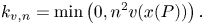
Let $n$ be a positive integer and define

Theorem 1.1 Let $R$ be a discrete valuation ring with quotient field $K$
 . Let $v$
 be the valuation of $K$
 . Let $E/K$
 be an elliptic curve defined by a Weierstrass model in minimal form with respect to $v$
 , let $P=(x,y)\in E(K)$
 and let $n$
 be a positive integer.
If $P\neq O$ is non-singular modulo $v$
 , then
If $P\neq O$ is singular modulo $v$
 , then
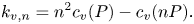
The function $c_v(nP)$ will be defined in definition 2.3 and it is periodic in $n$
 . The value of $n^2c_v(P)-c_v(nP)$
 is computed in Table 1, for the case of standard reduction types at $v$
 , and in Table 2 for the case of non-standard reduction types. The constants $m_P$
 and $a_P$
 will be defined in the next section.
Table 1. Tables of the common valuation $k_{v,n}$ for standard Kodaira types

.
Table 2. Tables of the common valuation $k_{v,n}$ for non-standard Kodaira types
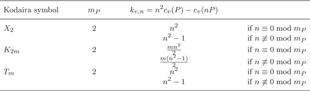
.
If the residue field $\kappa$ is perfect, then the Kodaira symbol of the curve is one of those of Table 1 and it can be computed using [Reference Silverman20, Table C.15.1]. If $\kappa$
 is not perfect, one can compute the Kodaira symbol of the curve using [Reference Szydlo22, Reference Szydlo23]. If the Kodaira symbol is not one of the symbols in Table 1 and $P$
 is singular modulo $v$
 , then the Kodaira symbol is one of those in Table 2.
We also emphasize that the formula for the cancellation $k_{v,n}$ is a quadratic polynomial in $n$
 with rational coefficients which depend only on the correction terms $c_v(P)$
 . When $K$
 is a function field of a curve over an algebraically closed field, the quantity $c_v(P)$
 was defined by other means in Cox–Zucker [Reference Cox and Zucker5] and used extensively by [Reference Shioda16] in his theory of Mordell–Weil lattices. There are two key facts that make the proof ultimately very short.
1. The Néron local height is a sum of two ingredients: local intersection pairing with the zero section and the ‘correction part’ which depends only on the component which the given point hits at the place $v$
 , cf. [Reference Lang10], [Reference Müller12],[Reference Busch and Müller2] [Reference Holmes7].
2. The valuation $v(\psi _n(P))$
is a quadratic polynomial in $n$ whose coefficients depend on the local Néron height at arguments $nP$ and $P$, respectively, and on the valuation of the minimal discriminant $\Delta$ of the elliptic curve $E$, cf. lemmas 3.3,Reference Silverman3.6. In the case of finite extensions of $\operatorname {\mathbb {Q}}_p$, this was already proven in [Reference Stange21].


On the way we reprove in our setting some results of [Reference Ayad1] and obtain a much simpler analysis of the ”troublemaker sequences’ used by Stange [Reference Stange21] and [Reference Voutier and Yabuta26] in their proofs. In the number field case, the sequence $k_{v,n}$ received considerable attention during the last 30 years, with [Reference Ayad1, Reference Cheon and Hahn3, Reference Ingram8] attempting to understand the shape of $k_{v,n}$
 . In this case, [Reference Voutier and Yabuta26] established the precise value of $k_{v,n}$
 . The goal of this paper is to extend their result to the most general setting. One can easily check that our Table 1 agrees with [Reference Voutier and Yabuta26, Table 1.1].
The study of the sequence $k_{v,n}$ has some interesting applications. For example, knowing the behaviour of $k_{v,n}$
 was necessary to show that every elliptic divisibility sequence satisfies a recurrence relation in the rational case, cf. [Reference Verzobio25]. In § 4 we will show how theorem 1.1 helps to generalize that result. Another application can be found in [Reference Stange21] and [Reference Ingram8], where the study of $k_{v,n}$
 was necessary to study the problem of understanding when a multiple of $P$
 is integral.
2. First definitions
Let $R$ be a discrete valuation ring with quotient field $K$
 and residue field $\kappa$
 . Let $v$
 be the valuation of $K$
 and assume that $v(K^*)=\operatorname {\mathbb {Z}}$
 . Let $E$
 be an elliptic curve over $K$
 which is a generic fibre of the regular proper model $\pi :\mathcal {E}\rightarrow \operatorname {Spec} R=\{o,s\}$
 . The fibre $E_s=\pi ^{-1}(s)$
 is the special fibre (singular or not). We denote by $\widetilde {\mathcal {E}}\rightarrow \operatorname {Spec} R=\{o,s\}$
 the associated Néron model which is the subscheme of smooth points over $R$
 . Assume that Weierstrass model of $E$
 is in minimal form with respect to $v$
 and let $P=(x,y)\in E(K)$
 . We denote by $\Delta$
 the discriminant of the minimal model $E$
 .
.
The point $P\in E(K)$ extends to a section $\sigma _{P}:\operatorname {Spec} R\rightarrow \overline {\mathcal {E}}$
 by the Néron model property. Let $\Phi _{v}$
 denote the group of components of the special fibre $E_s$
 . We have a natural homomorphism $comp_{v}:E(K)\rightarrow \Phi _{v}$
 which sends the point $P$
 to the element of the component group. We say that the point $P$
 is non-singular modulo $v$
 if the image $comp_v(P)$
 is the identity element, otherwise the point $P$
 is singular modulo $v$
 .
.
Let $E_0(K)\subset E(K)$ be the kernel of $comp_{v}$
 , i.e. the group of points that reduce to non-singular points modulo $v$
 . Every element $comp_{v}(P)$
 belongs to a cyclic component of $\Phi _v$
 . Let $a_P$
 be the order of this component and let $m_P$
 be the order of $comp_v(P)$
 in $\Phi _v$
 .
.
In the proof of theorem 1.1, without loss of generality, $K$ may be replaced by its completion. So, we will assume that $K$
 is complete (with respect to $v$
 ).
).
Definition 2.1 Let $(P.O)_v$ denote the local intersection number of the point $P\in E(K)\setminus \{O\}$
 with the zero point $O$
 at $v$
 defined by the formula

for the minimal model $E$ . In particular, $(P.O)_v>0$
 if and only if $P$
 reduces to the identity modulo $v$
 and then $P$
 is non-singular. For more details on local intersection, see [Reference Silverman19, Section IV.7].
Remark 2.2 For the behaviour of the sequence of integers $\{(nP.O)_v\}_n$ , see [Reference Naskręcki14, Section 7 and Lemma 8.2] in the function field case and [Reference Stange21, Lemma 5.1] in the number field case.
Definition 2.3 With a pair $(P,v)$ we associate a rational number $c_v(P)$
 which is called the correction term. Let $\widehat {\lambda _v}(P)$
 be the local Néron height as defined in [Reference Lang10, Theorem III.4.1]. Define

Remark 2.4 Observe that $c_v(P)$ depends only on $comp_v(P)$
 . This follows from [Reference Lang11, Theorem 11.5.1] when $P$
 is singular modulo $v$
 and from [Reference Silverman19, Theorem VI.4.1] when $P$
 is non-singular modulo $v$
 . In particular, [Reference Silverman19, Theorem VI.4.1] shows that $c_v(P)=0$
 when $P$
 is non-singular modulo $v$
 . In lemma 3.4 we will show how to explicitly compute $c_v(P)$
 . Finally, note that the definition of local Néron height in [Reference Lang10, Theorem III.4.1] is given for discrete valuation fields, as is noted by Lang in [Reference Lang10, p. 66].
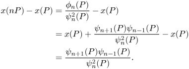
The division polynomials are defined in [Reference Silverman20, Exercise 3.7]. We recall the properties that we will use:
(A) If $nP$
is not equal to the identity $O$ of the curve, then
\[ x(nP)=\frac{\phi_n(P)}{\psi_n^2(P)}; \]
(B) The polynomials have integer coefficients and depends only on $x(P)$
. Seen as polynomials in $x(P)$, $\psi _n^2(x)$ has degree $n^2-1$ and $\phi _n(x)$ is monic and has degree $n^2$;(C) For all $n\geq 1$
,
\[ \phi_n(P)=x(P)\psi_n^2(P)-\psi_{n-1}(P)\psi_{n+1}(P). \]
(D) For all $n\geq m\geq r$
,
\[ \psi_{n+m}(P)\psi_{n-m}(P)\psi_r^2(P)=\psi_{n+r}(P)\psi_{n-r}(P)\psi_m^2(P)-\psi_{m+r}(P)\psi_{m-r}(P)\psi_n^2. \]


Remark 2.5 Our proof clearly works also for number fields. In that setting the result was known [Reference Voutier and Yabuta26], but the two proofs are completely different. Indeed, the proof of Yabuta and Voutier is almost completely arithmetical, while ours is more geometrical.
Remark 2.6 We will work assuming that $v(0)=\infty$ . Under this assumption, our theorem works also in the case when $nP=O$
 . In this case $\psi _n^2(P)=0$
 and then $k_{v,n}(P)=v(\phi _n(P))$
 .
.
3. Proof of the main theorem
We start this section by recalling some classical facts on the local Néron height.
Lemma 3.1 The following hold:
• For all $R,Q\in E(K)$
with $R,Q,R\pm Q\neq O$,
(3.1)\begin{equation} \widehat{\lambda_v}(R+Q)+\widehat{\lambda_v}(R-Q)=2\widehat{\lambda_v}(R)+2\widehat{\lambda_v}(Q)+v(x(R)-x(Q))-v(\Delta)/6. \end{equation}
• The Néron local height does not change if we replace $K$
with a finite extension. Moreover, $\widehat {\lambda _v}(\cdot )$ does not depend on the choice of the minimal Weierstrass model defining the curve.• If $comp_v(P)=comp_v(P')$
, then $\widehat {\lambda _v}(P)=\widehat {\lambda _v}(P')$.• If $P\notin E_0(K)$
, then $\widehat {\lambda _v}(P)$ just depends on the image of $P$ in $E(K)/E_0(K)$.


Proof. For the first two statements, see [Reference Lang10, Theorem III.4.1 and Page 63]. For the last two, see [Reference Lang11, Theorem 11.5.1].
Lemma 3.2 If $P$ has non-singular reduction, then

Proof. See [Reference Silverman19, Theorem VI.4.1] for the case of perfect fields and [Reference Lang10, Chapter III, §4, §5] for the general case. Observe that $\widehat {\lambda _v}(P)$ is denote by $\lambda _v(P)$
 in both [Reference Lang10, Chapter III, §4, §5] and [Reference Silverman19].
Lemma 3.3 If $nP\neq O$ , then
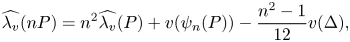
where $\Delta$ is the discriminant of the curve.
Proof. This lemma is stated as an exercise in [Reference Silverman19, Exercise 6.4 (e)]. First, assume that $P$ is a non-torsion point. We prove the lemma by induction. If $n=1$
 , it is obvious since $\psi _1(P)=1$
 . If $n=2$
 , then it follows from [Reference Silverman19, Theorem VI.1.1]. Note that, in [Reference Silverman19], it is assumed that $\kappa$
 is perfect, but the proof of the theorem works in the exact same way without that requirement, cf. [Reference Lang10, Chapter III, §4, §5]. So, we assume that the lemma is true for $i\leq n$
 and we show that it holds also for $n+1\geq 3$
 . Put $R=nP$
 and $Q=P$
 . So, $R,Q,R\pm Q\neq O$
 . Then, by lemma 3.1,

For the definition of division polynomials we have
Put $d_n=\widehat {\lambda _v}(nP)-v(\psi _{n}(P))$ and then combining (3.3) and (3.4) we have

By induction, we have $d_i=i^2d_1-(i^2-1)v(\Delta )/12$ for $i\leq n$
 and then

Therefore,

Now, we need to prove the lemma in the case when $P$ is a torsion point. Fix $n\in \mathbb {N}$
 . First, we can assume that $K$
 is complete since clearly the statement does not change. In a finite extension of $K$
 we can find a non-torsion point $P'$
 such that $(P-P'.O)_v$
 is very large. The choice of $P'$
 will depend on $n$
 . Thanks to lemma 3.1, the Néron local height does not change if we replace $K$
 with a finite extension, so we can assume $P'\in E(K)$
 . Since $(P-P'.O)_v$
 is very large, $(nP.O)_v=(nP'.O)_v$
 and $(P.O)_v=(P'.O)_v$
 (this is certainly true if $(P-P'.O)_v>(nP.O)_v$
 ). Moreover, $comp_v(P)=comp_v(P')$
 and then, from lemma 3.1, $\widehat {\lambda _v}(P)=\widehat {\lambda _v}(P')$
 and $\widehat {\lambda _v}(nP)=\widehat {\lambda _v}(nP')$
 . Furthermore, $v(\psi _n(P))=v(\psi _n(P'))$
 since $\psi _n$
 is a continuous function and $v$
 is discrete. We know that the lemma holds for $P'$
 since it is a non-torsion point and then

□
Recall that, in the case $\kappa$ perfect, the Kodaira symbol of an elliptic curve can be computed using [Reference Silverman20, Table C.15.1]. The analogous reference for the non-standard Kodaira symbols is [Reference Szydlo22, Reference Szydlo23]. Recall that $a_P$
 and $m_P$
 are defined at the beginning of § 2.
Lemma 3.4 The value of $c_v(P)$ is provided as a function of the Kodaira symbol and $m_P$
 in the following table.

In the last line, we are assuming that $0< a_P< m$ .
.
Proof. Recall that, by definition 2.3,

Assume that $P$ has non-singular reduction. By lemma 3.2, we have $\widehat {\lambda _v}(P)=v(\Delta )/12+(P.O)_v/2$
 . Hence, $c_v(P)=0$
 .
.
If $P$ has singular reduction, then $(P.O)_v=0$
 since the identity is a non-singular point. The calculation of the values of $c_v(P)$
 is based on the information obtained from the resolution of singularities performed on Weierstrass minimal model. By lemma 3.1, $\widehat {\lambda _v}(P)$
 does not depend on the choice of the minimal Weierstrass model defining the curve. So, $c_v(P)$
 does not depend on the choice of the minimal Weierstrass model.
If the residue field $\kappa$ is perfect, Tate algorithm [Reference Tate24] proves the existence of the flat proper regular model of an elliptic curve. The procedure of Tate was extended in the work of Michael Szydlo [Reference Szydlo22, Reference Szydlo23] for any elliptic curve over DVR, in particular to the case when $\kappa$
 is not a perfect field. We will refer to this general procedure as GTA (Generalized Tate's algorithm).
When $\operatorname {char}\kappa \neq 2,3$ the values of $c_v(P)$
 can be determined from the data obtained by the procedure of Tate. In fact, one follows the calculations in [Reference Cremona, Prickett and Siksek6, Proposition 6] and notes that the valuation of the minimal model and the valuation of the $(x,y)$
 coordinates of the point which reduces to the singularity are uniform across all fields with $\operatorname {char}\kappa \neq 2,3$
 , cf. [Reference Szydlo23, §4.1] and in particular [Reference Szydlo23, Table 1].
We will explain now in detail the computations for residue fields of characteristic $2$ and $3$
 , when new reduction types arise and some care must be taken. We essentially follow the strategy laid out above and supplement it with the data about valuations of the coefficients provided in [Reference Szydlo22, Reference Szydlo23]. When the fibre at $v$
 has reduction type $I_0$
 , $II$
 , $II^*$
 or any of the following non-standard Kodaira types: $Z_1, Z_2, X_1, Y_1, Y_2,Y_3, K_{2n}', K_{2n+1}$
 , the group of components is trivial (see [Reference Szydlo23, Equation (20)]).
Case $m_{P}=1$ . In such a case $P$
 has non-singular reduction and then, as we pointed out at the beginning of the proof, $c_{v}(P) = 0$
 .
.
Case $m_{P} = 2$ . Since $comp_{v}$
 is a group homomorphism and $\Phi _{v}\cong \mathbb {Z}/2\mathbb {Z}$
 it follows that if $P\not \in E_{0}(K_{v})$
 , then $c_{v}(2P) = 0$
 and $c_{v}(P) = c_{v}(3P)$
 . Moreover, $(P.O)_{v} = (3P.O)_{v} = 0$
 , hence $\widehat {\lambda _v}(P) = \widehat {\lambda _v}(3P)$
 . We get from lemma 3.3 for $n=3$
 that
that

From the definition of $c_{v}(P)$ (see equation (2.3)) we get that
For notational convenience, put $x=x(P)$ . Since $\psi _{3}(P) = 3x^4+b_2 x^3+3b_4x^2+3b_6x+b_8$
 it remains to calculate the valuation estimates for the suitable quantities. For their definition, see [Reference Silverman20, Section III.1]. By [Reference Szydlo23, Equation (20)], the only non-standard Kodaira types that we have to consider are $X_2$
 , $K_{2m}$
 , and $T_m$
 .
.
Types $III, III^*, I_{m}^*$ . We follow the argument in [Reference Cremona, Prickett and Siksek6, Proposition 6] combined with the valuation tables in [Reference Szydlo23] for the non-perfect field cases. Notice that, for these types, Tate's algorithm works in the exact same way in the perfect and non-perfect field case (see in particular [Reference Szydlo23, Tables 1, 4, 5]).
Type $X_2$ . It follows from [Reference Szydlo22, p.41] that we can construct a minimal model where $v(a_1)\geq 1$
 , $v(a_2)\geq 2$
 , $v(a_3)\geq 2$
 , $v(a_4)=2$
 , $v(a_6)\geq 4$
 and the sequence of blowups at the singular points resolve the model in such a way that the point $P=(x,y)\not \in E_0(K_v)$
 has $v(x)\geq 2$
 , cf.[Reference Szydlo23, Table 5]. It follows that $v(b_2)\geq 2$
 , $v(b_4)\geq 3$
 , $v(b_6)\geq 4$
 and finally $v(b_8) = 4$
 . Thus, we have $v(\psi _3(P))=4$
 and then $c_v(P) = 1$
 .
.
Type $K_{2m}$ . It follows from [Reference Szydlo23, Table 6] that $v(b_2)\geq 2$
 , $v(b_4)\geq 2$
 , $v(b_6)\geq 2\,m$
 , and $v(b_8) = 2\,m$
 . The resolution procedure in [Reference Szydlo22, §6.12] implies that for the minimal model with the previous assumptions we have $v(x)>m$
 . Hence, we obtain $v(\psi _{3}(P)) = 2\,m$
 , proving that $c_{v}(P) = m/2$
 .
.
Type $T_{m}$ . In the resolution [Reference Szydlo22, pp. 48-51] the valuation of $x$
 is equal to $1$
 , cf. [Reference Szydlo22, p. 51]. It follows from [Reference Szydlo23, Table 7] that all terms of $\psi _{3}(P)$
 but $3x^4$
 have valuation at least $5$
 . Hence $v(\psi _{3}(P)) = 4$
 and thus $c_v(P) = 1$
 .
.
Case $m_{P}=3$ . Type $IV, IV^*$
 . First of all, observe that $\widehat {\lambda _v}(P)=\widehat {\lambda _v}(-P)$
 . Indeed, if we put $\widehat {\lambda _v'}(P):= \widehat {\lambda _v}(-P)$
 , then $\widehat {\lambda _v'}$
 satisfies (3.1). Thanks to [Reference Lang10, Theorem III.4.1], we have $\widehat {\lambda _v'}=\widehat {\lambda _v}$
 since $\widehat {\lambda _v}$
 is unique. So, $\widehat {\lambda _v}(2P)=\widehat {\lambda _v}(-P)=\widehat {\lambda _v}(P)$
 . Using lemma 3.3 with $n=2$
 , we have

and, by (2.1),

From the definition of $\psi _2^2(P)$ we have $\psi _2^2(P)=4x(P)^3+b_2x(P)^2+2b_4x(P)+b_6$
 . Since $\widehat {\lambda _v}(P)$
 does not depend on the choice of the minimal Weierstrass equation defining the curve, we can assume that the coefficients satisfy GTA. In the case for the type $IV$
 , we have $v(b_2)>0$
 , $v(b_4)>1$
 , and $v(b_6)=2$
 . Moreover, $v(x(P))>0$
 holds due to the resolution construction. Hence,

and we are done. A very analogous calculation reveals that for the type $IV^*$ we have $c_{v}(P)=4/3$
 .
.
Case $m_{P}>3$ . We obtain for every residue field, even non-perfect the values of $c_v(P)$
 are subject to more complicated counting rule. We basically follow the argument described in [Reference Cremona, Prickett and Siksek6], enhanced by the classification of fibres by Szydlo [Reference Szydlo23].
Type $I_m^*$ $(m_P=4)$
 . Following [Reference Silverman17, p.353] we note that if $P\not \in E_{0}(K_v)$
 , then $comp_v(P)=comp_v(-3P)=comp_v(3P)$
 since $comp_v$
 is a homomorphism and $\widehat {\lambda }_{v}$
 is unique, cf. case $m_P=3$
 . Therefore, we can apply again lemma 3.3 with $n=3$
 to conclude that $c_{v}(P) = v(\psi _{3}(P))/4$
 . The explicit formulas follow from the inspections of Tables in [Reference Szydlo23].
Type $I_m$ . The correction formula for the multiplicative type can be explained in several ways. The down-to-earth approach is to invoke the theory of the Tate curve [Reference Lang10, III §5] which is independent of the residue field. We extract $c_v(P) = k(m-k)/m$
 for the intersection of $P$
 with the $k$
 -th cyclic component from [Reference Lang10, Thm. 3.5.1], cf. [Reference Silverman19, Thm. 6.4.2(b)] and [Reference Cremona, Prickett and Siksek6, Propositions 5,6].
Remark 3.5 A more conceptual approach to the proof of lemma 3.4 follows from abstract intersection theory developed by Néron, cf. [Reference Müller12]. This is an analogue of the calculations one can do in the theory of elliptic surfaces, cf. [Reference Silverman19, III §8]. This is a very general approach that would in principle allow us to calculate all correction terms using just the suitable fibral divisor. In fact, none of the references treats properly the case of non-perfect fields so we refrain from giving here all the fine details of this argument.
Lemma 3.6 Let $P$ be a point on the elliptic curve $E$
 as above. For every $n$
 such that $nP\neq O$
 , we have

In particular, $n^2 c_v(P)-c_v(nP)$ is an integer.
Proof. From (3.2) we have

From definition 2.3 we have

Hence,

□
Remark 3.7 Thanks to the previous lemma, one can easily show that the valuation $v(\psi _{n}(P))$ is independent of the choice of the minimal Weierstrass model.
Put $n_P$ as the smallest positive integer such that $n_P P$
 reduces to the identity modulo $v$
 . Observe that $n_P$
 does not necessarily exist.
Lemma 3.8 Let $k$ be an integer. If $(kP.O)_v>0$
 , then $(mkP.O)_v\geq (kP.O)_v$
 for all $m\geq 1$
 . Moreover, if $n_P$
 exists, then $(kP.O)_v>0$
 if and only if $n_P\mid k$
 .
.
Proof. Put $P':= kP$ and by assumption we have $v(x(P'))<0$
 . Hence, $v(\phi _m(P'))=m^2v(x(P'))$
 (recall that $\phi _m(P')$
 , seen as a polynomial in $x(P')$
 , is monic) and $v(\psi _m^2(P'))\geq (m^2-1)v(x(P'))$
 . So,
. So,

Now, we prove the second part of the lemma. If $n_P\mid k$ , then $(kP.O)_v>0$
 . If $n_P\nmid k$
 , then $k=qn_P+r$
 with $0< r< n_P$
 . Recall that the identity is a non-singular point of the curve reduced modulo $v$
 . Hence, if $(kP.O)_v>0$
 , then $kP$
 reduces to the identity modulo $v$
 and then also the point $rP=kP-q(n_PP)$
 reduces to the identity. This is absurd from the definition of $n_P$
 .
.
Proposition 3.9 Assume that $P$ has non-singular reduction and $(P.O)_v=0$
 . Then, $k_{v,n}(P)=0$
 for all $n\geq 1$
 .
.
Remark 3.10 This proposition was proved for number fields by Ayad [Reference Ayad1]. Their proof works also in our case, but it is very different from ours.
Proof. Since $P$ has non-singular reduction, then $c_v(kP)=0$
 for any $k$
 (see lemma 3.4). Hence, from lemma 3.6, $v(\psi _k(P)) = (kP.O)_v$
 for all $k$
 such that $kP\neq O$
 .
.
Assume $nP\neq O$ . If $(nP.O)_v>0$
 , then due to lemma 3.8 the numbers $((n-1) P.O)_v$
 and $((n+1)P.O)_v$
 are equal to zero. Therefore, $v(\psi _n(P)^2) =(nP.O)_v>0$
 , $v(\psi _{n-1}(P)\psi _{n+1}(P))=0$
 and $v(\phi _n(P)) = 0$
 from the properties (A), (B), (C), proving $k_{v,n}(P)=0$
 .
.
If $(nP.O)_v = 0$ , then $v(\psi _n(P)^2)=0$
 and $v(\phi _{n}(P))\geq 0$
 , hence again $k_{v,n}(P)=0$
 . Here we are using that the polynomials $\psi _n^2$
 and $\phi _n$
 have integer coefficients.
Assume now that $nP=O$ . Then $\psi _n^2(P)=0$
 and so $\phi _n(P)=\psi _{n-1}(P)\psi _{n+1}(P)$
 . Observe that $((n\pm 1)P.O)_v=0$
 since otherwise $(P.O)_v$
 would be strictly positive. Hence, $k_{v,n\pm 1}(P)=v(\psi _{n\pm 1}^2(P))$
 . For the first part of the lemma, $k_{v,n\pm 1}(P)=0$
 and then

□
Now, we are ready to prove our main result.
Proof Proof of theorem 1.1
Assume that $P$ has non-singular reduction. If $v(x(P))< 0$
 , then, using that $\psi _n^2$
 (resp. $\phi _n$
 ) has integer coefficients and degree $n^2-1$
 (resp. $n^2$
 ), we have $v(\psi _n^2(P))\geq (n^2-1)v(x(P))$
 and $v(\phi _n(P))=n^2v(x(P))$
 (recall that $\phi _n$
 is monic). So, $k_{v,n}(P)=n^2v(x(P))$
 . If $v(x(P))\geq 0$
 , then $(P.O)_v=0$
 and we conclude thanks to the previous proposition.
Assume now that $P$ has singular reduction, that $n_P$
 exists, and that $n_P\mid n$
 . Then, $v(x(nP))<0$
 . Therefore, $v(\phi _n(P))< v(\psi _n^2(P))$
 and so $k_{v,n}=v(\phi _n(P))$
 . Since $P$
 is singular we have $v(x(P))\geq 0$
 . Indeed, if $v(x(P))< 0$
 then $P$
 is the identity modulo $v$
 and the identity is a non-singular point. Therefore, $v(\phi _n(P))< v(x(P)\psi _n^2(P))$
 . Recall that $\phi _n(P)=x(P)\psi _n^2(P)+\psi _{n-1}(P)\psi _{n+1}(P)$
 . So,
. So,

Observe that $(n\pm 1)P\neq O$ and then in particular $((n\pm 1)P.O)_v=0$
 . Recall that $c_v(P)$
 depends only on $comp_v(P)$
 and observe that $c_v(P)=c_v(-P)$
 . Thus, $c_v((n\pm 1)P)=c_v(P)$
 since $m_P\mid n_P\mid n$
 . Hence, we can apply lemma 3.6 and we have

Thus,

Here we are using that $c_n(nP)=0$ since $nP$
 is non-singular.
It remains to prove the case when $P$ has singular reduction and that $n_P$
 does not exist or it exists but $n_P\nmid n$
 . In this case $v(x(nP))\geq 0$
 and so $k_{v,n}=v(\psi _n^2(P))\geq 0$
 . Observe that $(P.O)_v=(nP.O)_v=0$
 and then from lemma 3.6,

To conclude the proof, we want to show how to compute the values $n^2c_v(P)-c_v(nP)$ , as we did in Tables 1 and 2. If the Kodaira symbol is not $I_m$
 , then the value can be computed directly using lemma 3.4. If the Kodaira symbol is $I_m$
 , then one can easily prove that $a_{nP}\equiv a_Pn\mod m$
 . Therefore,

with $n'$ the smallest positive integer such that $a_{P}n \equiv n' \bmod {m}$
 .
.
4. A corollary and an example
In this section, we want to show an application of the main theorem and an example. Let $E$ be an elliptic curve defined by a Weierstrass equation with coefficients in the principal ideal domain $R$
 with fraction field $K$
 . Given a point $P\in E(K)$
 , one can define a sequence of integral ideals $B_n$
 that represents the square root of the denominator of the fractional ideal $(x(nP)) R$
 (the fact that the denominator is a square follows from the fact that $E$
 is defined by an equation with integer coefficients). The sequence of the $B_n$
 is a so-called elliptic divisibility sequence. If $R$
 is a principal ideal domain, we consider a choice of $\beta _n$
 such that $B_n=(\beta _n)$
 and then we have a sequence $\{\beta _n\}_{n\in \operatorname {\mathbb {N}}}$
 of elements in $R$
 such that $\beta _n$
 generates the square root of the denominator of $(x(nP))R$
 . The choice of $\beta _n$
 is clearly not unique. In [Reference Verzobio25], it is proved that, if $K=\operatorname {\mathbb {Q}}$
 and we choose the $\beta _n$
 in an appropriate way, the sequence $\{\beta _n\}_{n\in \operatorname {\mathbb {N}}}$
 satisfies a recurrence relation. The two main ingredients of the proof of this fact are the study of the behaviour of the sequence $k_{v,n}$
 for all finite places in $\operatorname {\mathbb {Q}}$
 and a recurrence relation that is satisfied by the sequence $\{\psi _n(P)\}_{n\in \operatorname {\mathbb {N}}}$
 . Thanks to the main theorem of this paper, we know the behaviour of $k_{v,n}$
 in a very general case and then we can generalize the result of [Reference Verzobio25] to the case when $K$
 is not $\operatorname {\mathbb {Q}}$
 . Indeed, we can prove the following.
Corollary 4.1 Let $R$ be a principal ideal domain with field of fractions $K$
 . Let $E$
 be an elliptic curve with a minimal Weierstrass model over $R$
 and let $P\in E(K)$
 . Define $M(P)$
 as the smallest positive integer such that $[M(P)]P$
 is non-singular modulo every maximal ideal of $R$
 .
.
We can define a sequence $\{\beta _n\}_{n\in \operatorname {\mathbb {N}}}$ of elements in $R$
 such that:
• $\beta _n$
generates the square root of the ideal generated by the denominator of $x(nP)$;• For all triples $(n,m,r)$
of positive integers such that $n\geq m\geq r$ and any two of them are multiples of $M(P)$, we have
\[ \beta_{n+m}\beta_{n-m}\beta_r^2=\beta_{n+r}\beta_{n-r}\beta_m^2-\beta_{m+r}\beta_{m-r}\beta_n^2. \]


Proof. The proof follows easily from the proof of [Reference Verzobio25, Theorem 1.9] and theorem 1.1, so we just sketch it. We define $\beta _n$ such that $\beta _n^2=\psi _n^2(P)/\gcd (\phi _n(P),\psi _n^2(P))$
 . We can define the $\gcd$
 since $R$
 is a PID. We have

We divide this equation by

and we obtain

where

Note that

If $m_1$ or $m_2$
 is a multiple of $M(P)$
 , then $v(L_{m_1,m_2})=0$
 for each $v$
 thanks to theorem 1.1. Therefore, $L_{m_1,m_2}=1$
 and, since two of $n,m,r$
 are multiples of $M(P)$
 , we have

□
Our original goal was to compute $k_{v,n}$ when $K$
 is a function field since, as we explained in the introduction, $k_{v,n}$
 is related to elliptic divisibility sequences and elliptic divisibility sequences over function fields received much attention in the last years. Hence, we show an example where we explicitly compute $k_{v,n}$
 in the function field case. For more details on the following examples, see [Reference Naskręcki13].
Example 4.2 Let $\kappa =\mathbb {C}$ , $C=\mathbb {P}_\kappa ^1$
 , and $K=\kappa (C)$
 . Then, $K=\mathbb {C}(t)$
 . Consider the elliptic curve $y^2=x(x-f^2)(x-g^2)$
 defined over $K$
 where $(f,g,h)=(t^2-1,2t,t^2+1)$
 . Notice that $f^2+g^2=h^2$
 . Let $P=((f-h)(g-h),(f+g)(f-h) (g-h)) \in E(K)$
 . We denote by $v_1$
 the place such that $v_1(t-1)=1$
 . One can easily show that $E$
 is singular modulo $v_1$
 since $v_1(f)=1$
 . Moreover $v_1(g-h)=2$
 and then $v_1(x(P))>0$
 and $v_1(y(P))>0$
 . So, $P$
 is singular modulo $v$
 . By direct computation, $v_1(\Delta _E)=4$
 and $v_1(j(E))=-4$
 . Then, $E$
 is in minimal form over $K_{v_1}$
 and $E/K_{v_1}$
 has Kodaira symbol $I_4$
 . By direct computation, $2P=(t^4 + 2t^2 + 1,-2t^5 + 2t )$
 and then $2P$
 is non-singular modulo $v_1$
 , observing that $v_1(x(2P))=0$
 . So, $a_{P,v_1} =2$
 and $m_{P,v_1}=2$
 . Using lemma 3.4, we have

Therefore, thanks to theorem 1.1,

This agrees with the direct computation of some cases for $n$ small. If $n=2$
 , then

and $v_1(\psi _2^2(P))=4$ . If $n=3$
 , then

and so $v_1(\psi _3^2(P))=8$ . Moreover, $v_1(\psi _4^2(P))=18$
 and $v_1(x(P))=2$
 . Therefore, using $\phi _n(P)=x(P)\psi _n^2(P)-\psi _{n-1}(P)\psi _{n+1}(P)$
 we obtain

and then $v(\phi _2(P))= 4$ . In the same way $v_1(\phi _3(P))= 10$
 . Hence, we conclude that $k_{v_1,2}=4$
 and $k_{v_1,3}=8$
 .
.
Acknowledgements
We want to thank Stefan Barańczuk, Matija Kazalicki, Joseph Silverman, and Paul Voutier for the comments on the earlier version of this paper. The first author acknowledges the support by Dioscuri programme initiated by the Max Planck Society, jointly managed with the National Science Centre (Poland), and mutually funded by the Polish Ministry of Science and Higher Education and the German Federal Ministry of Education and Research. The second author has been supported by MIUR (Italy) through PRIN 2017 ‘Geometric, algebraic and analytic methods in arithmetic’ and has received funding from the European Union's Horizon 2020 research and innovation programme under the Marie Skłodowska-Curie Grant Agreement No. 101034413.


 Open access