

1. Introduction
Over the last decade, the research interest in inductive power transfer (IPT) has highly increased due to a wide range of possible applications. In the daily usage of mobile phones, medical implants or electric vehicles (EVs), charging the device is an inevitable task that can benefit from IPT. The contactless charging of EVs comes with many advantages, such as user convenience, insusceptibility to weather and prevention of vandalism [Reference Zahid, Dalala and Zheng1–Reference Wang, Stielau and Covic9].
The transfer of electrical energy in inductive charging systems is proceeding via an alternating magnetic field between two coils, using the principle of resonant electromagnetic coupling via induction. This way, power can be transferred from the grid to the car through an air gap to charge the battery. Nevertheless, inductive charging results in more complex systems in comparison to conductive charging systems [Reference Niedermeier, Krammer and Schmuelling3, Reference Wu, Gilchrist and Sealy6, Reference Budhia, Covic and Boys7]. Using IPT for charging EVs, a major challenge is to design systems that work within a large area of coil positioning, due to parking inaccuracy and various ground clearances. Translatory and rotational misalignment of the coils results in a change of characteristic parameters, so it is important to be able to analyze wireless charging systems in all operating points [Reference Fotopoulou and Flynn10–Reference Sample, Meyer and Smith12]. Only if the characteristic transfer parameters of the electromagnetic coupler are known in all considered misalignments, a simulation of the system including electronic circuitry can be performed.
In this paper, we analyze the behavior of an inductive power transfer system (IPTS) when the secondary coil has a rotational offset toward the primary coil. The effect of rotational misalignment on the characteristic transfer parameters of the IPTS is evaluated and thereby a new optimal position of coils is detected. Using the three rotational angles as additional control parameters, the system can reach new operating points with high magnetic coupling and avoid operating points with low magnetic coupling.
2. Fundamentals
The block diagram in Fig. 1 shows the functional principle of an exemplary IPTS. The most elementary part for IPT is the electromagnetic coupler, which combines two resonant circuits that are galvanically isolated by the air gap. Each resonant circuit consists of an inductor and a capacitor, operating in resonance at a certain frequency f. An inverter processes the DC voltage V DC to get alternating voltage at the input side of the electromagnetic coupler, and the output voltage is rectified to charge the battery with DC voltage. As a result, alternating current resonates in the primary resonant circuit and generates an alternating magnetic field. The magnetic field induces voltage in the secondary side and thereby transfers power through an air gap by means of electromagnetic induction [Reference Zahid, Dalala and Zheng1, Reference Kim, Kong and Kim5, Reference Covic and Boys8, Reference Wang, Stielau and Covic9, Reference Mur-Miranda and Fanti13–Reference Niedermeier, Hassler, Krammer and Schmuelling15].
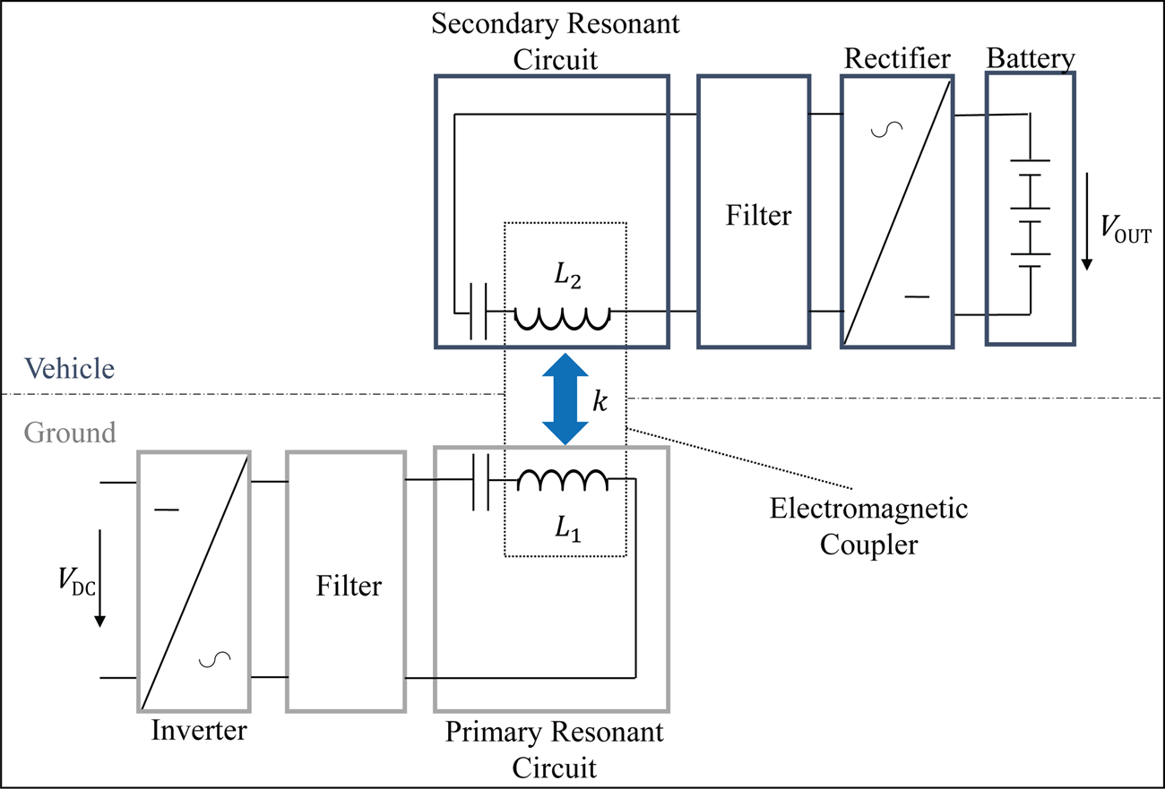
Fig. 1. Block diagram of an exemplary IPTS.
2.1. Transfer parameters
In a first approach, the electromagnetic coupler can be approximated by a transformer. The difference to a classic transformer is that the leakage inductances are much higher than the mutual inductance because there is an air gap between the coils. The established equivalent circuit of a transformer can be used to describe the electromagnetic coupler with five characteristic transfer parameters: [Reference Zahid, Dalala and Zheng1, Reference Wang, Stielau and Covic9, Reference Jiwariyavej, Imura and Hori16, Reference Schuylenbergh and Puers17]
• mutual coupling k
• primary inductance L 1
• secondary inductance L 2
• primary resistance R 1
• secondary resistance R 2
Figure 2 illustrates that the physical connectedness of the transfer parameters can be described by
 $$V_1 = j\omega L_1I_1 + R_1I_1 + j\omega MI_2$$
 $$V_2 = j\omega L_2I_2 + R_2I_2 + j\omega MI_1$$
Fig. 2. Equivalent circuit of the electromagnetic coupler.
with angular frequency ω = 2πf and mutual inductance  $M\, {=}\, k\sqrt {L_1L_2} $ [Reference Wang, Stielau and Covic9, Reference Zhang, Wong and Tse18].
The transfer parameters highly depend on the designed geometry of primary and secondary coil, on the electromagnetic properties of materials close to the coupler, and especially on the instantaneous relative position of the coils. The effect of translational misalignment has been widely investigated [Reference Niedermeier, Krammer and Schmuelling3, Reference Dang and Abu Qahouq19–Reference Liu, Yang, Jiang, Ruan and Chen22]. In this paper, we focus on the investigation of the effect of rotatory misalignment on the transfer parameters.
2.2. Optimization variable: coupling coefficient
The coupling coefficient is defined by the ratio of magnetic flux received in the secondary coil and magnetic flux generated in the primary coil. To ensure that the magnetic flux in the secondary coil is high enough to induce the defined voltage, the principle of electromagnetic resonance is used. Since the primary side is operated in resonance, a high amount of reactive power is resonating between the electric field of the capacitor and the magnetic field of the inductor. This way, the induced secondary voltage is high enough to ensure power transfer, even if the coupling coefficient is low in loosely coupled systems. However, reactive power in real systems is always accompanied by power dissipation due to cable losses and eddy current losses [Reference Abdolkhani and Coca23].
A high coupling coefficient on the other hand allows to minimize the reactive power in the system, thereby increasing the efficiency of power transfer. The development of an IPTS predominantly requires designing a coil system that offers high coupling coefficients in every allowed operating point with translational or rotatory coil offset. Thus, the coupling coefficient k is one of the most important optimization variables. This can also be seen in the equation for the optimum magnetic transformer efficiency
 $$\eta _{opt} = \displaystyle{{\chi ^2} \over {{(1 + \sqrt {1 + \chi ^2} )}^2}}\,,$$
where the figure of merit  $\chi = k\sqrt {Q_1Q_2} $ comprises the coupling coefficient with the quality factors Q 1 and Q 2 of the primary and secondary coil [Reference Vandevoorde and Puers24].
3. Method
There are two ways to get the transfer parameters of an electromagnetic coupler: measurement and simulation. In this paper, we choose simulation to be able to get the transfer parameters of the system in thousands of positions, for a more significant dataset. The following sections explain the process of modeling and simulation.
3.1. Simulation with finite element method
A number of pertinent software applications are capable of calculating the required values by means of the finite element method (FEM). For this project, ANSYS Maxwell, a high-performance software package that uses FEM to solve electromagnetic field problems, is chosen. By solving the Maxwell equations
 $$\nabla \times \vec{E} = -\displaystyle{{\partial \vec{B}} \over {\partial t}}{\rm \;\;\;\;\;\;\;\;} ;{\rm \;\;\;\;\;} \nabla \cdot \vec{D} = \rho $$
 $$\nabla \times \vec{H} = \vec{J} + \displaystyle{{\partial \vec{D}} \over {\partial t}}{\rm \;\;\;\;\;} ;{\rm \;\;\;\;\;} \nabla \cdot \vec{B} = 0$$
in a finite region with boundary conditions, ANSYS Maxwell can obtain a unique solution of electromagnetic field problems of various kinds. The finite elements are defined as tetrahedrons and the field in each element is approximated with a quadratic polynomial of second order. All values are put together to one large, sparse matrix equation that is solved by applying the Sparse Gaussian Elimination. This way, the elementary transfer parameters k, L 1, and L 2 of diverse electromagnetic couplers can be calculated via simulation with high accuracy.
3.2. Modeling
In this paper, we investigate the effect of rotation and tilt of the secondary module on the transfer parameters. Therefore, we use the circular coil system that is proposed by the Society of Automotive Engineers (SAE) in its Information Report of standard SAE J2954 [25]. The geometric modeling of the coil system can be restricted to materials that influence electromagnetic fields, so the created model only consists of aluminum, copper, and ferrite. Additional material (i.e. plastic, air, filling material) is not significant for this investigation. To reduce complexity, two simplifications are made: the ferrite tiles are modeled as one solid ferrite plate, and the windings are approximated by one solid ring with homogeneous current density. The whole model can be seen in Fig. 3, illustrating two coils, two ferrite cores and two shielding plates.

Fig. 3. Simulation model of the electromagnetic coupler.
The transfer parameters of an electromagnetic coupler highly depend on the instantaneous relative position of the coils. The SAE J2954 considers a mutual coil offset of −75 mm ≤ x ≤ 75 mm in driving direction and −100 mm ≤ y ≤ 100 mm in the transverse direction. For vertical displacement, it defines several z-classes specified by the respective ground clearances. The class z 1 is defined by a ground clearance range of 100 mm ≤ z gc ≤ 150 mm. Based on these data, the secondary coil is misaligned in x- and y-direction in the range of
 $$-{\rm 80\ mm} \le x \le {\rm 80\ mm}$$
 $$-{\rm 120\ mm} \le y \le {\rm 120\ mm}$$
with steps of 20 mm in both directions while the primary coil is fixed. The vertical distance of primary and secondary coil is set to a fixed coil-to-coil distance of z c2c = 75 mm, which corresponds roughly to the center of class z 1.
3.3. Measurements
A coil system has been built in accordance with the standard SAE J2954 to verify the simulations and the modeling method. The coil system is able to transfer up to 3.6 kW over the lateral displacement range defined in equations (6) and (7). Figure 4 shows pictures of the manufactured primary and secondary device.

Fig. 4. Photograph of the measuring object. (a) Primary coil. (b) Secondary coil.
For measuring the transfer parameters, low-power measurements are conducted. A total of 7626 positions have been measured, equally distributed over the misalignment area depicted above. The coupling coefficient of every position is compared to the respective simulated value and the results show that the simulated coupling coefficient differs from the measured coupling coefficient only by 2.65% on average. These results verify that the presented modeling method can be applied for further simulation and that the simulation results can serve as a verified base for drawing further conclusions.
3.4. Rotation and tilting of the secondary coil
Apart from translational misalignment, the coil system can also have a rotatory offset. To investigate the effect of rotatory offset, the secondary coil can be rotated in three axes: longitudinal x-axis (roll-angle: Ψ), lateral boxy-axis (pitch-angle: Θ), and vertical z-axis (yaw-angle: Φ) [25]. Figure 5 illustrates the three axes and the rotating direction. In this case, the origin of the coordinate system is set to the middle of the secondary coil, on the bottom of the copper.

Fig. 5. Three angles of rotation in relation to the secondary coil.
To get a representative dataset, the coil system is simulated for
 $$\openup 3pt\eqalign{& -6^\circ \le {\rm \;\Psi} \le 6^\circ \cr & -6^\circ \le {\rm \;\Theta} \le 6^\circ \cr & \quad\,0^\circ \le {\rm \;\Phi} \le 90^\circ} $$
with steps of 2° in Ψ and Θ, and with steps of 15° in Φ. The range of − 90° ≤ Φ < 0° is redundant due to symmetries when the secondary coil is rotating. Summing up all translational and rotatory misalignments, the coil system is simulated in 40131 different positions.
4. Results and discussion
Due to better visualization of differences that come along with rotation, the results are described as improvement potential Δk, which is defined as the percentage change of the coupling coefficient with respect to the zero-rotation value. At each allowed offset position, the secondary coil is rotated within its rotational range as stated in the previous section. First, the rotation along a single axis is studied to see the effects of each rotation direction individually. Then, the results for combinations of different rotation directions are given.
4.1. Rotation around one axis
Figure 6 shows the maximum possible improvement in the coupling coefficient that can be achieved at each position for rotation around one single axis. Figure 4 illustrates that a rotation around the x-axis can improve the coupling coefficient up to  ${\rm \Delta} k_{\rm \Psi} ^{\max} = 6.1\,\% $. The mean value taken over all positions reveals an increase in coupling coefficient of $\overline {{\rm \Delta} k_{\rm \Psi}} = 2.5\,\% $. A rotation around the y-axis yields the highest improvement for mono-axial rotation. The maximum increase is given by ${\rm \Delta} k_{\rm \Theta} ^{{\rm max}} = 8.3\,\% $ (see Fig. 4). In addition to the highest improvement, it also achieves the highest mean value with an increase of $\overline {{\rm \Delta} k_{\rm \Psi}} = 3.7\,\% $. Figure 4 shows that a single rotation around the z-axis can be neglected as it merely results in changes below 1%. The increase in coupling coefficient can be understood by consideration of the magnetic flux. The current inside the primary coil generates magnetic field lines, which have more horizontal components at a higher offset from the origin. As only the field lines perpendicular to the receiving coil induce voltage, rotation can increase the coupling coefficient. The perpendicular flux through the receiving coil can be maximized at the outer positions in particular. The magnetic field in x-direction B x increases with x-offset from the origin. Therefore, a rotation around the y-axis can increase the coupling coefficient. Analogously, at positions with y-offset the coupling coefficient can be maximized by rotating the secondary coil around the x-axis.

Fig. 6. Improvement of coupling coefficient Δk for mono-axial rotation. (a) Rotation in Ψ (around x-axis). (b) Rotation in Θ (around y-axis). (c) Rotation in Φ (around z-axis).
4.2. Rotation around two axes
The effect of rotating the receiving coil around two axes on the coupling coefficient of the system is depicted in Fig. 7. The benefits of mono-axial rotation can be combined to further exceed the improvements. Especially rotating around x- and y-axis can yield significant improvements. The highest improvement rates with  ${\rm \Delta} k_{{\rm \Psi \Theta}} ^{{\rm max}} = 13.2\,\% $ can be obtained for the outer offset positions. With an offset in x- and y-direction, the magnetic field components B x and B y raise. These components can only be utilized to raise the induced voltage when the receiving coil is tilted in both directions. The mean value over the whole offset range of Fig. 7(a) calculates to $\overline {{\rm \Delta} k_{{\rm \Psi \Theta}}} = 6.1\,\% $. A combination with z-axis rotation (see Figs 7(b) and 7(c)) severely influences the profile of the coupling coefficient x-offset for Ψ, Φ-rotation, and y-offset for Θ, Φ-rotation, but cannot support to reach higher maximum values. Table 1 gives a comprehensive overview of the maximum and mean values for the different rotation angles, including the respective inductances. Note: when considering also − 90° ≤ Φ ≤ 0° (Figs 7(b) and 7(c)) become essentially identical.

Fig. 7. Improvement of coupling coefficient Δk for bi-axial rotation. (a) Rotation in Ψ and Θ (around x, y-axes). (b) Rotation in Θ and Φ (around y, z-axes). (c) Rotation in Ψ and Φ (around x, z-axes).
Table 1. Overview of maximum change in transfer parameters.

4.3. Rotation around three axes
Figure 8 illustrates the improvement of the coupling coefficient that can be achieved for a receiving coil with a full rotational degree of freedom. Thereby, a maximum improvement of up to  ${\rm \Delta} k_{{\rm \Psi \Theta \Phi}} ^{{\rm max}} = 13.2\,\% $ can be achieved. The coupling coefficient can be increased at all positions. This is also represented in the mean value, which is raised to $\overline {{\rm \Delta} k_{{\rm \Psi \Theta \Phi}}} = 6.9\,\% $. For positions with high offset in x- and y-direction, the coupling coefficient can be raised with increasing yaw-angle until it reaches a maximum at |Φ| = 45°. Therewith, Φ-rotation can improve the coupling coefficient with up to 3%.

Fig. 8. Improvement of coupling coefficient Δk for tri-axial rotation.
4.4. Discussion
A summary of possible improvements of the coupling coefficient for different rotations in the studied offset range is given in Table 1. The highest percentage improvement can be realized when rotation around all axes is used. However, the results show that also the combined rotation around x- and y-axis is similarly potent. The study shows that the introduction of two new control parameters, roll-angle Ψ and pitch-angle Θ, can improve the coupling coefficient and therewith the system efficiency. High improvement rates of up to  $13.2\,\% $ can be achieved in particular at the outer offset positions, where low coupling coefficients prevail. In Fig. 9, the absolute coupling values are compared. Figure 9(a) shows the coupling coefficient values without rotation. In Fig. 9(b), the maximum coupling coefficient for all bi-axial rotations is depicted. It clearly shows that the absolute values are raised at all positions. In addition, it also shows that the position of the maximum values changes. Without rotation, the maximum position is at (x, y) = (0, ±60) mm while the maximum position for the system with full rotational freedom shifts to (x, y) = (0, ±80) mm. The control parameters for the new optimum are
 $${\rm \Psi} = 6^\circ {\rm \;and}$$
 $${\rm \Theta} = 0^\circ \,.$$
Fig. 9. Comparison of absolute values of coupling coefficient k. (a) Without rotation. (b) With bi-axial rotation.
Another advantage that comes with the introduction of the new control parameters Ψ and Θ is the extension of the working offset positions. The offset range is coupled to the lowest coupling coefficient, which is generally defined by maximum offset in all directions. The minimum of the coupling coefficient hence defines the possible offset range. Considering the SAE J2954 offset range and vertical coil distance z c2c = 75 mm, the minimum coupling coefficient of the system without rotation is  $k_{{\rm min}} = 19.2\,\% $ at (x, y) = ( ±75, ±100) mm. This offset range can be extended to (x, y) = ( ±90, ±120) mm with the new control parameters. The applied angles of rotation are Ψ = Θ = ±6°. This way, the allowed offset range can be increased by $44\,\% $ while maintaining the functionality and same dimensions. Alternatively, this also allows to decrease the coil size while retaining the same functional offset range.
If it is not possible to set the rotation angles as control parameters but they come as random parameters, the rotatory offset can also negatively affect k. In the worst case for the considered operating area, the coupling coefficient even decreases up to  ${\rm \Delta} k_{{\rm \Psi \Theta \Phi}} ^{wc} = -14.7\,\% $ at (x, y) = ( ±80, ±120). There, the coil is rotated by Ψ = Θ = ±6° into the opposite direction than for optimal improvement shown in the previous section. This rotation decreases the coupling coefficient, as the perpendicular flux through the receiving coil is reduced.
5. Conclusion
In this study, we use FEM simulation to evaluate the effects of rotatory coil misalignment on transfer parameters of IPTS. The results show that the coupling coefficient can be increased with each rotation axis. Highest changes in coupling coefficient can be achieved for the combination of all rotation axes. Rotation around x- and y-axis already achieves high improvements, whereas additional z-axis rotation further improves only slightly. This finding can be easily applied in EVs with air suspensions for stationary charging. The height of the air suspensions can be set individually to match the best coupling coefficient for efficient power transfer in this position. This way, two new control parameters can be utilized to extend the system performance.
 Florian Niedermeier received his B.Sc. degree in electrical engineering from the Technical University of Vienna, Austria, and his M.Sc. degree in electrical engineering from the Technical University of Munich, Germany. He is currently working on his Dr.-Ing. degree at the University of Wuppertal, Germany, and works as a research associate at BMW Group. His main research interests are simulation and analysis of inductive power transfer systems.
 Marius Hassler received his B.Sc. and M.Sc. degree in physics with specialization in condensed matter from the Technical University of Munich, Germany. He is currently working toward the Dr.-Ing. degree in engineering with BMW Group, from the Technical University of Munich, Germany. His current research interests include circuit simulation and inductive charging.
 Josef Krammer received the Dipl.-Ing. degree in electrical engineering from the Department of Electrical and Computer Engineering at the Technical University of Munich, TUM, Germany. He worked as a researcher at the Institute of Circuit Theory and Signal Processing at the TUM where he received the degree of Dr.-Ing. Since 1991 he is working at BMW Group in different engineering positions for the development of electronics for conventional and electric vehicles.
 Benedikt Schmuelling received the M.Sc. degree (Dipl.-Ing.) in electrical engineering from the Faculty of Electrical Engineering and Information Technology of Dortmund University, Germany, in 2005. From 2005 until 2010, he worked as a researcher at the Institute of Electrical Machines, RWTH Aachen University, Germany, where he also received his Ph.D. degree in 2009. From 2010 until 2012, he was with Vahle Inc., Kamen, Germany, where he worked as an engineer on the development of wireless charging stations for electric vehicles. Since 2012 he is with the University of Wuppertal, Germany, where he is the head of the Chair of Electric Mobility and Energy Storage Systems at the School of Electrical, Information and Media Engineering. His research fields include electric mobility, wireless power transfer, renewable energies, energy storage systems, and efficiency topics.


 Open access