

Introduction
Size heterogeneity is a recurrent issue in aquaculture, since it largely facilitates the exercise of cannibalism (Baras and Jobling, Reference Baras and Jobling2002; Kestemont et al., Reference Kestemont, Jourdan, Houbart, Mélard, Paspatis, Fontaine, Cuvier, Kentouri and Baras2003) and frequently imposes grading practices. Growth dispersal among cultured animals is not specific to fish, but it is generally more intense among fish than among other taxa. According to Gjedrem (Reference Gjedrem2000), the coefficient of variation for body weight typically ranges from 7% to 10% in livestock farm animals, whereas it varies between 20% and 35% in most cultured fish species. Size heterogeneity has been extensively studied and attributed to a broad series of factors, of intrinsic or extrinsic nature. In brief, individual fish are likely to exhibit genuine capacities for growth that differ slightly, e.g., because their standard metabolic rates (Cutts et al., Reference Cutts, Adams and Campbell2001; Bang et al., Reference Bang, Grønkjaer and Malte2004) or digestive abilities are different (Lemieux et al., Reference Lemieux, Blier and Dutil1999), growth dispersal can be dependent on the degree of heterozygosity (Tiira et al., Reference Tiira, Laurila, Enberg, Piironen, Aikio, Ranta and Primmer2006). These factors are likely to be buffered or amplified by between-individual variations in food intake, which have been demonstrated on several occasions to be the driving factor behind growth depensation (e.g. Jobling and Baardvik, Reference Jobling and Baardvik1994). In theory, all environmental factors that impact on food intake and growth can impact directly on growth heterogeneity (Gelineau et al., Reference Gelineau, Corraze and Boujard1998; Jourdan et al., Reference Jourdan, Fontaine, Boujard, Vandeloise, Gardeur, Anthouard and Kestemont2000; Kestemont and Baras, Reference Kestemont and Baras2001; Kestemont et al., Reference Kestemont, Jourdan, Houbart, Mélard, Paspatis, Fontaine, Cuvier, Kentouri and Baras2003). However, it is generally admitted that differential food intake and growth heterogeneity are largely governed by social hierarchies (e.g. Jobling, Reference Jobling1985; Martins, Reference Martins2005). Hierarchies do not only refer to the primacy of size differences, but also to the propensity of individual fish to be aggressive or stressed (Martins et al., Reference Martins, Schrama and Verreth2006), and to the temporal and spatial food availability. Wherever or whenever the food supply is limited and easily defensible, its access tends to be restricted or monopolized by a few fish, that grow faster than others (e.g. Huntingford et al., Reference Huntingford, Metcalfe, Thorpe, Graham and Adams1990).
Part of the uncertainty behind the mechanisms that govern growth heterogeneity in fish owes to the difficulty in measuring food intake in vivo in fish. The ballotini methodology (Carter et al., Reference Carter, Houlihan, McCarthy and Brafield1992) is accurate, but it can be deployed on a discontinuous basis only, since it requires fish capture and deep anesthesia for X-ray analysis. Food intake can vary between times of the day or between consecutive days (Kadri et al., Reference Kadri, Metcalfe, Huntingford and Thorpe1997a and Reference Kadri, Metcalfe, Huntingford and Thorpe1997b; Millot et al., Reference Millot, Bégout, Person Le-Ruyet, Breuil, Di-Poï, Fievet, Pineau and Roué2008), so it is uncertain whether the pictures obtained from X-ray analyses are representative of the actual between-fish variations of food intake over a period of time. Behavioral studies have been done to bridge this gap, since behavior can be measured continuously, e.g. with the passive integrated transponder (PIT)-tag data entry station technology (Alanärä and Brännäs, Reference Alanärä and Brännäs1993; Baras et al., Reference Baras, Malbrouck, Colignon, Etienne, Boujard, Kestemont and Mélard2000a; Coves et al., Reference Coves, Beauchaud, Attia, Dutto, Bouchut and Bégout-Anras2006). However, behavioral measures provide an indication of the access to the feeding area or food, but not of the actual food intake. Correlations between food intake and access to food can be straightforward for restricted rewards (Alanärä and Brännäs, Reference Alanärä and Brännäs1993), but less straightforward for larger rewards, when more numerous fishes can obtain food and food intake be dependent on intrinsic skills (e.g. the capacity of orientating, lunging at and handling pellets) that can hardly be quantified with these tools (Baras et al., Reference Baras, Malbrouck, Colignon, Etienne, Boujard, Kestemont and Mélard2000a).
These difficulties led several authors to test the reliability of different hypotheses about the extrinsic or intrinsic determinism of growth heterogeneity, in particular with the use of Individual-Based Models (IBM), which was pioneered by Imsland et al. (Reference Imsland, Nilsen and Folkvord1998). In this study, we have developed a hypothetico-deductive methodology, which also relied on the IBM approach but involved a mechanistic model focused on food intake. The study was carried out in three steps, using a learning sample, then a validation sample and finally examining whether different patterns of food share among fish could account for the observed heterogeneity. The biological model was the European seabass (Dicentrarchus labrax), which is one of the most intensively cultured fish species in Europe.
Material and methods
The general methodology is presented in Figure 1.

Figure 1 Hypothetico deductive approach used in this work.
Growth model
Growth was modeled using an energetic approach (Figure 2), which was based on the energetic pathway described by Bureau et al. (Reference Bureau, Kaushik and Cho2002), but where all energy losses were grouped into a single compartment. The first steps of the energetic pathway are generally expressed as NE = α × β × γ × IE where α is the apparent coefficient of digestibility, β is the ratio between Metabolizable Energy (ME) and Digestible Energy, γ is the ratio between Net Energy (NE) and ME and IE is the ingested energy. This equation can be simplified by calculating a global ‘assimilation coefficient’ (Kooijman, Reference Kooijman2000) α′ where α′ = α × β × γ. The underlying assumption was that the rate of energy loss was stable during our experiments. Actually, we had no definite proof that this was the case, but this assumption was preferred to other alternatives, essentially because rearing conditions remained stable throughout the experiment, mortality was null and fish body mass remained within the same order of magnitude. The α′ coefficient was calculated by optimization with a learning sample (see further).

Figure 2 Compartment model for energy storage and flow (for fish), using United States National Research Council nomenclature (1981). Redrawn from Bureau et al. (Reference Bureau, Kaushik and Cho2002). FE: Fecal Energy, UE: Urine Energy, ZE: Branchial Energy, HeE: Basal Metabolism, HjE: Voluntary Activity.
Net energy is distributed between a Maintenance Energy compartment (which groups the Basal Metabolism (HeE) and Voluntary Activity (HjE)) and a Retained Energy compartment (RE, also termed Recovery Energy in Bureau et al., Reference Bureau, Kaushik and Cho2002).
In this model, like in many others (Machiels and Henken, Reference Machiels and Henken1987; Conceição et al., Reference Conceição, Verreth, Verstegen and Huisman1998; Yi, Reference Yi1998), Voluntary Activity is neglected for a series of reasons. At first, seabass in this study swam almost continuously, at a rather low swimming speed, which was deemed close to their optimum swimming speed, i.e. the speed at which the energy cost per distance traveled is lowest (Videler, Reference Videler1993). At such speeds, a 10-cm seabass might presumably swim over 100 km without incurring an energy loss greater than 10% of its body energy, by reference to examples provided by Lucas and Baras (Reference Lucas and Baras2001). Furthermore, the experimental tank was small and the body length of fish did not change substantially during the study (i.e. a 100% increase in body mass corresponds to an increase of approximately 22% of the body length), so it can be reasonably assumed that swimming costs were low and homogeneous throughout the study. Hence the Maintenance can be written as Maintenance = μW λ, where μ and λ are the parameters of the allometric function, and W is the fish live body weight. Several couples of parameters that were proposed by Bureau et al. (Reference Bureau, Kaushik and Cho2002) were tested in the model and the best fitting parameterization was retained. The parameterization used for Colossoma macropomum by Van Der Meer and Van Dam (Reference Van Der Meer and Van Dam1998) (μ = 19.5 kJ/g0.8, λ = 0.8) in the Fish Growth Simulator developed by Machiels and Henken (Reference Machiels and Henken1987) fitted the model.
Retained Energy was calculated by the difference between NE and Maintenance energy. The body weight was back-calculated from the RE stock – which cumulates the flux of RE over time – by using a ratio of 0.08 g/kJ that was calculated from the data given by Bureau et al. (Reference Bureau, Kaushik and Cho2002) and Lupatsch et al. (Reference Lupatsch, Kissil and Sklan2001). This model was individualized, i.e. each fish was explicitly described with its own energy balance. In this work, the differences between individual fishes concerned the initial body weight and the individual food intake. The model was programmed with R Software.
Experiment 1 (learning data)
Experimental design
Six-month old juvenile sibling sea bass originating from a commercial fish farm (Aquanord, Gravelines, France) were raised in eight 1700-l tanks in an indoor water-recirculating system (Fontaine et al., Reference Fontaine, Terver and Georges1996). In four tanks, fish were selected in order to produce a low initial size heterogeneity (coefficient of variation of body weight (CV = s.d./mean W) of 8.4% to 9.5%), whereas in the four other tanks, fish were selected to produce a high initial size heterogeneity (CV of 28.8% to 29.5%). The initial numbers of fish in the tanks ranged from 125 to 136. Photoperiod was set at 16L : 8D. Water temperature was set at 20 ± 1.0°C. Salinity and oxygen concentrations were maintained at 30 g NaCl/l and over 5 mg O2/l respectively. The pH remained between 7 and 8.
Sea bass were acclimatized to the experimental environment for 4 weeks before the start of the 12-week experiment. The initial fish body weight in the eight groups at the end of the acclimation period was 11 ± 0.5 g.
Sea bass were fed with formulated food (Aquastart 15, 49% proteins, 13% lipids; BioMar, Nersac, France). Food was delivered by a computerized demand-feeder (Anthouard and Wolf, Reference Anthouard and Wolf1988), which recorded each activation of the trigger (to the nearest second). Food was available 24 h per day. The pellets remaining in the demand feeder were removed and weighed twice a day (0830 h and 1800 h), so as to determine the total amount of food delivered during these periods. The average amount of food per hit was calculated from the numbers of hits during these periods.
Growth was evaluated by the Specific Growth Rate: SGR = (ln(final weight) − ln(initial weight))/time (days).
Model calibration
Only one parameter of the model (α′) was calculated by optimization with these data. The optimization consisted in finding the value of α′ that minimized the Mean Squared Error between the simulated data and the observed ones. This optimization was performed with the ‘optimize’ function implemented in R Software. The daily amount of food recorded by the self-feeder was used as an input in the model.
Experiment 2
Experimental data (validation data and test of hypothesis)
At the same time as the first experiment was run, an independent group of 135 sea bass were raised over 70 days in a tank of the same recirculating system, in the same room as the eight other tanks. The initial mean weight and CV were 11.8 g and 29.0%, respectively (N = 135 fish). The experimental conditions were identical to those of the first experiment, except that all fish had been individually tagged with PIT tags (11 mm in length × 2 mm in diameter, 0.1 g; Trovan Ltd, Cologne, Germany). PIT tags were inserted into the peritoneal cavity of anesthetized fish (2-phenoxy-ethanol, 0.3 ml/l) through a 3-mm long incision on the midventral line. The incision was closed with a single stitch of non-absorbable suture filament (Baras et al., Reference Baras, Malbrouck, Houbart, Kestemont and Mélard2000b). Seven days later, all tagged fish were controlled for tag retention, healing progress and growth and the stitch was removed. Only one of the 135 tagged fish died from surgery.
Every two weeks (days 14, 28, 42, 56 and 70), all sea bass were captured, anesthetized, weighed, identified (LID-500 portable reader; Trovan Ltd) and controlled for food intake. Food intake was determined by the ‘ballotini’ method (Carter et al., Reference Carter, Houlihan, McCarthy and Brafield1992). On each day of measurement, fish were fed with ballotini-labelled food (commercial food with 2.5% ballotini glass beads, type 8.5, size: 400 to 405 μm), which are visible inside the fish’s gut when exposed to X-rays. Six hours after the light had been turned on, fish were captured, anaesthetized and X-rayed with a portable X-ray unit (TR 80/20; Todd Research Ltd, Chelmsford, UK; 80 V–20 A, 3 s of exposure on a Kodak X-OMAT-MA 24.5 × 30 cm film). Glass beads were counted and food intake was determined by reference to a calibration curve.
Simulated data
We simulated the individual growth rates of sea bass under four hypotheses of between-individual variations of food intake. In these four hypotheses, all fish differed by their initial body weights. Food intake was hypothesized as
(a) Uniform, i.e. each fish consumed the very same amount of food.
(b) Observed food intake: evaluated by the ballotini protocol. Food intake was measured five times only during the experiment, so missing data had to be interpolated, here with a linear interpolation.
(c) % body weight: i.e. all fishes consumed equivalent amounts relative to their body weights.
(d) % body weight0.66: this hypothesis takes into account the allometric decrease of the food ration relative to body weight, so the exponent is lower than 1.00. The value of 0.66 was selected after Kooijman (Reference Kooijman2000).
In order to measure the model accuracy and the relevance of each hypothesis, the observed and simulated values were compared with simple linear models Y obsi = a + b × Y simi + ei where ‘a’ was the intercept, ‘b’ the slope, ‘e’i the residual, Y obs and Y sim were observed and simulated weight. Four parameters were used to estimate the quality of the prediction (Offner and Sauvant, Reference Offner and Sauvant2004): the determination coefficient (R 2), the residual standard deviation (RSD), the slope b of the regression (compared to an expected slope of 1.00) and the mean deviation to the bisector (Y = X). The last parameter was calculated by the difference (d) between the experimental and the simulated means, as: d = a + (b − 1)·Y mean. The confidence intervals of these parameters were calculated with bootstrap method (Efron and Tibshirani, Reference Efron and Tibshirani1986).
Results
Experimental results
The growth results are summarized in Table 1. In the first experiment (learning sample) mean SGRs ranged from 1.62% to 1.94%/day and the mean final weights from 42 to 55 g. The fish of the validation experiment (with individual data) exhibited a mean SGR of 1.85%/day and a mean final weight of 43 g, with a CV of 25%. In the first experiment, the coefficient of variation of body weight remained stable for in the tanks with a high initial CV, while it increased in those with a low initial CV.
Table 1 Growth descriptor of the experiences (standard deviations are in brackets)

SGR = specific growth rate.
Model calibration/validation
The ‘assimilation coefficient’ (α′), calculated by optimization, was 0.44. The model was validated by the data of experiment 2. During this validation procedure, only the means of the data were used and the individual data were discarded. The quality of the model adjustment is illustrated in Figure 3; the validation data are correctly simulated during the process of growth. A slight deviation can be observed for the highest point, but similar deviations were observed within the calibration data.
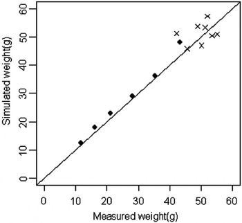
Figure 3 Model validation. The closed circles represent the calibration data. The crosses represent the validation data during the 70 days of experiment.
Hypothesis about food intake
Numerical results are presented in Table 2, and graphical results are illustrated in Figure 4. In this section only the main outcome of each simulation is given. The quality of adjustment is debated in the discussion.
Table 2 Goodness-of-fit statistics of the model under four hypotheses about individual intake

Slope = slope of the linear regression between simulated and observed body weights.
R 2 = Determination coefficient.
RSD = residual standard deviation error of the regression.
Distance = horizontal distance between the mean of the plotted points by the regression and the bisector (Y = X).
CI95% = 95% Confidence Interval, obtained by bootstrap.

Figure 4 Relationship between simulated weight and measured weight for each of the four hypotheses evaluated during this study. Each symbol (closed circle) stands for an individual fish; the bisector (i.e. observed = simulated) is symbolized by the continuous plain line while the bold dotted line is the regression model.
(a) Uniform: This simulation leads to a high R 2 coefficient (0.77), a slope that was most different from 1 (0.175) and a very low RSD (1.03).
(b) Observed food intake: The slope was very close to 1 (1.02), while the RSD was very high (13.1).
(c) % weight: The slope was close to 1.1, and the RSD was lower than 7.00 (value of 6.53)
(d) % weight0.66: The slope was less than 1 (0.61) and the RSD was low (3.6)
In every case, the distance (d) was under 7, which reflects a moderate and suitable error of the mean prediction. The relevance of each hypothesis is discussed below.
Discussion
The main objective of this study was to explore the causes of growth heterogeneity in sea bass, using an individual growth model that was specifically built for this experiment, and a hypothetico-deductive approach based on an energetic model. Imsland et al. (Reference Imsland, Nilsen and Folkvord1998) already used an Individual-Based Model to explore the causes of growth heterogeneity. In their study, six recursive growth functions were tested, which allowed calculating the individual final body weights. The base of these functions was an exponential growth model – modulated by a size effect – which was examined with three types of adjustment functions. One simulated a genetic effect by using an ‘individual stochastic growth function’ which randomly added a difference in the growth capability of each fish. The two other functions, which were termed ‘size hierarchy dependent growth rate’, were two alternative functions, which simulated – with two different formulae – the effect of the rank in the hierarchy on the growth capabilities. Their work, which was presented as the ‘first step towards a better understanding of the factors that govern size variation’, only used very synthetic functions to describe biological phenomena. Our study, which used the well-known energy balance to simulate growth, offers the possibility to investigate, with a greater accuracy, the causes of growth heterogeneity. The emphasis was laid on food intake, which is probably the most potent factor behind growth heterogeneity among fishes (Jobling and Baardvik, Reference Jobling and Baardvik1994; Martins et al., Reference Martins, Schrama and Verreth2005).
Relevance of the hypotheses
The four working hypotheses that were examined in this study as regards the way food might have been shared between fishes, gave contrasting results.
(a) Uniform: The high R 2 coefficient (0.77) indicated that simulated weight correlates with observed weight (the only source of variation of the simulated population was the heterogeneity of initial body weights). However, the slope of the relationship between simulated and observed data (0.175) indicated that the simulated heterogeneity is strongly underestimated. The low RSD was a direct consequence of the homogeneity of the simulated population. Thus, it can be concluded ab absurdo that growth heterogeneity cannot be explained by a uniform food intake among fish.
(b) Observed food intake: The slope was 1.02, but the RSD was very high (Table 2), thereby producing a wide confidence interval for the slope. Indeed, the range of the spreading width of the simulated body weights – which was calculated from the food intake data – was close to the range of the spreading width of the observed results. The simulation run under the (b) hypothesis and the method developed in Appendix suggests that the high RSD may be highly explained by the within variability of the measurement method and that the other factors would play a minor role. In order to confirm this hypothesis, the food intake should be more finely monitored in future experiments. These results are in agreement with those of Martins et al. (Reference Martins, Schrama and Verreth2005), who found that individual differences in the growth of African catfish (Clarias gariepinus) raised in isolation were mainly explained (85%) by individual differences in feed intake.
(c) % weight: The R 2 coefficient was the same as for hypothesis (a), but here the slope (1.1) was much closer to the expected value of 1.00, which indicates that growth heterogeneity was just a little overestimated. Furthermore, the RSD was low under this hypothesis, so the confidence interval for the slope is rather narrow. Altogether these descriptors suggest that this hypothesis provides a realistic picture of the actual feeding behavior of seabass, at least for the environmental conditions used in this study.
(d) % weight0.66: The RSD was low, as a direct, mathematical consequence of the flat distribution of the simulated data. On the other hand, the slope under this hypothesis was much lower than 1.00, which reveals that the growth heterogeneity of fish was strongly underestimated.
Based on these results, the most likely of the four hypotheses analyzed here is that food intake during our experiments was strictly proportional to the body weight of sea bass. This was somehow unexpected since one would have anticipated food intake relative to body weight to decrease allometrically in fish of increasing sizes, essentially because the factors that govern anabolism (gills, digestive tract, etc.) refer to surfaces, whereas catabolism is governed by body volume. This 2D : 3D ratio varies allometrically when fish grow (exponent of 0.66; Kooijman, Reference Kooijman2000), so the relationship between food intake and body weight would have been expected to follow the same dynamics in sea bass, at least among fish feeding freely. The finding that it was not the case for sea bass suggests that food intake was governed by other factors.
An exponent of 1.00 (or close to this value) indicates that the ratio between the actual and maximal food intakes of seabass was proportional to their body weight. This does not necessarily imply that the largest individuals in this study consumed more food than predicted or even that they fed maximally, but at least that they consumed more food than smaller fish did. Alternatively, it can be hypothesized that food conversion efficiency was size-dependent. There is currently no accurate information on whether food conversion varies substantially between fish of slightly different sizes, but this hypothesis is less likely than that on variable food intakes. The food supply was unlimited here, which suggests that small fishes refrained or were denied from feeding freely, and probably involves a dominance hierarchy.
There have been several studies which demonstrated that food intake was governed by dominance hierarchies, and that large, dominant fish frequently prevented smaller individuals to feed maximally and to grow at the same pace (Salmo salar, Huntingford et al., Reference Huntingford, Metcalfe, Thorpe, Graham and Adams1990; Salmo trutta, Alanärä et al., Reference Alanärä, Burns and Metcalfe2001; Perca fluviatilis, Baras et al., Reference Baras, Malbrouck, Colignon, Etienne, Boujard, Kestemont and Mélard2000a). However, these studies did not provide any model to test for this common sense hypothesis. The mathematical simulations that were evaluated here suggest that the body weight exponent in seabass is isometric (i.e. 1.00), but this might be purely contextual. Other tests should be undertaken in other rearing contexts and factors that have been demonstrated to affect growth heterogeneity, such as temperature, photoperiod, water velocity, daily food ration and stocking density (McCarthy et al., Reference McCarthy, Carter and Houlihan1992; Jobling and Baardvik, Reference Jobling and Baardvik1994; Ryer and Olla, Reference Ryer and Olla1996; Fontaine et al., Reference Fontaine, Gardeur, Kestemont and Georges1997; Stefansson et al., Reference Stefansson, FitzGerald and Cross2002).
The extent of growth heterogeneity during this experiment was partly dependent on the initial size heterogeneity. Among the groups with a high initial CV (25% to 30% body weight), size heterogeneity remained stable whereas it soared among the groups with a low initial CV (<10% body weight). These differences can be accounted for by a series of behavioral and physiological factors that govern the dynamics of dominance hierarchies. In brief, size heterogeneity frequently promotes the rapid establishment of a dominance hierarchy, generally to the detriment of the smallest individuals. However when fish are so diverse in size, their capacities for growth are most different (i.e. SGRmax is inversely proportional to body weight). In these circumstances, small fish, even if they are denied from feeding maximally, achieve growth rates that are close to those of the largest fish, so little or no further growth depensation happens. By contrast, among groups that are more homogeneous in size, the penalty for consuming less food is proportionally more severe, because the capacities for growth are more similar. Hence, growth depensation ensues, and size heterogeneity soars until an equilibrium (aforementioned situation). The ‘equilibrium’ value around which size heterogeneity eventually stabilizes is species-specific and environment-specific, since both intrinsic and extrinsic variables shape the dynamics of dominance hierarchies.
The exact reasons for why small initial differences in body weight might suffice to trigger and establish a dominance hierarchy are beyond the scope of this article. Cutts et al. (Reference Cutts, Metcalfe and Caylor1998) demonstrated that early size differences might originate from differences between the metabolic rates of individual fishes. It can also be stated that such differences might originate from different sizes at the onset of exogenous feeding, after the fish have exhausted most of their yolk reserves. Fish size at the start of exogenous feeding is largely dependent on yolk reserves, so discrepancies between egg sizes and yolk reserves might result in more or less variable feeding capacities, depending on the size of fish in respect to their prey. Whether these trends persist beyond the early feeding stages is a matter of species and environmental context, but it cannot be ruled out that some fish become dominant because they originated from larger eggs, and that others become subordinate because they survived the drawback of originating from smaller eggs. Information is currently too scant or inaccurate to validate this hypothesis, but interesting parallels can be drawn with ecological studies that referred to a ghost of predation, i.e. the anti-predator behavior being maintained even in absence of a predator (Isumbisho et al., Reference Isumbisho, Kaningini, Descy and Baras2004). In the same spirit, small sea bass might refrain from feeding maximally even if the largest fish do not represent a menace that suffices to jeopardize their survival. Simply, they are bigger, their behaviors or attitudes might be strong enough to foster this. It is clear-cut that situations where fish are raised in absence of predators are prone to stimulate this, as is typically the case of studies in monoculture. Nevertheless, even if these rules look purely artificial, they prevail nowadays among animals that are raised for feeding humans, so the importance of their understanding remains.
It is worth noticing that the learning sample in the first experiment of this study comprised both groups with high and low initial CVs, and that, in spite of this disparity, the best fit was consistently obtained with an isometric exponent in the relationship between food intake and body weight. This finding is not contradictory with the aforementioned proposed mechanism, since the value of the exponent (i.e. the slope of the log–log equation) between food intake and body weight is largely driven by the largest fish, which in these experiments corresponded to situations where the dominance hierarchy was already well established, whatever the initial size heterogeneity was high or low.
Finally, it is worth restating here that the growth rates that were simulated on the basis of measured food intakes, did not give the best fit. At first sight, this might look intriguing, since these values were measured and were assumed to illustrate as faithfully as possible the differences between individual fishes. As a matter of fact, they did to some extent, since the slope of the relationship between simulated and observed body weights was almost identical to the simulation that gave the best fit (Figure 4). However, data dispersal was much higher, and substantially reduced the quality of the fit. This is a further testimony of the limits of the ballotini technique, which is performing, but invasive, since it requires fish capture and anesthesia, so only snapshots of food intake can be obtained. These might not be representative of the actual food intake of fish over a period of time, especially if fish behavior changes between successive days or weeks (for seabass, see Millot et al., Reference Millot, Bégout, Person Le-Ruyet, Breuil, Di-Poï, Fievet, Pineau and Roué2008). Furthermore, each snapshot was taken at a particular time of the day, and it is known that feeding rhythms or food intakes vary between times of the day, depending on the status of individual fishes in the dominance hierarchy and their motivation to feed, depending, among others, on the time elapsed since the last meal (e.g. for Salmo salar, see Kadri et al., Reference Kadri, Metcalfe, Huntingford and Thorpe1997b).
In conclusion, this study provided evidence, on a mathematical basis, that food intake and growth among cultured seabass were governed by an isometric law, and this fundamentally contrasts with the knowledge on fish physiology, which unfortunately overlooks the dynamics of dominance hierarchies that are governed by behavioral registers. It further provided evidence that simulations based on actual snapshots of food intake were less reliable than mathematical simulations that were constructed on the basis of continuous dynamics, which are less subjected to subtle variations between days or meals, that strongly impact on the quality of the simulations produced with collected data. As explained above, we do not claim that food intake in cultured seabass varies isometrically with fish body weight. This was the case in this particular study, but we are aware that this might be environment-specific. Ideally, other rearing contexts should be investigated to test for this hypothesis. A particular advantage of the method that was proposed in this article, is that it enables testing a series of functional hypotheses from an hypothetico-deductive method, so datasets can be processed many times, refined and compared almost indefinitely on a consistent basis. Eventually, the use of this protocol might serve defining or predicting what are the best environmental conditions or combinations of genetic profiles that might be used to reduce size heterogeneity among cultured seabass.
Acknowledgements
The authors wish to thank the technical staff of their respective institutions for their support. This study was a follow-up of the project FAIR CT96-1572 that was funded by the European Commission (DG XIV). Special thanks to Dr Neil Wang for his fruitful scientific comments on a draft of the manuscript, and to Dominique Baras-Caseau, who improved the English style of the manuscript. Etienne Baras is an honorary research associate of the Belgian FNRS.
Appendix
It remains uncertain whether the five X-ray samples were representative of the way food was shared by fish during the experiment. Moreover, the X-ray data showed little consistency over time since the average CVi was 89% (where CVi was the coefficient of variation in the time defined as: CVi = s.d.i/meani, where s.d.i was the standard deviation of the five X-ray measurements considering the ith fish, and meani was the mean of this measurement). This observation made it necessary to evaluate the influence of this high level of noise on the simulated results. The subsequent loss of accuracy of the simulation was estimated with a Monte-Carlo method in a situation in which it was assumed that ‘growth heterogeneity resulted exclusively from by between-individual differences in food intake’ (Figure 5).

Figure 5 Monte-Carlo procedure used to evaluate modeling error caused by X-ray variability.
(i) under this assumption and according to the final and initial body weight, we calculated the theoretical proportion of food intake for each fish and considered it as constant during time.
where Ii is the individual intake of the ith fish, ΣI is the sum of every intake i.e. the total amount of food delivered and and are the initial and final body weight of the jth fish (repectively).
(ii) we calculated theoretical X-ray corresponding to the previous theoretical proportion.
(iii) we added a noise level to the theoretical X-ray. The noise was calculated with a normal law with a variance that was calculated from the observed within-individual standard deviation. Also, we could simulate a pseudo-sample of X-ray, with the same noise.
(iv) we ran 3000 simulations and compared them to the results.
With this method, we were able to observe the influence of the X-ray data noise on the final result of the simulation.
The results are shown in Table 3. The simulation run under the (b) hypotheses led to a high RSD and a low R 2. The high variability observed could be due to the within variability of recorded food intake and also to other factors that were not included in the growth model (variable activity levels and associated energy expenditures, genetic differences, etc). In order to distinguish the variability of the measure from those potential factors, we ran an additional simulation. The RSD obtained from the pseudo-noised X-ray and that from the actual X-ray (and their confidence interval) were very close. Hence the high RSD probably originated from the high within variability of the measurement method and the other factors played a minor role.
Table 3 Goodness-of-fit statistics of the model with stochastically simulated food intake

Slope = slope of the linear regression between simulated and observed body weights.
R 2 = Determination coefficient.
RSD = residual standard deviation error of the regression.
Distance = horizontal distance between the mean of the plotted points by the regression and the bisector (Y = X).
CI95% = 95% Confidence Interval, obtained by bootstrap.
a50% quantile of 3000 Monte-Carlo simulations.


 Open access